Embed Size (px)
Citation preview

13.472J/1.128J/2.158J/16.940J
COMPUTATIONAL GEOMETRY
Lecture 19
Prof. N. M. PatrikalakisCopyright c©2003 Massachusetts Institute of Technology
Contents
Decomposition models 2
19.1 Introduction . . . . . . . . . . . . . . . . . . . . . . . . . . . . . . . . . . . . . . . . . . . . 219.2 Exhaustive enumeration . . . . . . . . . . . . . . . . . . . . . . . . . . . . . . . . . . . . . 319.2.1 Definition and construction methods . . . . . . . . . . . . . . . . . . . . . . . . . . . . . 319.2.2 Applications . . . . . . . . . . . . . . . . . . . . . . . . . . . . . . . . . . . . . . . . . . 319.2.3 Properties of exhaustive enumeration methods . . . . . . . . . . . . . . . . . . . . . . . 519.3 Space subdivision . . . . . . . . . . . . . . . . . . . . . . . . . . . . . . . . . . . . . . . . . 619.3.1 Motivation and definitions . . . . . . . . . . . . . . . . . . . . . . . . . . . . . . . . . . . 619.3.2 Construction of octrees . . . . . . . . . . . . . . . . . . . . . . . . . . . . . . . . . . . . 719.3.3 Algorithms for octrees . . . . . . . . . . . . . . . . . . . . . . . . . . . . . . . . . . . . . 719.3.4 Properties of octrees . . . . . . . . . . . . . . . . . . . . . . . . . . . . . . . . . . . . . . 919.3.5 Binary space subdivision . . . . . . . . . . . . . . . . . . . . . . . . . . . . . . . . . . . 1019.4 Cell decompositions . . . . . . . . . . . . . . . . . . . . . . . . . . . . . . . . . . . . . . . 1119.4.1 Motivation . . . . . . . . . . . . . . . . . . . . . . . . . . . . . . . . . . . . . . . . . . . 1119.4.2 Cell tuple data structure . . . . . . . . . . . . . . . . . . . . . . . . . . . . . . . . . . . 1119.4.3 Properties of cell decompositions . . . . . . . . . . . . . . . . . . . . . . . . . . . . . . . 13
Integral properties of geometric models 14
19.5 Introduction . . . . . . . . . . . . . . . . . . . . . . . . . . . . . . . . . . . . . . . . . . . . 1419.6 Integral properties of curves . . . . . . . . . . . . . . . . . . . . . . . . . . . . . . . . . . . 1519.6.1 Planar curves . . . . . . . . . . . . . . . . . . . . . . . . . . . . . . . . . . . . . . . . . . 1519.6.2 3D curves . . . . . . . . . . . . . . . . . . . . . . . . . . . . . . . . . . . . . . . . . . . . 1619.7 Integral properties of surface patches . . . . . . . . . . . . . . . . . . . . . . . . . . . . . . 1719.7.1 Planar regions . . . . . . . . . . . . . . . . . . . . . . . . . . . . . . . . . . . . . . . . . 1719.7.2 Curved surface patch . . . . . . . . . . . . . . . . . . . . . . . . . . . . . . . . . . . . . 1919.8 Solids . . . . . . . . . . . . . . . . . . . . . . . . . . . . . . . . . . . . . . . . . . . . . . . 2019.9 Example: solid of revolution . . . . . . . . . . . . . . . . . . . . . . . . . . . . . . . . . . . 2219.10Appendix: Review of numerical integration methods . . . . . . . . . . . . . . . . . . . . . 2519.10.1 Trapezoidal rule of integration . . . . . . . . . . . . . . . . . . . . . . . . . . . . . . . . 2519.10.2 Simpson’s rule of integration . . . . . . . . . . . . . . . . . . . . . . . . . . . . . . . . . 2619.10.3 Romberg integration . . . . . . . . . . . . . . . . . . . . . . . . . . . . . . . . . . . . . 2719.10.4 Double integrals . . . . . . . . . . . . . . . . . . . . . . . . . . . . . . . . . . . . . . . . 28
Bibliography 31
1
Decomposition models
19.1 Introduction
Decomposition models are representations of solids via combinations (unions) of basic specialbuilding blocks glued together. Alternatively, decomposition models may be considered torepresent solids in terms of a subdivision of space (see also Lecture 1 for more details on theclassification of these models). Various types of decomposition models are created by:
• various building blocks
• various combination methods used to create the model.
In order of increasing complexity, decomposition models are classified as follows:
1. Exhaustive enumeration
2. Space subdivision
3. Cell decomposition
2
19.2 Exhaustive enumeration
19.2.1 Definition and construction methods
Exhaustive enumeration is a representation by means of nonoverlapping cubes of uniform sizeand orientation, see Figure 19.1. An object is represented by a three dimensional Boolean array.Each cell represents a cubic volume of space. If a cell intersects with the region of interest ithas a true value. Otherwise, the value is false. This can be pictured as a box divided into 3Dcubical pixels, with 0 assigned if empty and 1 assigned if full. This representation involves:
• A regular subdivision of 3D space within a cube of given size which is partitioned andoriented in a certain way within a global coordinate system. The subdivision is made upof sub-cubes (3D pixels) of given size. Reference and access to each sub-cube is made bythree integer indices i, j, k.
• For fixed space of interest we need a 3-D array, Cijk of binary data:
Cijk =
{
1 if the sub-cube i, j, k intersects the solid0 if the sub-cube i, j, k is empty
(19.1)
Construction of exhaustive enumeration models requires an alternate representation ormeasurements (eg. digital tomograghy, medical scanning, sonar data, acoustic tomographydata, etc). Usually the primary data type for such construction is a B-Rep or a CSG modelor another exhaustive enumeration model at different resolution, and cube location and orien-tation.
Operations on exhaustive enumeration models are easy. Boolean operations for example(especially for models within the same cube at the same resolution) are direct. Similarlyvisualization and integral computations are very easy. However, for higher quality rendering,filtering methods to estimate accurate surface normals may be involved [16].
The binary matrix (19.1) typically represents a valid solid. However disconnected cells orcells with low degree of connectivity as in Figure 19.2 are undesirable. For the results of Booleanoperations, filtering may be needed to maintain connectivity of cells. Strict connectivity occurswhen each full cell has at least one full neighbor across a face.
19.2.2 Applications
Applications of exhaustive enumeration methods include:
• Underwater environment representation.
• Finite element meshing (first step in an algorithm to build such a mesh).
• Medical 3D data representation.
• Preprocessing representation for speeding up operations on other representations (eg.approximating integral properties such as volume, center of gravity, moments of inertia).
3
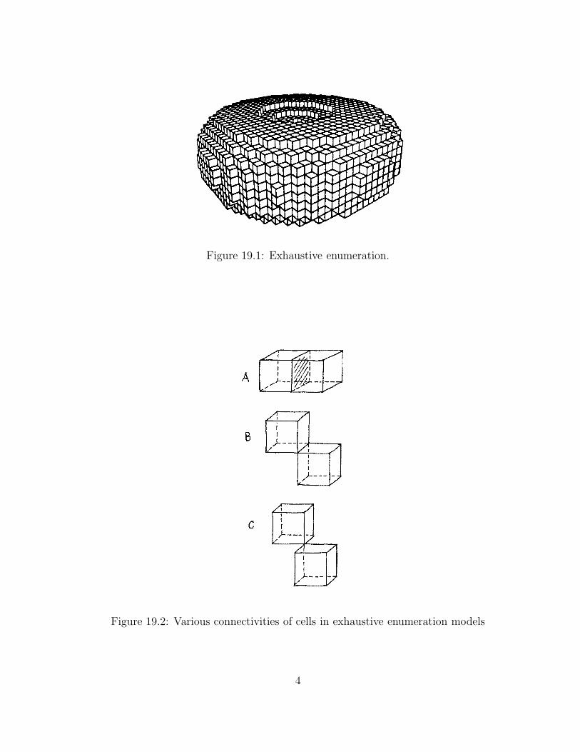
Figure 19.1: Exhaustive enumeration.
Figure 19.2: Various connectivities of cells in exhaustive enumeration models
4
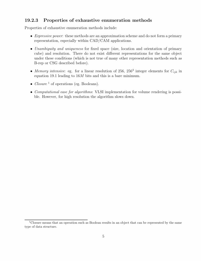
19.2.3 Properties of exhaustive enumeration methods
Properties of exhaustive enumeration methods include:
• Expressive power: these methods are an approximation scheme and do not form a primaryrepresentation, especially within CAD/CAM applications.
• Unambiguity and uniqueness for fixed space (size, location and orientation of primarycube) and resolution. There do not exist different representations for the same objectunder these conditions (which is not true of many other representation methods such asB-rep or CSG described before).
• Memory intensive: eg. for a linear resolution of 256, 2563 integer elements for Cijk inequation 19.1 leading to 16M bits and this is a bare minimum.
• Closure 1 of operations (eg. Booleans).
• Computational ease for algorithms: VLSI implementation for volume rendering is possi-ble. However, for high resolution the algorithm slows down.
1Closure means that an operation such as Boolean results in an object that can be represented by the sametype of data structure.
5
1 2
3
4
empty
1
2 3
4
full
partially full
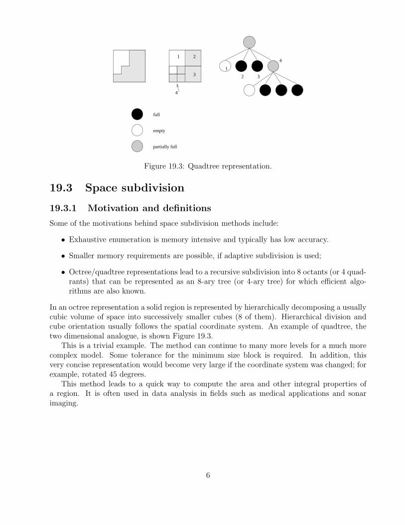
Figure 19.3: Quadtree representation.
19.3 Space subdivision
19.3.1 Motivation and definitions
Some of the motivations behind space subdivision methods include:
• Exhaustive enumeration is memory intensive and typically has low accuracy.
• Smaller memory requirements are possible, if adaptive subdivision is used;
• Octree/quadtree representations lead to a recursive subdivision into 8 octants (or 4 quad-rants) that can be represented as an 8-ary tree (or 4-ary tree) for which efficient algo-rithms are also known.
In an octree representation a solid region is represented by hierarchically decomposing a usuallycubic volume of space into successively smaller cubes (8 of them). Hierarchical division andcube orientation usually follows the spatial coordinate system. An example of quadtree, thetwo dimensional analogue, is shown Figure 19.3.
This is a trivial example. The method can continue to many more levels for a much morecomplex model. Some tolerance for the minimum size block is required. In addition, thisvery concise representation would become very large if the coordinate system was changed; forexample, rotated 45 degrees.
This method leads to a quick way to compute the area and other integral properties ofa region. It is often used in data analysis in fields such as medical applications and sonarimaging.
6
19.3.2 Construction of octrees
To create an octree, we apply a classification procedure to a given solid (represented using theBoundary Representation, Constructive Solid Geometry, or Exhaustive Enumeration methods,etc.) and decide if a given node of the octree is:
• Exterior to solid (white);
• Interior to solid (black);
• Partially interior to solid (grey).
The classification procedure is used recursively. It is based on Boolean solid operations,especially intersection. Figure 19.4 provides an simple example of octree representation.
In general, the decision if a given node of the octree is white, black, or grey is not aneasy task. For the simple case of a convex solid object, it is sufficient to classify the eightvertices of the given node of the octree (which is a cube) with respect to the solid. Thiscan be accomplished by for example casting a half-infinite ray from the point intersectingthe solid’s surfaces in a number of (multiplicity one) intersection points. If the number ofsuch intersection points is even/odd, the point is outside/in (or on the surface of the solid).However, for a concave solid object, classification of the six faces of the cube with respect tothe solid is necessary, see Figure 19.5 for an illustration in the 2-D case. This requires surfaceintersections with a planar patch. The memory and processing computation required for a 3-Dobject is on the order of the surface area of the object [12] [9]. Depending on the object andthe resolution, this can still represent a large storage requirement.
19.3.3 Algorithms for octrees
Various algorithms for octrees are developed in Meagher [12] and are summarized here:
1. Tree generation or conversion from other representation methods were discussed abovein Section 19.3.2.
2. Set operators (union, intersection, difference): A low resolution tree could be an effectivepreprocessor for a B-rep model in processes like interference checking.
3. Geometric transformations (translation, rotation, scaling).
4. Analysis procedures (integral, volume properties, connected components).
5. Rendering [16].
As an example we consider set or Boolean operations. Set operations lead to simple treetraversal
Intersection(Tree A, Tree B) = Tree CTrees are traversed in synchronous fashion and a case analysis for the types of nodes is
performed. We use the terms “black”= in-solid,“white” = out-of-solid. At each level ofsubdivision there are three cases [11]:
7
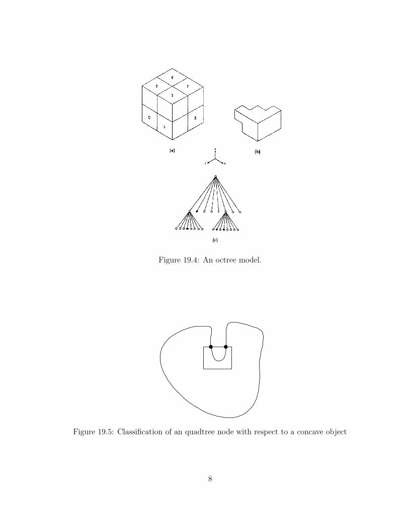
Figure 19.4: An octree model.
Figure 19.5: Classification of an quadtree node with respect to a concave object
8
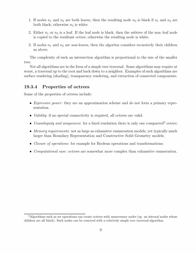
1. If nodes n1 and n2 are both leaves, then the resulting node n3 is black if n1 and n2 areboth black; otherwise n3 is white.
2. Either n1 or n2 is a leaf. If the leaf node is black, then the subtree of the non–leaf nodeis copied to the resultant octree; otherwise the resulting node is white.
3. If nodes n1 and n2 are non-leaves, then the algoritm considers recursively their childrenas above.
The complexity of such an intersection algorithm is proportional to the size of the smallertree.
Not all algorithms are in the form of a simple tree traversal. Some algorithms may require atworst, a traversal up to the root and back down to a neighbor. Examples of such algorithms aresurface rendering (shading), transparency rendering, and extraction of connected components.
19.3.4 Properties of octrees
Some of the properties of octrees include:
• Expressive power: they are an approximation scheme and do not form a primary repre-sentation.
• Validity: if no special connectivity is required, all octrees are valid.
• Unambiguity and uniqueness: for a fixed resolution there is only one compacted2 octree;
• Memory requirements: not as large as exhaustive enumeration models, yet typically muchlarger than Boundary Representation and Constructive Solid Geometry models;
• Closure of operations: for example for Boolean operations and transformations;
• Computational ease: octrees are somewhat more complex than exhaustive enumeration.
2Algorithms such as set operations can create octrees with unnecessary nodes (eg. an internal nodes whosechildren are all black). Such nodes can be removed with a relatively simple tree traversal algorithm.
9
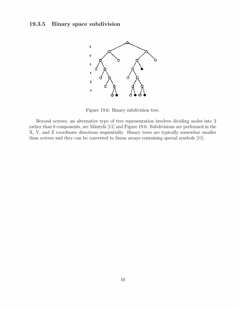
19.3.5 Binary space subdivision
Figure 19.6: Binary subdivision tree.
Beyond octrees, an alternative type of tree representation involves dividing nodes into 2rather than 8 components, see Mantyla [11] and Figure 19.6. Subdivisions are performed in theX, Y, and Z coordinate directions sequentially. Binary trees are typically somewhat smallerthan octrees and they can be converted to linear arrays containing special symbols [11].
10
19.4 Cell decompositions
19.4.1 Motivation
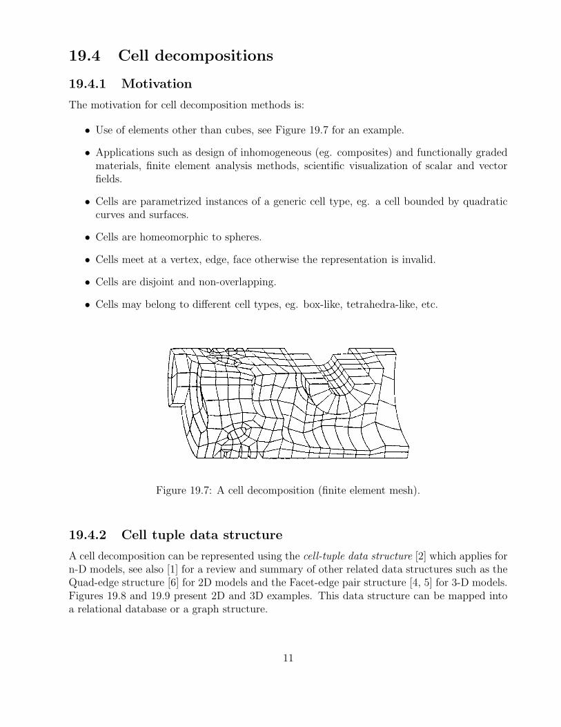
The motivation for cell decomposition methods is:
• Use of elements other than cubes, see Figure 19.7 for an example.
• Applications such as design of inhomogeneous (eg. composites) and functionally gradedmaterials, finite element analysis methods, scientific visualization of scalar and vectorfields.
• Cells are parametrized instances of a generic cell type, eg. a cell bounded by quadraticcurves and surfaces.
• Cells are homeomorphic to spheres.
• Cells meet at a vertex, edge, face otherwise the representation is invalid.
• Cells are disjoint and non-overlapping.
• Cells may belong to different cell types, eg. box-like, tetrahedra-like, etc.
Figure 19.7: A cell decomposition (finite element mesh).
19.4.2 Cell tuple data structure
A cell decomposition can be represented using the cell-tuple data structure [2] which applies forn-D models, see also [1] for a review and summary of other related data structures such as theQuad-edge structure [6] for 2D models and the Facet-edge pair structure [4, 5] for 3-D models.Figures 19.8 and 19.9 present 2D and 3D examples. This data structure can be mapped intoa relational database or a graph structure.
11
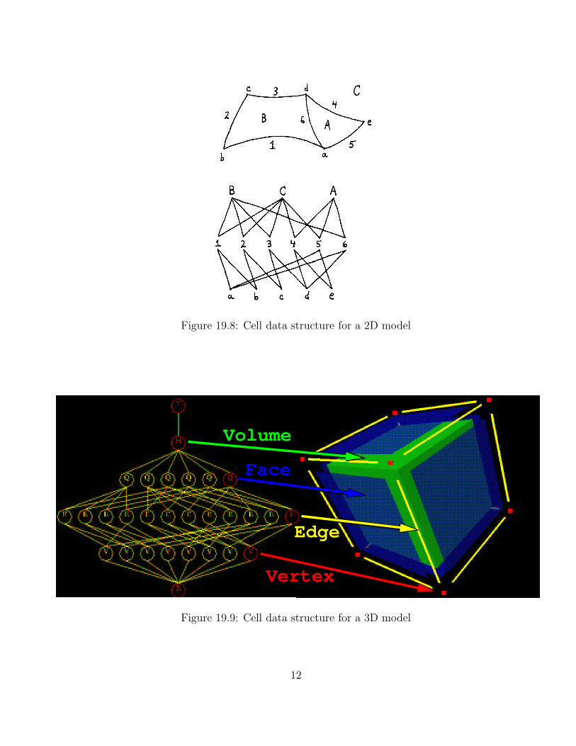
Figure 19.8: Cell data structure for a 2D model
Volume
Face
Edge
Vertex
Figure 19.9: Cell data structure for a 3D model
12

19.4.3 Properties of cell decompositions
The properties of cell decomposition methods are:
• Expressive power: they are very general and accurate, not necessarily requiring approxi-mations;
• Validity: they require an intersection test for verification;
• Unambiguity: they provide an unambiguous representation;
• Nonuniqueness: Similarly to the Constructive Solid Geometry method, the same objectcan be represented at different resolutions or with different types of mesh (eg. hexahedral,tetrahedral, etc.);
• Generation: It typically is done by conversion from other representations with or withoutgeometric approximation;
• Conciseness: memory utilization is less than octrees, yet more than Boundary Represen-tation;
• Applicability: finite element meshing, multimaterial non-homogeneous objects, visualiza-tion of fields, etc.
13
Integral properties of geometric models
19.5 Introduction
One of the important advantages of using a CAD model for representing and designing anobject is that we can easily compute the integral properties of such models such as edge curves,faces and volumes. Integral properties include length, area, centroid, moment of inertia, andvolume. These are very useful in preliminary design. For example, surface area affects drag,volume affects the carrying capacity of a vehicle, centroids are useful in hydrostatic balance,moments of inertia are used in dynamics and in hydrostatic stability calculation (for ships).
Computation of the integral properties of curves, surface patches and solids involves eval-uation of single, double and triple integrals of the form
φcurve =∫
curvef(P)dL, φsurface =
∫
surfacef(P)dS, φsolid =
∫
solidf(P)dV (19.2)
where φ is the required property, P is a point and f is a real-valued function, which depends onthe type of property required. We have studied three classes of solid representation methods inthe previous chapters, namely Decomposition methods, Constructive Solid Geometry (CSG)methods, and Boundary Representation (B-rep) methods.
For decomposition methods, the integral over the solid reduces to a sum of integrals
∫
solidfdV =
∑
i
∫
celli
fdV (19.3)
where celli is the i − th cell which is either full or partially full. For the case of exhaustivespatial enumeration the cells are constant-sized cubes and for the octree decompositions theyare variable-sized cubes [10, 13]. For high resolution models it is enough to consider all thecelli to be full entirely and for those cases the resulting integrals are elementary and can becomputed using simple analytic forms.
As we have studied in the previous chapters, CSG is a tree whose nodes represent theBoolean operators and the leaves are the primitive solids. Therefore the computation of integralproperties of CSG solids consists of applying the following formula recursively [10]:
∫
A∪BfdV =
∫
AfdV +
∫
BfdV −
∫
A∩BfdV (19.4)
∫
A−BfdV =
∫
AfdV −
∫
A∩BfdV. (19.5)
14

Consequently we need to compute integrals over primitives (which can be evaluated analyti-cally) and integrals involving intersections of primitives
∫
A∩B fdV which can be approximatedusing a ray casting, ray classification and integral approximation method.
Boundary representation, which is the most generally used representation today, representsthe object in terms of their boundary elements (e.g. vertices, edges, faces). For evaluating theintegral properties for B-rep solids, the following theorems from vector calculus are useful [7]:
1. Green’s TheoremIf C is a piecewise smooth, simple closed curve that bounds a region R, and if P (x, y)and Q(x, y) are continuous functions which have continuous partial derivatives along C
and throughout R, then
∮
C(Pdx + Qdy) =
∫∫
R
(
∂Q
∂x− ∂P
∂y
)
dA (19.6)
2. Divergence Theorem (also called Gauss’ Theorem)The flux of vector field F flowing outward through a closed surface S equals the integralof the divergence of F over the region R bounded by S;
∫∫
SF · ndA =
∫∫∫
R∇FdV (19.7)
where n is the outward unit normal vector and
∇ · F =∂F
∂x· i +
∂F
∂y· j +
∂F
∂z· k. (19.8)
where i, j, k are the unit coordinate vectors.
In the sequel we will apply these theorems to compute the integral properties of geometricmodels represented by the B-rep method (in 1-3 dimensions).
19.6 Integral properties of curves
19.6.1 Planar curves
Let a planar curve be defined by
r = (x(t), y(t)) , to ≤ t ≤ t1 (19.9)
• Length
L =∫ s1
s0
ds =∫ t1
t0
√
r(t) · r(t)dt (19.10)
=∫ t1
t0
√
x2(t) + y2(t)dt
15
• “Centroid”
rc = (xc, yc) =
∫ s1
s0rds
∫ s1
s0ds
(19.11)
=1
L
∫ t1
t0
r(t)√
x2(t) + y2(t)dt
• “Moments of inertia”
Ixx =∫ s1
s0
y2ds =∫ t1
t0
y2(t)√
x2(t) + y2(t)dt (19.12)
Iyy =∫ s1
s0
x2ds =∫ t1
t0
x2(t)√
x2(t) + y2(t)dt (19.13)
Ixy =∫ s1
s0
xyds =∫ t1
t0
x(t)y(t)√
x2(t) + y2(t)dt (19.14)
19.6.2 3D curves
Let a 3D curve be defined by
r = (x(t), y(t), z(t)) , to ≤ t ≤ t1 (19.15)
• Length
L =∫ s1
s0
ds =∫ t1
t0
√
r(t) · r(t)dt (19.16)
=∫ t1
t0
√
x2(t) + y2(t) + z2(t)dt
• “Centroid”
rc = (xc, yc, zc) =
∫ s1
s0rds
∫ s1
s0ds
(19.17)
=1
L
∫ t1
t0
r(t)√
x2(t) + y2(t) + z2(t)dt
• “Moments of inertia”
Ixx =∫ s1
s0
(y2 + z2)ds =∫ t1
t0
(
y2(t) + z2(t))
√
x2(t) + y2(t) + z2(t)dt (19.18)
Iyy =∫ s1
s0
(x2 + z2)ds =∫ t1
t0
(
x2(t) + z2(t))√
x2(t) + y2(t) + z2(t)dt (19.19)
Izz =∫ s1
s0
(x2 + y2)ds =∫ t1
t0
(
x2(t) + y2(t))
√
x2(t) + y2(t) + z2(t)dt (19.20)
Ixy =∫ s1
s0
xyds =∫ t1
t0
x(t)y(t)√
x2(t) + y2(t) + z2(t)dt (19.21)
Iyz =∫ s1
s0
yzds =∫ t1
t0
y(t)z(t)√
x2(t) + y2(t) + z2(t)dt (19.22)
Ixz =∫ s1
s0
xzds =∫ t1
t0
x(t)z(t)√
x2(t) + y2(t) + z2(t)dt (19.23)
16
19.7 Integral properties of surface patches
19.7.1 Planar regions
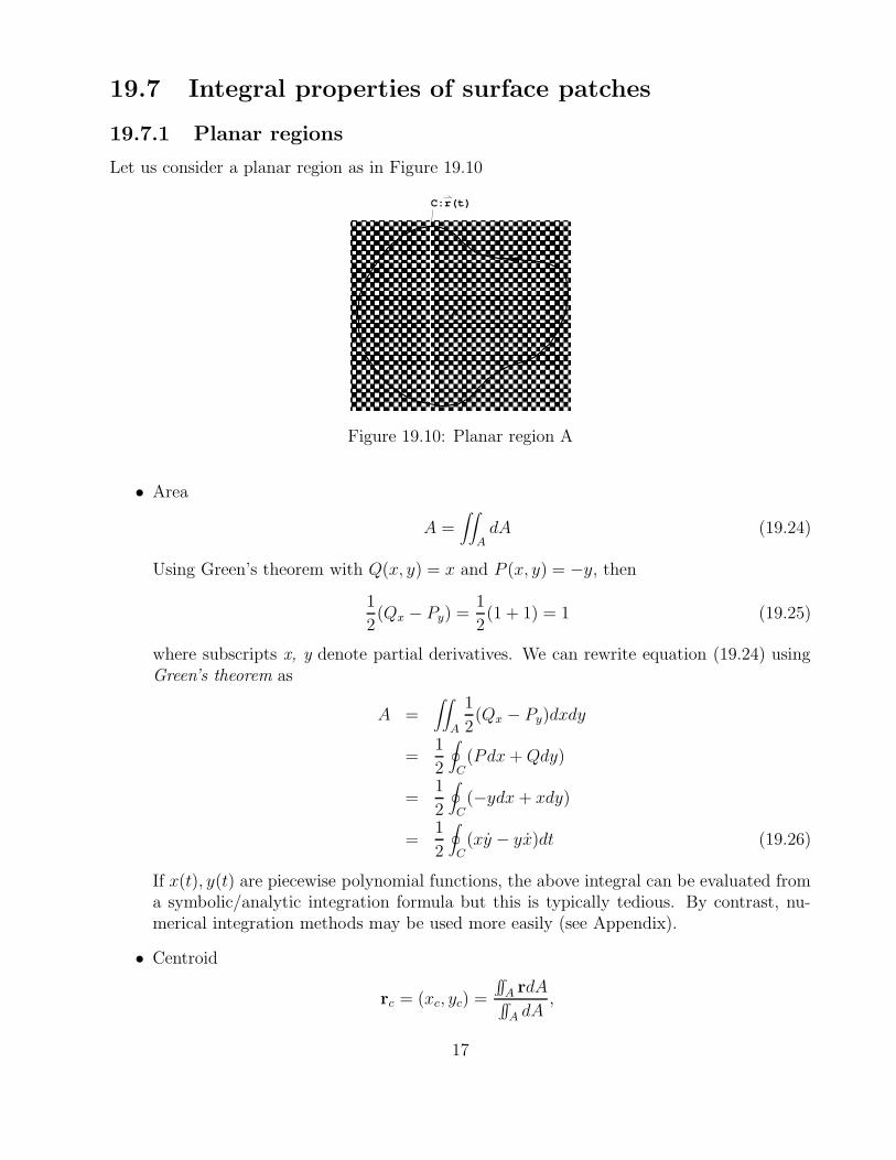
Let us consider a planar region as in Figure 19.10
�������������������������������������������������������������������������������������������������������������������������������������������������������������������������������������������������������������������������������������������������������������������������������������������������������������������������������������������������������������������������������������������������������������������������������������������������������������������������������������������������������������������������������������������������������������������������������������������������������������������������������������������������������������������������������������������������������������������������������������������������������������������������������������������������������������������������������������������������
C:r(t)
A
Figure 19.10: Planar region A
• Area
A =∫∫
AdA (19.24)
Using Green’s theorem with Q(x, y) = x and P (x, y) = −y, then
1
2(Qx − Py) =
1
2(1 + 1) = 1 (19.25)
where subscripts x, y denote partial derivatives. We can rewrite equation (19.24) usingGreen’s theorem as
A =∫∫
A
1
2(Qx − Py)dxdy
=1
2
∮
C(Pdx + Qdy)
=1
2
∮
C(−ydx + xdy)
=1
2
∮
C(xy − yx)dt (19.26)
If x(t), y(t) are piecewise polynomial functions, the above integral can be evaluated froma symbolic/analytic integration formula but this is typically tedious. By contrast, nu-merical integration methods may be used more easily (see Appendix).
• Centroid
rc = (xc, yc) =
∫∫
A rdA∫∫
A dA,
17
where A is the shaded area, and
∫∫
ArdA =
(∫∫
AxdA,
∫∫
AydA
)
. (19.27)
Let Q(x, y) = x2
2, P (x, y) = 0, then
Qx − Py = x − 0 = x (19.28)
Therefore∫∫
AxdA =
∮
CPdx + Qdy =
∮
Cx2dy (19.29)
where C is the complete boundary of A. Thus,
xc =
∫∫
A xdA∫∫
A dA
=1
A
∫∫
AxdA
=1
A
∮
Cx2ydt (19.30)
Let Q(x, y) = 0, P (x, y) = − y2
2, then
Qx − Py = 0 + y = y (19.31)
Similarly,
yc =
∫∫
A ydA∫∫
A dA
=1
A
∫∫
AydA
= − 1
A
∮
Cy2xdt (19.32)
• Moments of inertia
1. Ixx =∫∫
A y2dA
Let Q(x, y) = 0, P (x, y) = − y3
3, then
Qx − Py = y2 (19.33)
Using Green’s Theorem,
Ixx =∫∫
A(Qx − Py)dxdy =
∮
C−y3dx
= −∮
Cy3xdt (19.34)
18
2. Iyy =∫∫
A x2dA
Let Q(x, y) = x3
3, P (x, y) = 0, then
Qx − Py = x2 (19.35)
Using Green’s Theorem,
Iyy =∫∫
A(Qx − Py)dxdy =
1
4
∮
C
x3
3dy
=∮
Cx3ydt (19.36)
3. Ixy =∫∫
A xydA
Let Q(x, y) = x2y
2, P (x, y) = 0, then
Qx − Py = xy + 0 = xy (19.37)
Using Green’s Theorem,
Ixy =∫∫
A(Qx − Py)dxdy
=1
2
∮
Cx2yydt (19.38)
If x(t), y(t) are piecewise polynomial functions, the above integrals can be evaluatedfrom a symbolic/analytic integration formula but this is typically tedious. By contrast,numerical integration methods may be used more easily (see Appendix).
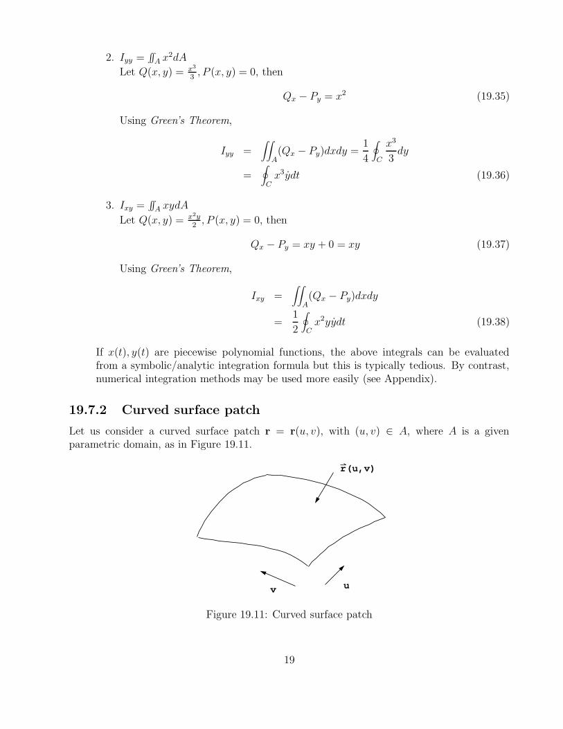
19.7.2 Curved surface patch
Let us consider a curved surface patch r = r(u, v), with (u, v) ∈ A, where A is a givenparametric domain, as in Figure 19.11.
r(u,v)
v u
Figure 19.11: Curved surface patch
19
• Area
A =∫∫
AdA
=∫∫
A|ru × rv|dudv =
∫∫
A
√EG − F 2dudv (19.39)
where E, F and G are the first fundamental form coefficients E = ru·ru, F = ru·rv, G =rv · rv. (see Chapter 2).
• “Centroid”
rc = (xc, yc, zc) =
∫∫
A rdA∫∫
A dA
=1
A
∫∫
A[x(u, v), y(u, v), z(u, v)]
√EG − F 2dudv (19.40)
• “Moments of inertia”
Ixx =∫∫
A[y2(u, v) + z2(u, v)]
√EG − F 2dudv (19.41)
Iyy =∫∫
A[x2(u, v) + z2(u, v)]
√EG − F 2dudv (19.42)
Izz =∫∫
A[x2(u, v) + y2(u, v)]
√EG − F 2dudv (19.43)
Ixy =∫∫
A[x(u, v)y(u, v)]
√EG − F 2dudv (19.44)
Ixz =∫∫
A[x(u, v)z(u, v)]
√EG − F 2dudv (19.45)
Iyz =∫∫
A[y(u, v)z(u, v)]
√EG − F 2dudv (19.46)
Integrals 19.39-19.46 may be evaluated numerically as in the Appendix.
19.8 Solids
For solids described by the B-rep method it is convenient to transform volume integrals intosurface integrals by means of the divergence theorem.
• Volume
V =∫∫∫
VdV (19.47)
Choose
r = xi + yj + zk (19.48)
then
∇ · r =∂r
∂x· i +
∂r
∂y· j +
∂r
∂z· k = 3 (19.49)
20
Using the Divergence (or Gauss’) Theorem,
V =∫∫∫
VdV =
1
3
∫∫∫
V∇ · rdV
=1
3
∫∫
Ar · ndA =
1
3
∫∫
Ar · n|ru × rv|dudv
=1
3
∫∫
Ar · (ru × rv)dudv (19.50)
given that
n =ru × rv
|ru × rv|(19.51)
• Centroid
rc = (xc, yc, zc) =
∫∫∫
V rdV∫∫∫
V dV(19.52)
Choose
r =1
2x2i (19.53)
then
∇ · r =∂r
∂x· i +
∂r
∂y· j +
∂r
∂z· k = x (19.54)
xc =1
V
∫∫∫
VxdV =
1
V
∫∫∫
V∇ · rdV
=1
V
∫∫
A
1
2x2(i · n)dA
=1
V
∫∫
A
1
2x2(i · (ru × rv))dudv (19.55)
Similarly, expressions are obtained for yc, zc:
yc =1
V
∫∫
A
1
2y2(j · (ru × rv))dudv (19.56)
zc =1
V
∫∫
A
1
2z2(k · (ru × rv))dudv (19.57)
• Moments of inertia
Ixx =∫∫∫
V(y2 + z2)dV (19.58)
Choose
r = (y2 + z2)xi (19.59)
21
then
∇ · r =∂r
∂x· i +
∂r
∂y· j +
∂r
∂z· k = y2 + z2 (19.60)
Thus
Ixx =∫∫∫
V(y2 + z2)dV =
∫∫∫
V∇ · rdV
=∫∫
A(y2 + z2)x(i · n)dA
=∫∫
A(y2 + z2)x(i · (ru × rv))dudv (19.61)
Similarly,
Iyy =∫∫
A(x2 + z2)y(j · (ru × rv))dudv (19.62)
Izz =∫∫
A(x2 + y2)z(k · (ru × rv))dudv (19.63)
Ixy =∫∫
Axyz(k · (ru × rv))dudv (19.64)
Ixz =∫∫
Axzy(j · (ru × rv))dudv (19.65)
Iyz =∫∫
Ayzx(i · (ru × rv))dudv (19.66)
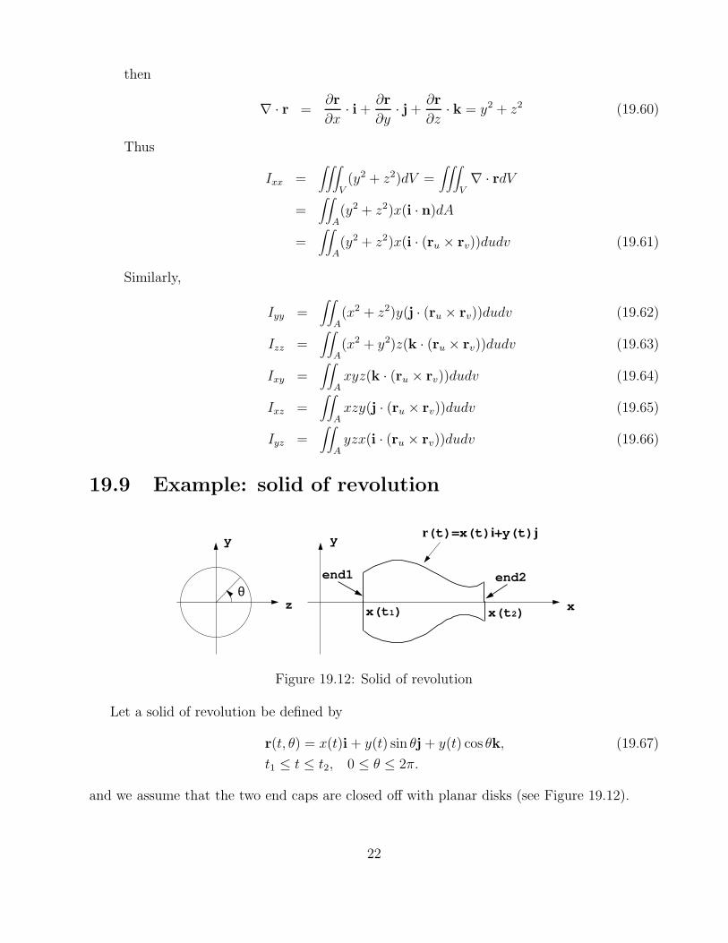
19.9 Example: solid of revolution
r(t)=x(t)i+y(t)j
x
yy
zθ
end1 end2
x(t1) x(t2)
Figure 19.12: Solid of revolution
Let a solid of revolution be defined by
r(t, θ) = x(t)i + y(t) sin θj + y(t) cos θk, (19.67)
t1 ≤ t ≤ t2, 0 ≤ θ ≤ 2π.
and we assume that the two end caps are closed off with planar disks (see Figure 19.12).
22
• Surface area of surface of revolution (with end caps)
rt = (x, y sin θ, y cos θ) (19.68)
rθ = (0, y cos θ,−y sin θ) (19.69)
rt × rθ =
∣
∣
∣
∣
∣
∣
∣
i j kx y sin θ y cos θ
0 y cos θ −y sin θ
∣
∣
∣
∣
∣
∣
∣
= (−yy sin2 θ − yy cos2 θ)i + xy sin θj + xy cos θk
= −yyi + xy sin θj + xy cos θk (19.70)
|rt × rθ| =√
y2y2 + x2y2 = y√
x2 + y2 (19.71)
A =∫∫
AdA =
∫ t2
t1
∫ 2π
0y√
x2 + y2dθdt
= 2π∫ t2
t1
y√
x2 + y2dt (19.72)
• Volume
rt × rθ = (−yy, xy sin θ, xy cos θ) (19.73)
r · (rt × rθ) = (x, y sin θ, y cos θ) · (−yy, xy sin θ, xy cos θ)
= −xyy + xy2 sin2 θ + xy2 cos2 θ
= −xyy + xy2 (19.74)
V =1
3
∫ t2
t1
∫ 2π
0r · (rt × rθ)dtdθ − 1
3
∫∫
Aend1
xdxdy +1
3
∫∫
Aend2
xdxdy
=1
3
∫ t2
t1
∫ 2π
0(−xyy + xy2)dθdt − π
3x(t1)y
2(t1) +π
3x(t2)y
2(t2)
=2π
3
∫ t2
t1
(−xyy + xy2)dt − π
3x(t1)y
2(t1) +π
3x(t2)y
2(t2) (19.75)
Using integration by parts,
−∫ t2
t1
xyydt = −[xy2]t2t1 +∫ t2
t1
(xy)′ydt
= −x(t2)y2(t2) + x(t1)y
2(t1) +∫ t2
t1
(xy2 + xyy)dt (19.76)
Thus
−2∫ t2
t1
xyydt = −x(t2)y2(t2) + x(t1)y
2(t1) +∫ t2
t1
xy2dt (19.77)
23
The volume, therefore, is
V =2π
3
∫ t2
t1
xy2dt − 2π
3
∫ t2
t1
(−xyy)dt − π
3x(t1)y
2(t1) +π
3x(t2)y
2(t2)
= π
∫ t2
t1
xy2dt (19.78)
(corroborating the obvious formula from elementary calculus)
• Centroid
1. i · (rt × rθ) = −yy
xc =1
V
∫ t2
t1
∫ 2π
0
1
2x2(−yy)dtdθ − π
2Vx2(t1)y
2(t1) +π
2Vx2(t2)y
2(t2)
=π
V
∫ t2
t1
(−x2yy)dt +π
2V(x2(t2)y
2(t2) − x2(t1)y2(t1)) (19.79)
Integrate by parts
−∫ t2
t1
x2yydt = −[x2y2]t2t1 +∫ t2
t1
(x2y)′ydt
= −x2(t2)y2(t2) + x2(t1)y
2(t1) +∫ t2
t1
(2xxy + x2y)ydt (19.80)
Thus
−2∫ t2
t1
x2yydt = −x2(t2)y2(t2) + x2(t1)y
2(t1) + 2∫ t2
t1
xxy2dt (19.81)
and
xc =π
V
∫ t2
t1
xxy2dt (19.82)
(corroborating the obvious formula from elementary calculus)
2. j · (rt × rθ) = xy sin θ
yc =1
V
∫∫
A
1
2y2xy sin θdtdθ
=1
2V
∫ t2
t1
∫ 2π
0y3x sin θdθdt
=1
2V
∫ t2
t1
y3x[− cos θ]2π0 dt
= 0 (19.83)
3. k · (rt × rθ) = xy cos θ
zc =1
V
∫∫
A
1
2z2xy cos θdtdθ
=1
2V
∫ t2
t1
∫ 2π
0xyz2 cos θdθdt
=1
2V
∫ t2
t1
xyz2[sin θ]2π0 dt
= 0 (19.84)
24
19.10 Appendix: Review of numerical integration meth-
ods
19.10.1 Trapezoidal rule of integration
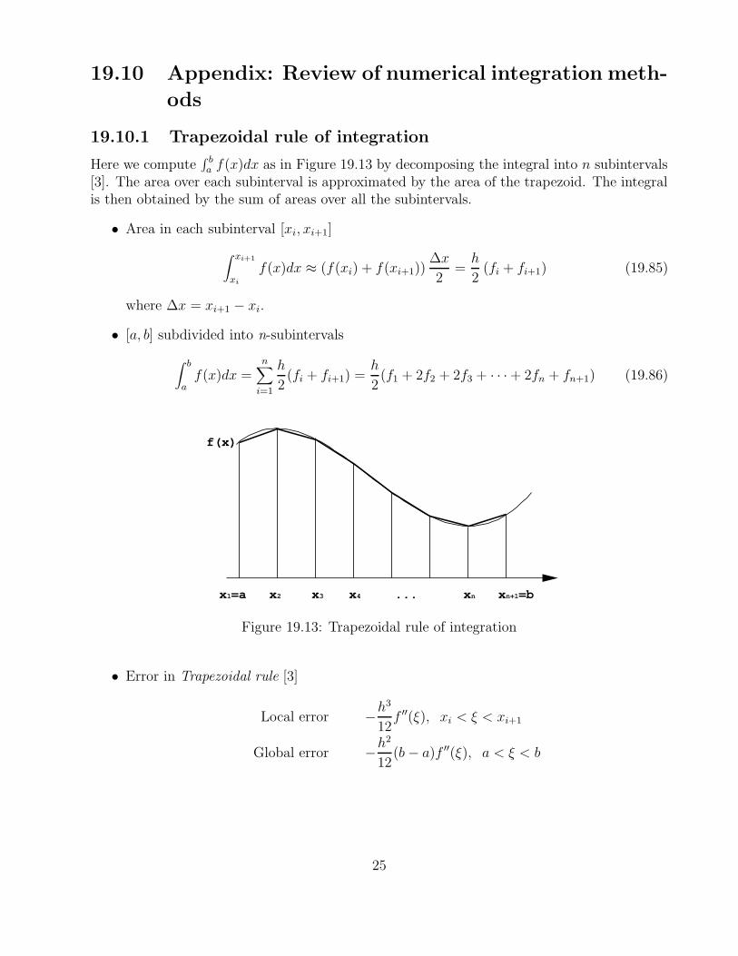
Here we compute∫ ba f(x)dx as in Figure 19.13 by decomposing the integral into n subintervals
[3]. The area over each subinterval is approximated by the area of the trapezoid. The integralis then obtained by the sum of areas over all the subintervals.
• Area in each subinterval [xi, xi+1]
∫ xi+1
xi
f(x)dx ≈ (f(xi) + f(xi+1))∆x
2=
h
2(fi + fi+1) (19.85)
where ∆x = xi+1 − xi.
• [a, b] subdivided into n-subintervals
∫ b
af(x)dx =
n∑
i=1
h
2(fi + fi+1) =
h
2(f1 + 2f2 + 2f3 + · · ·+ 2fn + fn+1) (19.86)
x1=a x2 x3 x4 ... xn xn+1=b
f(x)
Figure 19.13: Trapezoidal rule of integration
• Error in Trapezoidal rule [3]
Local error −h3
12f ′′(ξ), xi < ξ < xi+1
Global error −h2
12(b − a)f ′′(ξ), a < ξ < b
25
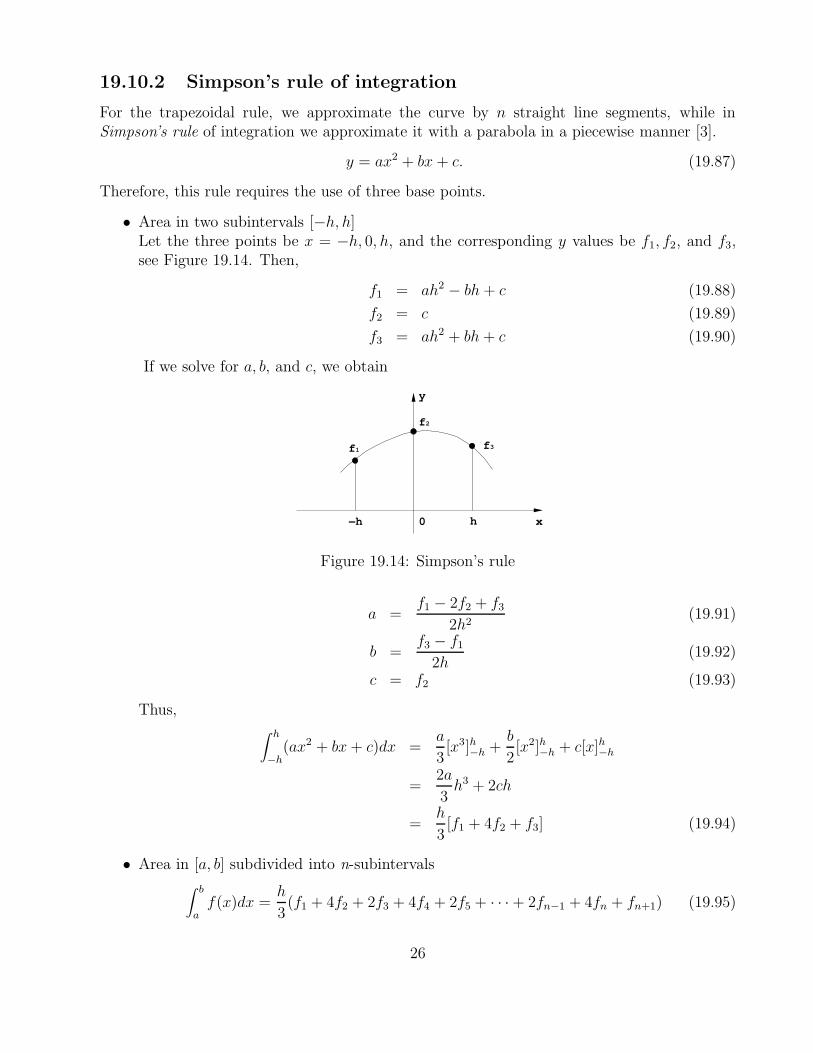
19.10.2 Simpson’s rule of integration
For the trapezoidal rule, we approximate the curve by n straight line segments, while inSimpson’s rule of integration we approximate it with a parabola in a piecewise manner [3].
y = ax2 + bx + c. (19.87)
Therefore, this rule requires the use of three base points.
• Area in two subintervals [−h, h]Let the three points be x = −h, 0, h, and the corresponding y values be f1, f2, and f3,see Figure 19.14. Then,
f1 = ah2 − bh + c (19.88)
f2 = c (19.89)
f3 = ah2 + bh + c (19.90)
If we solve for a, b, and c, we obtain
−h 0 x
y
f 2
f 1 f 3
h
Figure 19.14: Simpson’s rule
a =f1 − 2f2 + f3
2h2(19.91)
b =f3 − f1
2h(19.92)
c = f2 (19.93)
Thus,∫ h
−h(ax2 + bx + c)dx =
a
3[x3]h
−h +b
2[x2]h
−h + c[x]h−h
=2a
3h3 + 2ch
=h
3[f1 + 4f2 + f3] (19.94)
• Area in [a, b] subdivided into n-subintervals∫ b
af(x)dx =
h
3(f1 + 4f2 + 2f3 + 4f4 + 2f5 + · · · + 2fn−1 + 4fn + fn+1) (19.95)
26
• Error in Simpson’s rule [3]
Local error −h5
90f (4)(ξ), xi < ξ < xi+1
Global error −b − a
180h4f (4)(ξ), a < ξ < b
19.10.3 Romberg integration
Let us compute the integration of f(x) using the trapezoidal rule over the interval [a, b] with∆x = h. If we denote the output of the trapezoidal rule as T0,1, then
True value = T0,1 + O(h2) (19.96)
Now let us assume that O(h2) = C1h2, where C1 is constant. Then,
True value = T0,1 + C1h2 (19.97)
If we double the number of subintervals such that ∆x = h2, then,
True value ≈ T1,1 + C1
(
h
2
)2
(19.98)
There are two unknowns in equation (19.97) and (19.98), True value and constant C1. Sub-tracting (19.97) from four times (19.98) yields
True value ≈ T0,2 ≡ T1,1 +1
3(T1,1 − T0,1) (19.99)
Similarly, we can obtain for ∆x = h4
True value ≈ T2,1 +C1
16h2 (19.100)
From (19.98) and (19.100), we obtain
T1,2 = T2,1 +1
3(T2,1 − T1,1) (19.101)
We can make a further improvement by using T0,2 and T1,2 and setting up the relations
True value = T0,2 + C2h4 (19.102)
True value ≈ T1,2 + C2
(
h
2
)4
(19.103)
and hence
T0,3 = T1,2 +1
15(T1,2 − T0,2) (19.104)
27
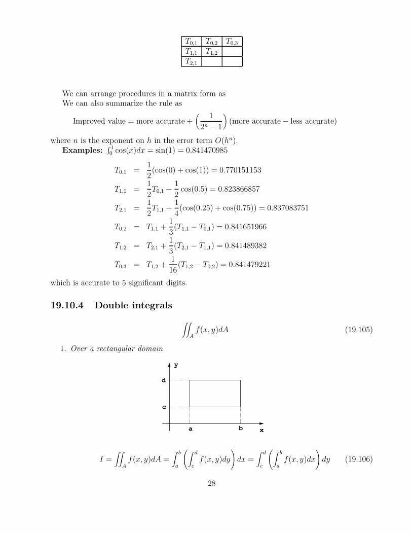
T0,1 T0,2 T0,3
T1,1 T1,2
T2,1
We can arrange procedures in a matrix form asWe can also summarize the rule as
Improved value = more accurate +(
1
2n − 1
)
(more accurate − less accurate)
where n is the exponent on h in the error term O(hn).Examples:
∫ 10 cos(x)dx = sin(1) = 0.841470985
T0,1 =1
2(cos(0) + cos(1)) = 0.770151153
T1,1 =1
2T0,1 +
1
2cos(0.5) = 0.823866857
T2,1 =1
2T1,1 +
1
4(cos(0.25) + cos(0.75)) = 0.837083751
T0,2 = T1,1 +1
3(T1,1 − T0,1) = 0.841651966
T1,2 = T2,1 +1
3(T2,1 − T1,1) = 0.841489382
T0,3 = T1,2 +1
16(T1,2 − T0,2) = 0.841479221
which is accurate to 5 significant digits.
19.10.4 Double integrals
∫∫
Af(x, y)dA (19.105)
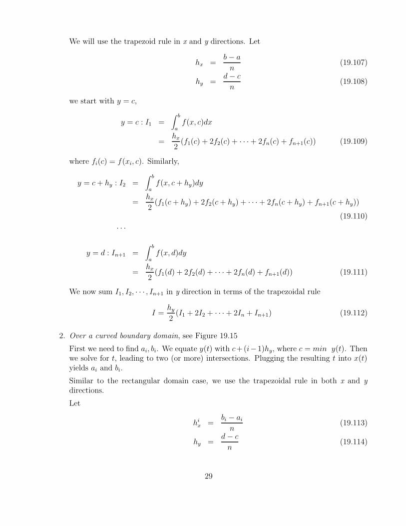
1. Over a rectangular domain
x
y
a b
c
d
I =∫∫
Af(x, y)dA =
∫ b
a
(
∫ d
cf(x, y)dy
)
dx =∫ d
c
(
∫ b
af(x, y)dx
)
dy (19.106)
28
We will use the trapezoid rule in x and y directions. Let
hx =b − a
n(19.107)
hy =d − c
n(19.108)
we start with y = c,
y = c : I1 =∫ b
af(x, c)dx
=hx
2(f1(c) + 2f2(c) + · · · + 2fn(c) + fn+1(c)) (19.109)
where fi(c) = f(xi, c). Similarly,
y = c + hy : I2 =∫ b
af(x, c + hy)dy
=hx
2(f1(c + hy) + 2f2(c + hy) + · · · + 2fn(c + hy) + fn+1(c + hy))
(19.110)
· · ·
y = d : In+1 =∫ b
af(x, d)dy
=hx
2(f1(d) + 2f2(d) + · · · + 2fn(d) + fn+1(d)) (19.111)
We now sum I1, I2, · · · , In+1 in y direction in terms of the trapezoidal rule
I =hy
2(I1 + 2I2 + · · ·+ 2In + In+1) (19.112)
2. Over a curved boundary domain, see Figure 19.15
First we need to find ai, bi. We equate y(t) with c+(i−1)hy, where c = min y(t). Thenwe solve for t, leading to two (or more) intersections. Plugging the resulting t into x(t)yields ai and bi.
Similar to the rectangular domain case, we use the trapezoidal rule in both x and ydirections.
Let
hix =
bi − ai
n(19.113)
hy =d − c
n(19.114)
29
������������������������������������������������������������������������������������������������������������������������������������������������������������������������������������������������������������������������������������������������������������������������������������������������������������������������������������
x
y
a1a2
an+1
b1 b2
bn+1
C(t)=(x(t),y(t))
d
c
Figure 19.15: A curved boundary domain
We start with y = c:
y = c : I1 =∫ b1
a1
f(x, c)dx
=h1
x
2(f1(c) + 2f2(c) + · · ·+ 2fn(c) + fn+1(c)) (19.115)
y = c + hy : I2 =∫ b2
a2
f(x, c + hy)dx
=h2
x
2(f1(c + hy) + 2f2(c + hy) + · · · + 2fn(c + hy) + fn+1(c + hy))
(19.116)
· · ·
y = d : In+1 =∫ bn+1
an+1
f(x, d)dx
=hn+1
x
2(f1(d) + 2f2(d) + · · ·+ 2fn(d) + fn+1(d)) (19.117)
These formulae can be extended to curved domain boundaries bounding multiply con-nected domains.
30
Bibliography
[1] L. Bardis and N. M. Patrikalakis. Topological structures for generalized boundary repre-sentations. MITSG 94-22, MIT Sea Grant College Program, Cambridge, Massachusetts,September 1994.
[2] E. Brisson. Representing geometric structures in d dimensions: Topology and order.Discrete and Computational Geometry, 9:387–426, 1993.
[3] G. Dahlquist and A. Bjorck. Numerical Methods. Prentice-Hall, Inc., Englewood Cliffs,NJ, 1974.
[4] D. P. Dobkin and M. J. Laszlo. Primitives for the manipulation of three-dimensionalsubdivisions. In Proceedings of the Third ACM Symposium on Computational Geometry,pp. 86–99, Waterloo, Canada, June 1987.
[5] D. P. Dobkin and M. J. Laszlo. Primitives for the manipulation of three-dimensionalsubdivisions. Algorithmica, 4:3–32, 1989.
[6] L. Guibas and J. Stolfi. Primitives for the manipulation of general subdivisions and thecomputation of Voronoi diagrams. ACM Transactions on Graphics, 4(2):74–123, April1985.
[7] F. B. Hildebrand. Advanced Calculus for Applications. Prentice-Hall, Inc., EnglewoodCliffs, New Jersey, 1976.
[8] C. M. Hoffmann. Geometric and Solid Modeling: An Introduction. Morgan KaufmannPublishers, Inc., San Mateo, California, 1989.
[9] G. M. Hunter and K. Steiglitz. Operations on images using quad trees. IEEE Transactionson Pattern Analysis and Machine Intelligence, 1(2):145–153, 1979.
[10] Y. T. Lee and A. A. G. Requicha. Algorithms for computing the volume and other integralproperties of solid objects, I: Known methods and open issues. Communications of theACM, 25(9):635–641, September 1982.
[11] M. Mantyla. An Introduction to Solid Modeling. Computer Science Press, Rockville,Maryland, 1988.
[12] D. Meagher. Geometric modeling using octtree encoding. Computer Graphics and ImageProcessing, 19:129–147, June 1982.
31

[13] M. E. Mortenson. Geometric Modeling. John Wiley and Sons, New York, 1985.
[14] A. A. G. Requicha. Representations of solid objects - theory, methods and systems. ACMComputing Surveys, 12(4):437–464, December 1980.
[15] V. Shapiro. Solid modeling. In G. Farin et al., editor, Handbook of Computer AidedGeometric Design, Chapter 20, pp. 473–518. Elsevier, Amsterdam, 2002.
[16] R. Yagel, D. Cohen, and A. Kaufman. Context sensitive normal estimation for volumeimaging. In N. M. Patrikalakis, editor, Scientific Visualization of Physical Phenomena,pp. 211–232. Tokyo: Springer-Verlag, 1991.
32

![13.472J/1.128J/2.158J/16.940J COMPUTATIONAL GEOMETRY · surfaces [14, 11]. 20.1.1 Motivation • ship design • robot motion planning • terrain navigation • installation of underwater](https://img.pdfslide.net/doc/110x75/5f651a0da7ee0937cf7a26a0/13472j1128j2158j16940j-computational-geometry-surfaces-14-11-2011-motivation.jpg)