1388 IEEE TRANSACTIONS ON BIOMEDICAL ENGINEERING, … · family of 2-D methods proposes to segment speciﬁc anatomi-cal structures with morphological operators, ... detailed manual

1388 IEEE TRANSACTIONS ON BIOMEDICAL ENGINEERING, VOL. 60, NO. 5, MAY 2013

Automatic Segmentation of Antenatal3-D Ultrasound Images

Jeremie Anquez, Elsa D. Angelini, Senior Member, IEEE, Gilles Grange, and Isabelle Bloch∗, Member, IEEE

Abstract—The development of 3-D ultrasonic probes and 3-Dultrasound (3DUS) imaging offers new functionalities that call forspecific image processing developments. In this paper, we proposean original method for the segmentation of the utero-fetal unit(UFU) from 3DUS volumes, acquired during the first trimester ofgestation. UFU segmentation is required for a number of tasks,such as precise organ delineation, 3-D modeling, quantitative mea-surements, and evaluation of the clinical impact of 3-D imaging.The segmentation problem is formulated as the optimization of apartition of the image into two classes of tissues: the amniotic fluidand the fetal tissues. A Bayesian formulation of the partition prob-lem integrates statistical models of the intensity distributions ineach tissue class and regularity constraints on the contours. An en-ergy functional is minimized using a level set implementation of adeformable model to identify the optimal partition. We propose tocombine Rayleigh, Normal, Exponential, and Gamma distributionmodels to compute the region homogeneity constraints. We testedthe segmentation method on a database of 19 antenatal 3DUS im-ages. Promising results were obtained, showing the flexibility ofthe level set formulation and the interest of learning the most ap-propriate statistical models according to the idiosyncrasies of thedata and the tissues. The segmentation method was shown to berobust to different types of initialization and to provide accurateresults, with an average overlap measure of 0.89 when comparingwith manual segmentations.

Index Terms—Antenatal imaging, biomedical image processing,image segmentation, level sets, 3-D ultrasonic imaging.

I. INTRODUCTION AND LITERATURE

U LTRASOUND imaging, introduced for obstetrical screen-ing in the 1950s, became widely used as a diagnostic tool

in the late 1960s, and was introduced as a screening tool for preg-nancy monitoring in the late 1970s [1]. It remains the modalityof choice for routine fetal imaging [2]. Obstetrical echographycovers several applications including precise determination ofthe pregnancy stage, placenta positioning, fetal growth, or char-

Manuscript received April 23, 2012; revised August 25, 2012, November 9,2012, and December 27, 2012; accepted December 27, 2012. Date of publi-cation January 1, 2013; date of current version April 15, 2013. This work wassupported in part by Orange Labs R&D and Fondation Sante et Radiofrequences(FEMONUM Project). Asterisk indicates corresponding author.

J. Anquez is with Theraclion, 92240 Malakoff, France (e-mail:[email protected]).

E. D. Angelini is with the Institut Mines-Telecom, Telecom ParisTech, CNRSLTCI, 75013 Paris, France (e-mail: [email protected]).

G. Grange is with the Maternite Port Royal AP-HP, Groupe Hos-pitalier Cochin Saint Vincent De Paul, 75014 Paris, France (e-mail:[email protected]).

∗I. Bloch is with the Institut Mines-Telecom, Telecom ParisTech, CNRSLTCI, 75013 Paris, France (e-mail: [email protected]).

Color versions of one or more of the figures in this paper are available onlineat http://ieeexplore.ieee.org.

Digital Object Identifier 10.1109/TBME.2012.2237400

acterization of potential pathologies [3]. Standard echographyscreening includes the acquisition of a series of 2-D B-scananatomical images. These images are used for visual inspec-tion or to perform quantitative measures of biometric markerssuch as biparietal diameter, femur length, head circumference,or abdominal circumference [4]. Three-dimensional echogra-phy was introduced in the early 1990s for fetal screening, but itswidespread was limited due to poor image quality and slow ac-quisition protocols, unable to prevent fetal motion artifacts [5].These limitations are progressively disappearing with advancedtechnologies, increasing the clinical interest for 3-D ultrasound(3DUS) [6]. During the first trimester and early stage of thesecond trimester of gestation, the field of view of the ultrasoundprobes can integrate the whole gestational sac. Consequently,3DUS-based volumetric studies of uterine structures have beenpublished [7], as well as quantification of the whole fetus [8] orpartial body portions (e.g., head and trunk) [9], providing usefulinformation for clinical routine. These volumetric studies stillrely on manual tracing, and automated segmentation methodsare, therefore, desirable. Semi-automated methods were used inrecent studies, especially with the software tool VOCAL, com-mercialized by General Electric and cited in several works [7],[9], [10]. It enables to reconstruct smooth organ surfaces froma set of 2-D contours acquired on rotated views along a singleaxis [11]. This software remains limited to the extraction of sin-gle organs and is not yet capable of segmenting complex objectssuch as the whole fetus. Moreover, several manual interactionsare often needed. Other works have dealt with the segmenta-tion of specific organs, such as the cardiac cavities [12], using acommercial segmentation tool, and manually supervised imagepartition.

The general domain of automated ultrasound image segmen-tation was reviewed in [13] and includes dedicated methods forthe extraction of biometric markers on fetal US imaging. A firstfamily of 2-D methods proposes to segment specific anatomi-cal structures with morphological operators, such as the femurin [14], and the skull in [15]. A second family of methods isbased on deformable models. A parametric active contour [16],exploiting local intensity variations, was used in [17] to seg-ment the skull. This approach was limited by the requirementsto initialize the contour close to the skull borders and the lackof robustness on images with poor skull contrast. In [18], aBayesian parametric deformable model was proposed, exploit-ing statistical models of intensity distributions in the femoraland skull bones. Recent works in [19] have enabled the segmen-tation of the skull, abdomen, and femoral bone.

Few works were dedicated to automated segmentation of3DUS images for obstetrical applications, although there is

0018-9294/$31.00 © 2013 IEEE

ANQUEZ et al.: AUTOMATIC SEGMENTATION OF ANTENATAL 3-D ULTRASOUND IMAGES 1389

a real clinical need for automated and reproducible methodsleading to reliable quantitative measurements. We can cite thepreliminary work of Sarti et al. [20] where the so-called sub-jective surfaces were proposed to segment objects with partiallymissing contours. In [21], these surfaces were improved withadditional homogeneity terms, to segment fetal heart cavities ontwo datasets. More recently, the method proposed in [22] usesa maximum likelihood (ML) formalism optimized with levelset deformable models. Intensities inside and outside the fetuswere modeled with Rayleigh distributions, but no clinical vali-dation of the method was reported. In [23], the authors deriveda multiple object detection framework evaluated on 3DUS fe-tal ultrasound for brain structures and faces. Binary classifiers,indicating the presence or absence of an object, were learnedfrom a large database of annotated images. In [24], the authorsproposed a method for fetal face extraction from 3DUS data.Multiscale Haar expansions and steerable filters were used toderive image features on face landmark points. The same fea-tures were used in [25] for the supervised learning and detectionof fetal anatomical structures.

In this paper, we address the problem of fetal 3DUS vol-ume segmentation as an optimal partition of the voxels intostatistically “homogeneous” regions (corresponding to differentclasses) with smooth contours. We use parametric probabilitydistribution functions (pdf) to measure region homogeneities,as in [22]. The classification task is formulated as a variationaldeformable model segmentation, within a level set framework,and performed through an iterative deformation process of aninitial shape. As an original feature of the method, we propose torely on a generic class of pdf which can model different types oftissue distributions in both saturated and non-saturated images.This differs from existing methods such as [22]–[25].

Segmentation results were evaluated quantitatively with thehelp of an experienced obstetrician, who provided some manualsegmentations. Experiments on 19 obstetrical ultrasound 3-Dimages illustrate the behavior of the method and the influenceof the parameters. Quantitative results show accurate and robustsegmentation performances.

II. 3DUS IMAGES AND TISSUE APPEARANCE MODELS

A. Image Database

A database of 3DUS volumes (noted DB = {Ii}i=1...19) wasgathered, including:

1) eighteen 3-D volumes {Ii}i=1...18 provided by the Beau-jon AP-HP hospital (Clichy, France) and acquired with aVoluson 730 Expert system from General Electric (GE,Zipf, Austria), with a 3.7–9.3 MHz transvaginal volumet-ric probe. Spatial resolution ranges from 0.21 to 0.96 mm3

with isotropic voxels;2) and one 3-D volume I19 provided by Philips Healthcare

Research Labs (Suresnes, France) and acquired with aiU22 transducer from Philips Ultrasound (Bothell, WA,USA), with a 2-6 MHz volumetric probe. Spatial resolu-tion was 0.95 × 0.6 × 1.37 mm3 .

This database enabled us to study a large set of examplesof fetuses in different positions and at different stages of ges-

tation during the first trimester of pregnancy. All cases in thedatabase were associated with their timing of acquisition, mea-sured as the number of weeks of amenorrhea (WA) of the mother,which ranged between 8 and 13 WA for {Ii}i=1...18 . The ad-ditional case, I19 , acquired at 22 WA, was also included in thedatabase. Voluson images were acquired using harmonic imag-ing and without compounding. This corresponds to the routineacquisition mode used at the collaborating hospital for obstetric3DUS acquisitions during the first trimester, to optimize im-age contrast at the interfaces between tissues. The echographersdefined a field of view as small as possible, while includingthe whole amniotic sac. In some cases, the amniotic sac was,however, slightly truncated. Images were post-processed (forspeckle reduction) and reconstructed on a Cartesian grid withdedicated post-processing tools provided by the manufacturersand included in the ultrasound scanning systems. Voxel intensi-ties were normalized during this process in the range of values[0, 255]. These considerations have an impact on the modelingof the intensity distributions, as explained later.

Given the low signal-to-noise ratio (SNR) of ultrasound im-age data, setting up an automated segmentation of homogeneousstructures is a difficult task. Indeed, images are corrupted withtextured speckle noise and some structures lack sharp contrastalong their contours. Visual inspection of the data by an obste-trician relies heavily on prior knowledge of the fetal anatomy,and the specific image characteristics generated by the presenceof highly reflective interfaces, absorption in bone structures,and echo cancellation along interfaces parallel to the ultrasoundbeam. To learn tissue appearance and validate the segmentationmethod presented in this paper, an experienced obstetrician in-teractively processed the images with two different approaches:1) detailed manual segmentation of some fetal and maternalstructures, 2) binarization of the images into amniotic fluid andfetal tissues via intensity thresholding. These two approachesare now detailed.

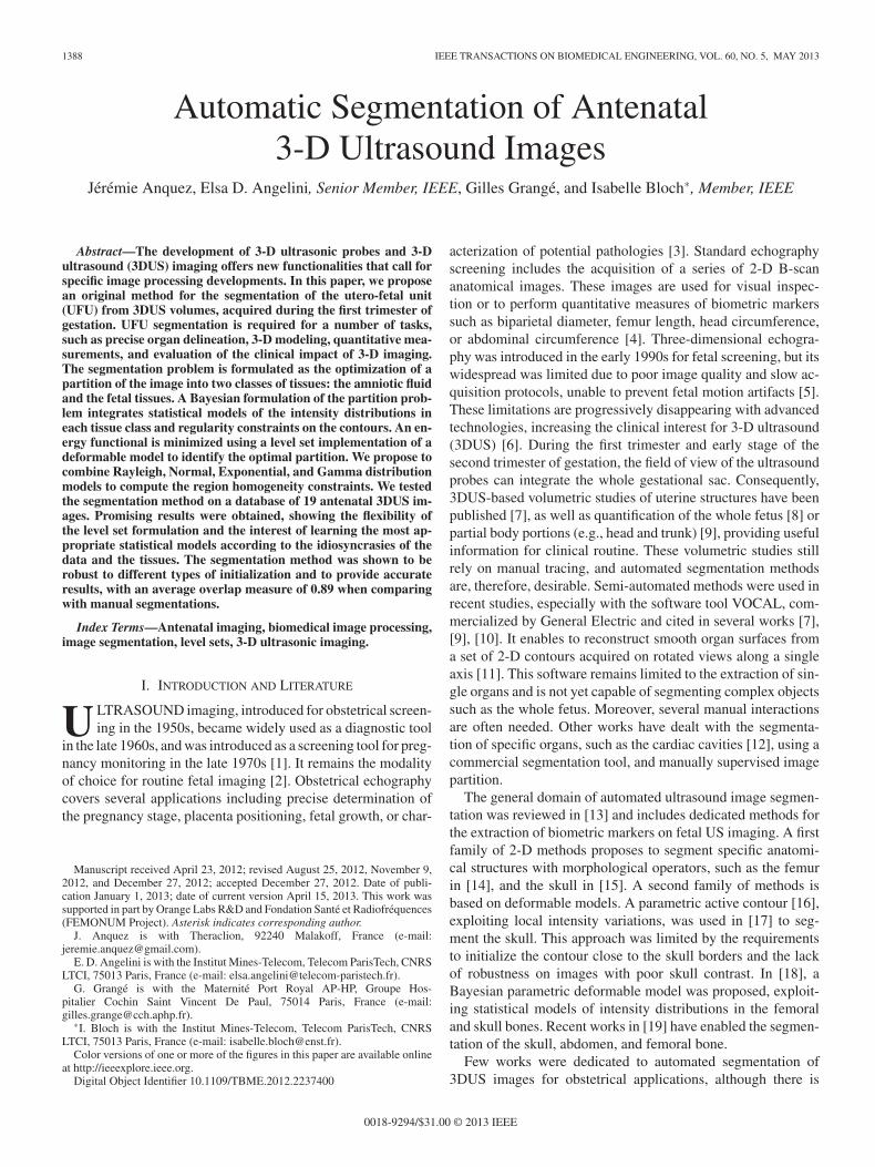
1) Manual segmentation of 3DUS volumes is a tedious taskgiven their large size and their low SNR. Therefore, only asubset of five volumes was manually segmented in 3-D. Theset of volumes included four development stages of the fetusesover the first trimester, corresponding to 8-9-10-13 WA, and thecase at 22 WA. The placenta, amniotic fluid, fetus envelope,and umbilical cord were manually delineated by an experiencedobstetrician. Slices from the 9 and 13 WA cases are illustrated inFig. 1(a) and (b), with the corresponding detailed manual seg-mentations. For the other volumes of the database, three slicesin orthogonal directions were segmented to outline the spatialextent of the anatomical structures of interest. Two voxel classeswere distinguished: the amniotic fluid and the fetal tissues (in-cluding the placenta,1 umbilical cord, and fetus), as illustratedin Fig. 1(c) and (d). The two classes, included in these partialsegmentations, are denoted AF and FT, respectively.

2) Using an interactive software tool, the experienced ob-stetrician interactively defined for each volume case-specificthreshold values to binarize the volumes into two regions, cor-responding to AF and FT.

1The placenta is indeed a fetal tissue originating from the feconded egg.


Fig. 1. (a) and (b) Two-dimensional slices of I9 (9 WA), I18 (13 WA) withthe corresponding complete manual segmentations. Segmented tissues are theplacenta (red), the amniotic fluid (blue), the fetus (pink), and the umbilical cord(green). (c) and (d) Two orthogonal slices of I6 (9 WA) with the correspondingpartial manual segmentations. Identified tissues are the amniotic fluid (gray)and fetal tissues (white).

Our segmentation framework is designed to be used with anytype of initialization (e.g., random–uniform partitions or thresh-olding with an a priori threshold). We used the manually definedthresholds to learn an average threshold value, that can be usedfor the initial partition of any new volume of images to segment,prior to fine level-set segmentation. This initialization greatlyspeeds up the convergence of the segmentation algorithm. Twocriteria were considered to define the manual threshold values:1) the completeness of the boundary between the placenta andthe amniotic fluid, and 2) the precision of the position of theboundary between the fetus and the amniotic fluid. A first set ofthreshold values {s1

i } was defined for each volume of images Ii

during a first session. One week later, a second session was heldto identify a second set of values {s2

i }. These consecutive ses-sions enabled us to assess the intra-expert variability in defininga single optimal threshold value per case. The mean value si

between the two experiments was computed. Let εi = |s1i − s2

i |be the absolute difference between the two thresholds for eachIi . Let με and σε be the mean and standard deviation of the εi

values, respectively. A noticeable intra-user variability was mea-sured, since με = 12.8 and σε = 5.6, which can be explainedby the important amount of noise in the images. The quantityε+ = maxi(εi) can be used to define an interval of “admissible”threshold values for each volume of the database: a value s isconsidered admissible to binarize Ii if it satisfies s ∈ [s−i , s+

i ],with s+

i = si + ε+

2 and s−i = si − ε+

2 . Let μsi be the average

of the mean threshold values si over the whole database butexcluding the volume Ii . These average values μs

i ended upto be admissible threshold values for 17 of the 19 volumes ofimages of the database. For the other two volumes, the averagestill remained close to the si values (less than five gray levelsdifference).

Alternative threshold values were also studied, using theOtsu’s automatic thresholding method [26] and the K-meansclassification [27] with K = 2. The same threshold values wereobtained with the two automated selection methods. Let oi bethe threshold value for Ii . The oi threshold values were higherthan the si values and were non-admissible (in a strict sense) in17 of the 19 cases. However, the distances |oi − si | remainedsmall compared to the intensity range in the images (the average

|oi − si | distance was inferior to 25, which is equivalent to 10%of the whole intensity range).

B. Intensity Distribution Modeling

Distributions of voxel intensities were learned based on themanual segmentation presented above. Two sets of voxels wereconsidered: ΩAF , for the voxels belonging to AF, and ΩFT , forthe voxels belonging to FT. During the ultrasound data acquisi-tion process, a transfer function can be applied to saturate the lowand high intensities, reducing the range of attenuations to recordand facilitating image interpretation by the clinician, within softtissues. As a result, some images of the database were saturatedby the ultrasound scanning machine during the acquisition. Wetherefore distinguished two subsets within the database: DBS

which contains saturated volumes and DBS which contains thenon-saturated volumes. This was simply done by identifyingthe presence of an initial large peak in the histogram for satu-rated cases. In this study, histograms were reviewed manuallyto detect the presence of this peak and label each case in thedatabase as having saturated or unsaturated intensities in theamniotic fluid. We identified DBS = {Ii}, i ∈ {1, . . . , 5} andDBS = {Ii}, i ∈ {6, . . . , 19}. Histograms of the intensity val-ues within ΩAF and ΩFT are noted pAF

i and pFTi for the volume

Ii , and can differ significantly.Standard modeling of tissue intensity distributions in US im-

ages has been based on the Rayleigh distribution in many works.However, it did not provide satisfying modeling on our databaseand may not properly model tissue intensities on clinical ultra-sound images as discussed below. Alternatively, we propose toexploit the Gamma distribution, which pdf is expressed as

pG (I(x)) = I(x)α−1 βα exp (−βI(x))Γ(α)

(1)

with I(x) the image intensity at voxel x (with I(x) > 0), α >0, β > 0, and

Γ(α) =∫ ∞

0tα−1e−tdt. (2)

This pdf provides great genericity and flexibility for the mod-eling of voxel intensities, through the parameters α and β. TheML estimators αML and βML of the distribution parameters αand β were evaluated for each dataset. Since no close form existsfor αML , this value was estimated using the method presentedin [28], based on the iterative Newton’s technique. The value ofβML was then computed, which depends only on αML .

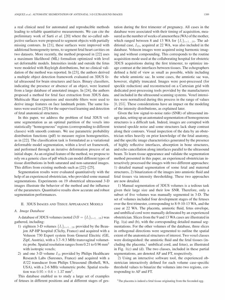
Modeling of the intensity distributions using the Gamma pdfis illustrated in Fig. 2. The histograms pAF

4 (a), pFT4 (b), pAF

13(c), and pFT

13 (d) are displayed, along with the correspondingpdf pG (I(x)) (I4 corresponds to a non-saturated volume, whileI13 is a saturated one). The fitting ability of the distributionis not surprising in the non-saturated case. It was also usedadvantageously in [29] to model blood appearance (a physio-logical fluid with a similar appearance to the amniotic fluid)and soft tissue appearance on echocardiographic images. Moreinterestingly, its genericity also enables to model the intensitieswhen saturated images are considered as illustrated in Fig. 2(c)


Fig. 2. Modeling of the intensity distributions with the Gamma pdf in ΩAFand ΩFT : (a), (b) in the non-saturated volume I4 and (c), (d) in the saturatedvolume I13 . The histograms: (a) pAF

4 , (b) pFT4 , (c) pAF

13 , and (d) pFT13 are

represented in blue and the Gamma distribution pG (I(x)) in green.

and (d). This shows that the Gamma distribution can be usedas a generic intensity model for the AF and the FT, whateverpost-processing was applied to the US signal when recorded bythe scanning system, but at the cost of computing distributionparameters that do not have analytical expressions.

As an alternative, we investigated the use of tissue-specificdistribution models, with analytical ML estimators of the pa-rameters. Depending on the intensity saturation, we propose touse different parametric distributions, dedicated to the two spe-cific tissue types being studied (amniotic fluid or fetal tissues).Regarding the amniotic fluid, we exploit the Rayleigh distribu-tion to model the intensity distribution in non-saturated images.This distribution, initially proposed in [30] and [31], has beenwidely used for ultrasound images processing [13]. The pdf ofthis distribution is expressed as:

pR (I(x)) =I(x) exp

(−I (x)2

2σ 2

)

σ2 (3)

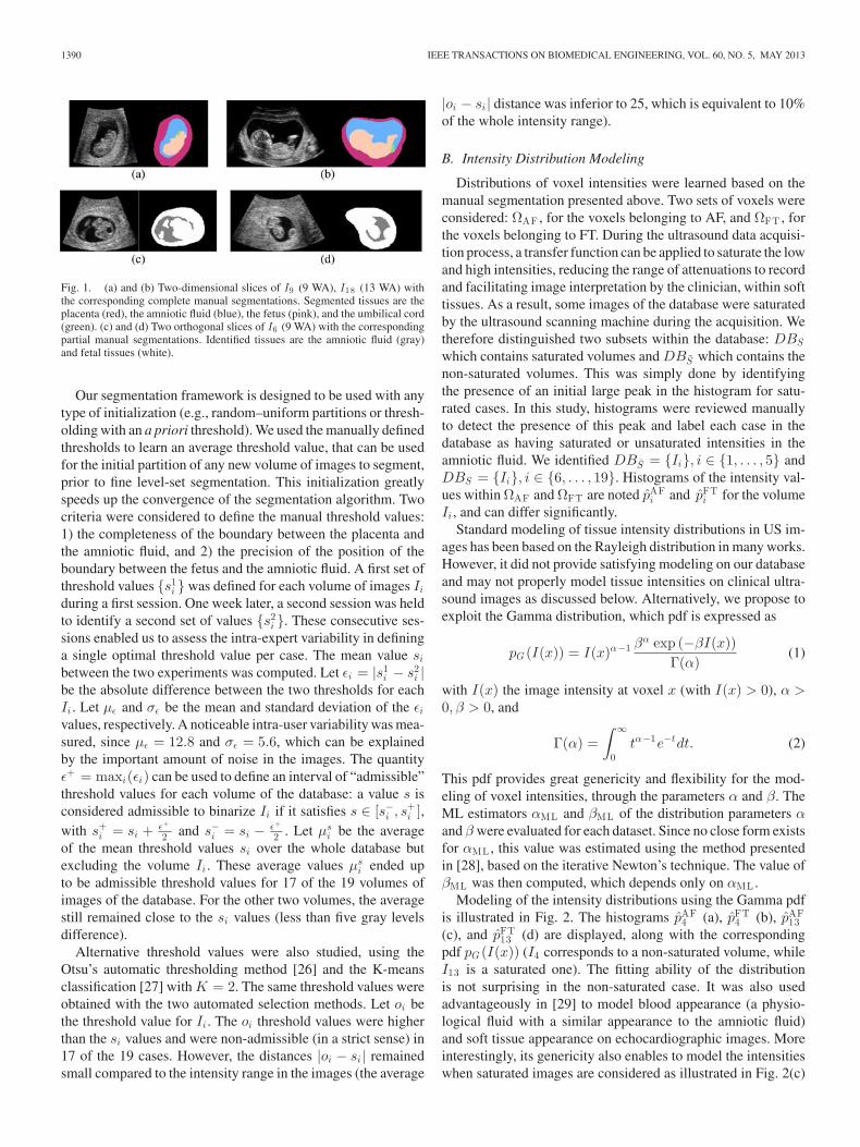
with I(x) ∈ [0,∞) and σ > 0. This distribution provides a goodfit of the intensity distribution in the amniotic fluid of a non-saturated image, as illustrated in Fig. 3(a). However, this isno longer true when the intensities are saturated. In this case,the frequency of the zero intensity class is artificially high.Consequently, the Rayleigh distribution is not relevant sinceit always leads to pR (0) = 0. Moreover, the histogram valuedecreases, while pR (I(x)) increases for I(x) ∈ [0, σ] and de-creases for I(x) ∈ [σ,∞). As a surrogate, we exploit the Expo-nential distribution to model the intensity histograms in ΩAF ,when Ii ∈ DBS . The pdf of this distribution is expressed as:

pE (I(x)) = λe−λI (x) (4)

with I(x) ∈ [0,∞) and λ > 0. This choice clearly fits betterthe intensity histograms than the Rayleigh distribution [see

Fig. 3. Modeling of the intensity distributions with specific models in ΩAFand ΩFT (a), (b) in the non-saturated image I4 and (c), (d) in the saturated imageI13 . The histograms (a) pAF

4 , (b) pFT4 , (c) pAF

13 , and (d) pFT13 are represented

in blue and the Rayleigh distribution pR (I(x)) in cyan (a)–(d). (b), (d) Normaland (c) Exponential distributions are represented in red.

Fig. 3(c)]. This distribution has been seldom considered tomodel intensity distributions in ultrasound images, since sat-urated images are frequently excluded from the test databasesused to validate image processing methods [29]. It has neverthe-less been exploited to model the blood and to segment echocar-diographic images [32]. Regarding fetal tissues, one can noticeby observing pFT

4 and pFT13 in Fig. 3(b) and (d) that there are

very few pixels with intensity below 25, which actually belong toregions affected by acoustic shadowing. Generally, the pFT

i in-crease rate is slow for low intensities. The Rayleigh distributionis therefore not satisfying to model the intensity distributions inΩFT , and we propose to use the Normal distribution. The pdf ofthis distribution is expressed as

pN (I(x)) =1

σ√

2πexp

(− (I(x) − μ)2

2σ2

)(5)

with I(x) ∈ R, μ ∈ R, σ > 0. It was also used to model the in-tensity distribution in soft tissues, to process ultrasound imagesof the heart and prostate in [33] and [34].

An important advantage of the Rayleigh, Exponential, andNormal distributions over the Gamma distribution is that closeforms of the ML estimators of their parameters systematicallyexist. This simplifies the fitting process, in comparison with thecomputation of the Gamma distribution parameter αML , whichis obtained through an iterative process. Choice is left to theuser to give priority either to the genericity of the model or tothe computation speed.

To quantitatively evaluate the goodness of fit between thehistograms and our models, we used the Cramer–Von Misescriterion [35] on the whole database DB and for the twoclasses of tissues. This criterion, CVM, is expressed as CVM =∫ +∞−∞ (P ∗(g) − P (g))2dP (g), comparing the cumulative


TABLE IDESCRIPTION OF THE INTENSITY DISTRIBUTION MODELING STRATEGIES USED

TO GUIDE THE SEGMENTATION OF THE 3DUS VOLUMES

density function of the theoretical distribution P with thecumulative histogram of the empirical data P ∗. This test hasthe advantage of being weakly sensitive to the tail of thedistributions. Since this tail may not be well represented inthe experimental data, and thus wrongly estimated, it is betterto use a test that is not too sensitive to it. The CVM testwas therefore preferred to the Kolomogorov–Smirnov one,which is more sensitive to outliers and wrong estimation ofthe tail of the distribution. The lower the CVM test value, thebetter the fit between the data and the distribution model. Weobtained optimal test values with the Gamma model, followedby the Exponential (for AF)/Normal (for FT) model and theRayleigh model. Average CVM test values for {AF, FT} tissueswith the three models were: {0.001, 0.001} for the Gammamodel, {0.01, 0.001} for the Exponential/Normal model and{0.037, 0.0075} for the Rayleigh model. For the Rayleighmodel, we observed a large variability of the CVM values overthe 19 cases, and the maximum values were 0.08 and 0.02 forAF and FT tissues.

This statistical evaluation confirmed that the Gamma distribu-tion provides a relevant intensity modeling in ΩAF and ΩFT , forsaturated and unsaturated images. Fitting accuracy was equiv-alent or better than with specific distributions in ΩAF , whilebeing slightly inferior than with the Normal distribution for 15cases of the DB in ΩFT .

The segmentation process presented in the next section relieson intensity distributions modeling in ΩAF and ΩFT , whichrequires iterative data fitting and parameters estimation. Theresults obtained with the dedicated models will be comparedwith a strategy consisting in modeling voxels intensities in agiven region using Normal distributions with identical standarddeviations. This model corresponds to the Chan–Vese methoddescribed in [36].

The intensity distribution modeling strategies used to guidethe segmentation process are summarized in Table I. Note thatif using the SD modeling strategy (with distributions dependingon the tissues), information on the presence of saturation ornot is used to decide on using an Exponential or a Rayleighdistribution to model the amniotic fluid.

III. SEGMENTATION METHOD: BAYESIAN FORMULATION AND

VARIATIONAL APPROACH

Let Ω be an open and bounded subset of RN and letI : Ω → R be an N-D image to segment. We propose a methodwhich aims at providing an optimal partition of the image do-main, notedP(Ω) = {Ωe ,Ωi}, by embedding prior informationregarding the distributions followed by the voxel intensities inΩe and Ωi and on the boundary between these two regions (Ωi

and Ωe correspond to ΩAF and ΩFT ). To achieve this task,we consider a Bayesian framework and propose to maximizethe posterior probability of the partition given the image I , de-noted p(P(Ω)|I). Since p(I) is identical for all partitions, thisis equivalent to maximizing p(I|P(Ω))p(P(Ω)). The first termis called the image likelihood and the second term representsthe a priori probability of the partition and is modeled as aboundary smoothness constraint. Maximization of p(P(Ω)|I)corresponds to the identification of the maximum a posteriori(MAP) partition P(Ω).

A. Formulation of the Boundary Smoothness Constraint

Let C be the boundary of the partition P(Ω). Integrating aprior on the boundary enables to regularize the optimizationproblem. This is particularly important in the case of US im-ages, as underlined, for example, in [37]. We aim at modelingsmooth boundaries, since this feature characterizes most organsand anatomical structures. To obtain smooth boundaries, weconsider the following prior that depends on the measure |C| ofthe boundary C (curve in 2-D, surface in 3-D) between Ωe andΩi (i.e. the length in 2-D and the surface area in 3-D):

p(P(Ω)) ∝ ν exp(−ν|C|), ν > 0. (6)

The smoothness of the boundary C is controlled by the pa-rameter ν of this distribution. The choice of ν is explained inSection IV-A.

B. Formulation of the Region Likelihood

The likelihood term relies on a homogeneity measure com-puted at each voxel x with intensity I(x) in the image, whichdepends on the region it belongs to. The pdf p(I(x)) then takes afirst form pe with parameter(s) θe in a parameter space Θe , hencedenoted pe(I(x), θe), if x ∈ Ωe , and a second form pi with pa-rameter(s) θi in a parameter space Θi (denoted pi(I(x), θi)), ifx ∈ Ωi . Consequently, we have

p(I(x)) ={

pe(I(x), θe), if x ∈ Ωe , with θe ∈ Θe

pi(I(x), θi), if x ∈ Ωi , with θi ∈ Θi .(7)

Under the hypothesis that the voxel intensities are independentconditionally to P(Ω), we obtain

p(I|P(Ω)) =∏

x∈Ωe

pe(I(x), θe)∏

x∈Ω i

pi(I(x), θi). (8)

C. Posterior Probability

Integrating (6) and (8) into the posterior probability of apartition P(Ω) conditionally to the image leads to:

p(P(Ω)|I)=ν exp(−ν|C|)∏

x∈Ωe

pe(I(x), θe)∏

x∈Ω i

pi(I(x), θi).

(9)

D. Formulation of the MAP Optimization Problem

To solve the MAP problem, we linearize the posterior prob-ability by defining an energy E equal to the negative loga-rithm of p(P(Ω)|I). The negative logarithm function being


strictly decreasing, the minimization of E is equivalent to themaximization of p(P(Ω)|I). Therefore, we look for C, θe , θi

minimizing E:

E(C, θe , θi) = Ereg (C) + Ee(C, θe) + Ei(C, θi) (10)

with ⎧⎪⎨⎪⎩

Ereg (C) = − log ν + ν|C|Ee(C, θe) = −

∫x∈Ωe

log pe(I(x), θe)dx

Ei(C, θi) = −∫

x∈Ω ilog pi(I(x), θi)dx.

Note that the integrals become discrete sums over a boundeddomain in the implementation on digital images. The energyE is minimized by optimizing its three parameters (C, θe , θi),noting that {Ωe ,Ωi} are entirely defined by the position of thecontour C. The constant − log ν of Ereg is neglected in thefollowing, since it depends on a weighting parameter ν that isnot optimized during the minimization process of E, but fixedbeforehand.

E. Segmentation Via Energy Minimization

Minimization of the energy functional E is performed by aniterative process, progressively deforming an initial contour C0and updating the pdf parameters {θe , θi}. At each iteration, thecontour is deformed to correspond to a lower energy level. Toimplement this iterative process, we need to encode the spatiallocalization of the contour C. To do this, we chose to use thelevel set framework which represents the contours C implicitlyas the zero level of a scalar function φ : Ω → R. The sign ofφ therefore defines two regions: Ωe , where φ(x) > 0, and Ωi ,where φ(x) < 0 [38]. The boundary C between Ωe and Ωi isimplicitly defined as φ(x) = 0.

To reformulate the energy functional in terms of φ instead of{Ωe ,Ωi} (or C), we express the measure |C| in Ereg (φ) withthe Dirac function δ(φ), equal to zero everywhere except whereφ(x) = 0. The terms Ee and Ei can be rewritten as integrals overthe entire image, by exploiting the Heaviside function H(φ),equal to 1 where φ(x) > 0 and zero elsewhere. Equation (10)is, therefore, rewritten as:

E(φ, θi, θe) = Ereg (φ) + Ee(φ, θe) + Ei(φ, θi)

with⎧⎪⎨⎪⎩

Ereg (φ) = ν∫

x∈Ω δ(φ(x))|∇φ(x)|dx

Ee(φ, θe) = −∫

x∈Ω H(φ(x)) log(pe(I(x), θe))dx

Ei(φ, θi) = −∫

x∈Ω(1 − H(φ(x))) log(pi(I(x), θi))dx.

The energy E now depends on the three parameters (φ, θe , θi).The minimization of E is performed using the numerical im-plementation detailed in [36]. This implementation alternatesbetween two minimization tasks:

1) minimizing E with respect to θe and θi (with a fixed φ),and

2) minimizing E with respect to φ (with fixed θe and θi

parameters).The energy E being non-convex, only a local minimum

might be obtained [39]. The quality of the initialization might,

TABLE IIML ESTIMATORS θr OF THE PARAMETER VALUES FOR THE PDF LAWS

CONSIDERED IN THE HOMOGENEITY MEASURES [r = e, i]

therefore, play an important role, which is further discussed inSection IV-D.

Starting from an initial function φ0(x) at time t = 0, wedefine φ(x, 0) = φ0(x). This initial function is defined as thesigned distance to the initial contour C0 . A gradient descent isthen used to derive the following system governing the dynamicdeformation of the implicit level set function, now noted φ(x, t):⎧⎪⎪⎪⎪⎪⎪⎨

⎪⎪⎪⎪⎪⎪⎩

θr = arg minθr ∈Θ r

(Er (C, θr ))

= arg minθr ∈Θ r

(−

∫x∈Ωr

log(pr (I(x), θr ))dx

), [r = i, e]

∂φ

∂t= δ(φ(x))(Freg (φ(x)) + Fdata(φ(x), θe , θi)) in Ω

(11)with⎧⎪⎪⎪⎨

⎪⎪⎪⎩

Freg (φ(x)) = νdiv

(∇φ(x)|∇φ(x)|

)

Fdata(φ(x), θe , θi) = Fi(φ(x), θi) − Fe(φ(x), θe)

Fr (φ(x), θr ) = − log pr (I(x), θr ), [r = i, e]

where Freg , Fe , Fi are derived from Ereg , Ee , Ei , respectively,by calculating the partial derivatives with respect to φ.

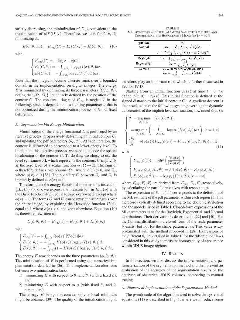
The expression of θr in (11) corresponds to the definition ofthe ML estimate of the pdf parameter within each region Ωr . It istherefore explicitly defined according to the chosen distributionand the models listed in Table I. Closed-form expressions of theML parameters exist for the Rayleigh, Exponential, and Normaldistributions. Their derivation is described in [22] and [40]. Forthe Gamma distribution, a closed form of the scale parameterβ exists, but not for the shape parameter α. This value is ap-proximated with the method proposed in [28]. Expressions ofthe different θr are detailed in Table II for the different pdf lawsconsidered in this study to measure homogeneity of appearancewithin 3DUS image regions.

IV. RESULTS

In this section, we first discuss the implementation and pa-rameterization of the segmentation method and then present anevaluation of the accuracy of the segmentation results on thedatabase of obstetrical 3DUS volumes, comparing to manualtracing.

A. Numerical Implementation of the Segmentation Method

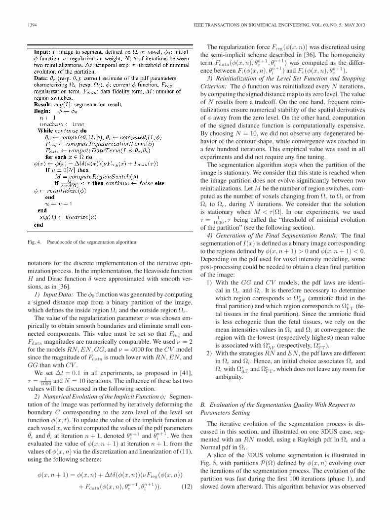
The pseudocode of the algorithm used to solve the system ofequations (11) is described in Fig. 4, where we introduce some


Fig. 4. Pseudocode of the segmentation algorithm.

notations for the discrete implementation of the iterative opti-mization process. In the implementation, the Heaviside functionH and Dirac function δ were approximated with smooth ver-sions, as in [36].

1) Input Data: The φ0 function was generated by computinga signed distance map from a binary partition of the image,which defines the inside region Ωi and the outside region Ωe .

The value of the regularization parameter ν was chosen em-pirically to obtain smooth boundaries and eliminate small con-nected components. This value must be set so that Freg andFdata magnitudes are numerically comparable. We used ν = 2for the models RN,EN,GG, and ν = 4000 for the CV modelsince the magnitude of Fdata is much lower with RN,EN , andGG than with CV .

We set Δt = 0.1 in all experiments, as proposed in [41],τ = 1

1000 and N = 10 iterations. The influence of these last twovalues will be discussed in the following section.

2) Numerical Evolution of the Implicit Function φ: Segmen-tation of the image was performed by iteratively deforming theboundary C corresponding to the zero level of the level setfunction φ(x, t). To update the value of the implicit function ateach voxel x, we first computed the values of the pdf parametersθe and θi at iteration n + 1, denoted θn+1

e and θn+1i . We then

evaluated the value of φ(x, n + 1) at iteration n + 1, from thevalues of φ(x, n) via the discretization and linearization of (11),using the following scheme:

φ(x, n + 1) = φ(x, n) + Δtδ(φ(x, n))(νFreg (φ(x, n))

+ Fdata(φ(x, n), θn+1e , θn+1

i )). (12)

The regularization force Freg (φ(x, n)) was discretized usingthe semi-implicit scheme described in [36]. The homogeneityterm Fdata(φ(x, n), θn+1

e , θn+1i ) was computed as the differ-

ence between Fi(φ(x, n), θn+1i ) and Fe(φ(x, n), θn+1

e ).3) Reinitialization of the Level Set Function and Stopping

Criterion: The φ function was reinitialized every N iterations,by computing the signed distance map to its zero level. The valueof N results from a tradeoff. On the one hand, frequent reini-tializations ensure numerical stability of the spatial derivativesof φ away from the zero level. On the other hand, computationof the signed distance function is computationally expensive.By choosing N = 10, we did not observe any degenerated be-havior of the contour shape, while convergence was reached ina few hundred iterations. This empirical value was used in allexperiments and did not require any fine tuning.

The segmentation algorithm stops when the partition of theimage is stationary. We consider that this state is reached whenthe image partition does not evolve significantly between tworeinitializations. Let M be the number of region switches, com-puted as the number of voxels changing from Ωe to Ωi or fromΩi to Ωe , during N iterations. We consider that the solutionis stationary when M < τ |Ω|. In our experiments, we usedτ = 1

1000 , τ being called the “threshold of minimal evolutionof the partition” (see the following section).

4) Generation of the Final Segmentation Result: The finalsegmentation of I(x) is defined as a binary image correspondingto the regions defined by φ(x, n + 1) > 0 and φ(x, n + 1) < 0.Depending on the pdf used for voxel intensity modeling, somepost-processing could be needed to obtain a clean final partitionof the image:

1) With the GG and CV models, the pdf laws are identi-cal in Ωe and Ωi . It is therefore necessary to determinewhich region corresponds to Ω∗

AF (amniotic fluid in thefinal partition) and which region corresponds to Ω∗

FT (fe-tal tissues in the final partition). Since the amniotic fluidis less echogenic than the fetal tissues, we rely on themean intensities values in Ωe and Ωi at convergence: theregion with the lowest (respectively highest) mean valueis associated with Ω∗

AF (respectively, Ω∗FT ).

2) With the strategies RN and EN , the pdf laws are differentin Ωe and Ωi . Hence, an initial choice associates Ωe andΩi with Ω∗

AF and Ω∗FT , which does not leave any room for

ambiguity.

B. Evaluation of the Segmentation Quality With Respect toParameters Setting

The iterative evolution of the segmentation process is dis-cussed in this section, and illustrated on one 3DUS case, seg-mented with an RN model, using a Rayleigh pdf in Ωe and aNormal pdf in Ωi .

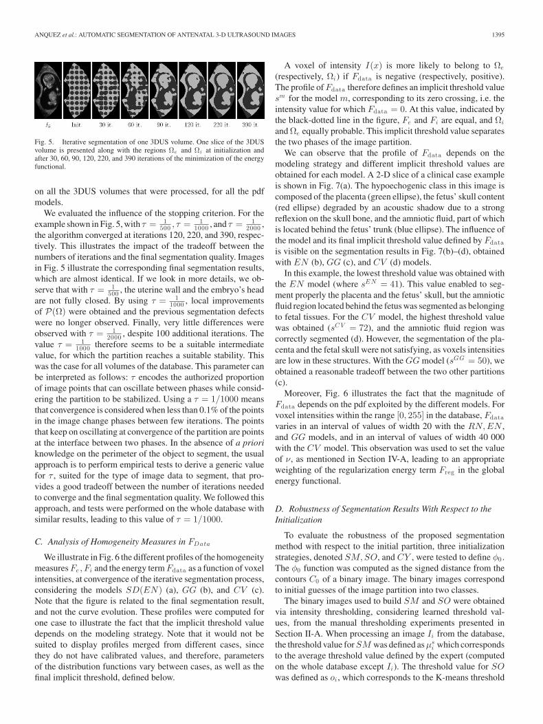
A slice of the 3DUS volume segmentation is illustrated inFig. 5, with partitions P(Ω) defined by φ(x, n) evolving overthe iterations of the segmentation process. The evolution of thepartition was fast during the first 100 iterations (phase 1), andslowed down afterward. This algorithm behavior was observed


Fig. 5. Iterative segmentation of one 3DUS volume. One slice of the 3DUSvolume is presented along with the regions Ωe and Ωi at initialization andafter 30, 60, 90, 120, 220, and 390 iterations of the minimization of the energyfunctional.

on all the 3DUS volumes that were processed, for all the pdfmodels.

We evaluated the influence of the stopping criterion. For theexample shown in Fig. 5, with τ = 1

500 , τ = 11000 , and τ = 1

2000 ,the algorithm converged at iterations 120, 220, and 390, respec-tively. This illustrates the impact of the tradeoff between thenumbers of iterations and the final segmentation quality. Imagesin Fig. 5 illustrate the corresponding final segmentation results,which are almost identical. If we look in more details, we ob-serve that with τ = 1

500 , the uterine wall and the embryo’s headare not fully closed. By using τ = 1

1000 , local improvementsof P(Ω) were obtained and the previous segmentation defectswere no longer observed. Finally, very little differences wereobserved with τ = 1

2000 , despite 100 additional iterations. Thevalue τ = 1

1000 therefore seems to be a suitable intermediatevalue, for which the partition reaches a suitable stability. Thiswas the case for all volumes of the database. This parameter canbe interpreted as follows: τ encodes the authorized proportionof image points that can oscillate between phases while consid-ering the partition to be stabilized. Using a τ = 1/1000 meansthat convergence is considered when less than 0.1% of the pointsin the image change phases between few iterations. The pointsthat keep on oscillating at convergence of the partition are pointsat the interface between two phases. In the absence of a prioriknowledge on the perimeter of the object to segment, the usualapproach is to perform empirical tests to derive a generic valuefor τ , suited for the type of image data to segment, that pro-vides a good tradeoff between the number of iterations neededto converge and the final segmentation quality. We followed thisapproach, and tests were performed on the whole database withsimilar results, leading to this value of τ = 1/1000.

C. Analysis of Homogeneity Measures in FData

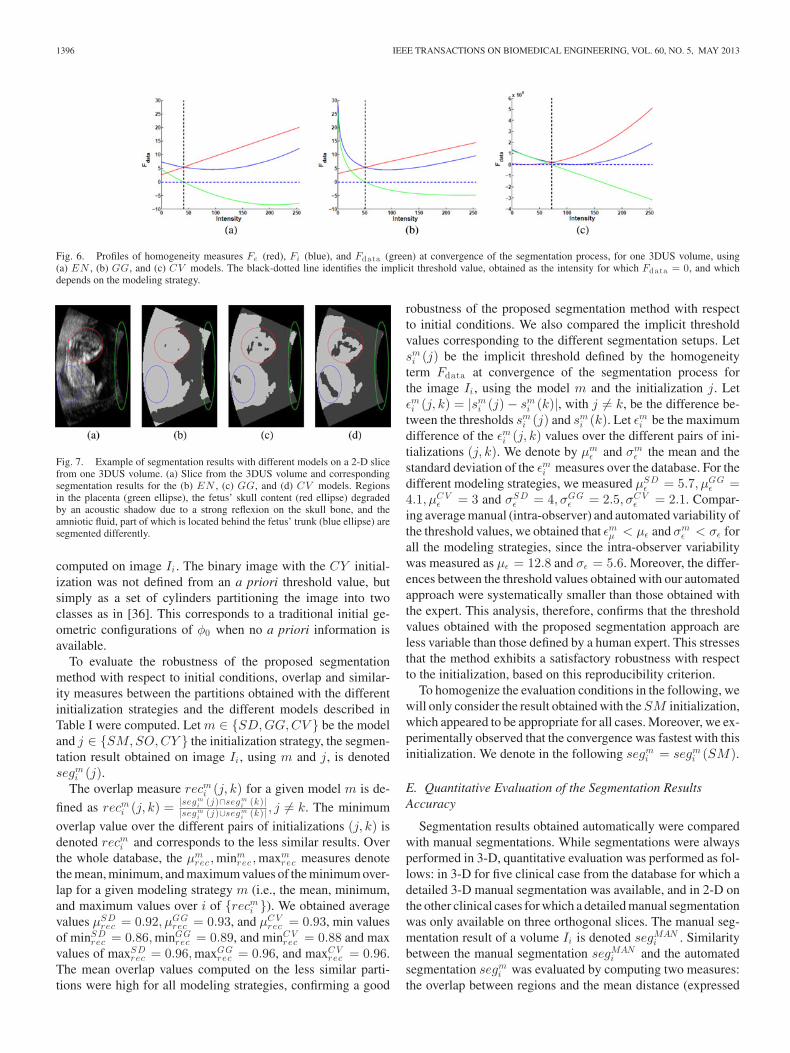
We illustrate in Fig. 6 the different profiles of the homogeneitymeasures Fe, Fi and the energy term Fdata as a function of voxelintensities, at convergence of the iterative segmentation process,considering the models SD(EN) (a), GG (b), and CV (c).Note that the figure is related to the final segmentation result,and not the curve evolution. These profiles were computed forone case to illustrate the fact that the implicit threshold valuedepends on the modeling strategy. Note that it would not besuited to display profiles merged from different cases, sincethey do not have calibrated values, and therefore, parametersof the distribution functions vary between cases, as well as thefinal implicit threshold, defined below.

A voxel of intensity I(x) is more likely to belong to Ωe

(respectively, Ωi) if Fdata is negative (respectively, positive).The profile of Fdata therefore defines an implicit threshold valuesm for the model m, corresponding to its zero crossing, i.e. theintensity value for which Fdata = 0. At this value, indicated bythe black-dotted line in the figure, Fe and Fi are equal, and Ωi

and Ωe equally probable. This implicit threshold value separatesthe two phases of the image partition.

We can observe that the profile of Fdata depends on themodeling strategy and different implicit threshold values areobtained for each model. A 2-D slice of a clinical case exampleis shown in Fig. 7(a). The hypoechogenic class in this image iscomposed of the placenta (green ellipse), the fetus’ skull content(red ellipse) degraded by an acoustic shadow due to a strongreflexion on the skull bone, and the amniotic fluid, part of whichis located behind the fetus’ trunk (blue ellipse). The influence ofthe model and its final implicit threshold value defined by Fdatais visible on the segmentation results in Fig. 7(b)–(d), obtainedwith EN (b), GG (c), and CV (d) models.

In this example, the lowest threshold value was obtained withthe EN model (where sEN = 41). This value enabled to seg-ment properly the placenta and the fetus’ skull, but the amnioticfluid region located behind the fetus was segmented as belongingto fetal tissues. For the CV model, the highest threshold valuewas obtained (sC V = 72), and the amniotic fluid region wascorrectly segmented (d). However, the segmentation of the pla-centa and the fetal skull were not satisfying, as voxels intensitiesare low in these structures. With the GG model (sGG = 50), weobtained a reasonable tradeoff between the two other partitions(c).

Moreover, Fig. 6 illustrates the fact that the magnitude ofFdata depends on the pdf exploited by the different models. Forvoxel intensities within the range [0, 255] in the database, Fdatavaries in an interval of values of width 20 with the RN,EN ,and GG models, and in an interval of values of width 40 000with the CV model. This observation was used to set the valueof ν, as mentioned in Section IV-A, leading to an appropriateweighting of the regularization energy term Freg in the globalenergy functional.

D. Robustness of Segmentation Results With Respect to theInitialization

To evaluate the robustness of the proposed segmentationmethod with respect to the initial partition, three initializationstrategies, denoted SM,SO, and CY , were tested to define φ0 .The φ0 function was computed as the signed distance from thecontours C0 of a binary image. The binary images correspondto initial guesses of the image partition into two classes.

The binary images used to build SM and SO were obtainedvia intensity thresholding, considering learned threshold val-ues, from the manual thresholding experiments presented inSection II-A. When processing an image Ii from the database,the threshold value for SM was defined as μs

i which correspondsto the average threshold value defined by the expert (computedon the whole database except Ii). The threshold value for SOwas defined as oi , which corresponds to the K-means threshold


Fig. 6. Profiles of homogeneity measures Fe (red), Fi (blue), and Fdata (green) at convergence of the segmentation process, for one 3DUS volume, using(a) EN , (b) GG, and (c) CV models. The black-dotted line identifies the implicit threshold value, obtained as the intensity for which Fdata = 0, and whichdepends on the modeling strategy.

Fig. 7. Example of segmentation results with different models on a 2-D slicefrom one 3DUS volume. (a) Slice from the 3DUS volume and correspondingsegmentation results for the (b) EN , (c) GG, and (d) CV models. Regionsin the placenta (green ellipse), the fetus’ skull content (red ellipse) degradedby an acoustic shadow due to a strong reflexion on the skull bone, and theamniotic fluid, part of which is located behind the fetus’ trunk (blue ellipse) aresegmented differently.

computed on image Ii . The binary image with the CY initial-ization was not defined from an a priori threshold value, butsimply as a set of cylinders partitioning the image into twoclasses as in [36]. This corresponds to a traditional initial ge-ometric configurations of φ0 when no a priori information isavailable.

To evaluate the robustness of the proposed segmentationmethod with respect to initial conditions, overlap and similar-ity measures between the partitions obtained with the differentinitialization strategies and the different models described inTable I were computed. Let m ∈ {SD,GG,CV } be the modeland j ∈ {SM,SO,CY } the initialization strategy, the segmen-tation result obtained on image Ii , using m and j, is denotedsegm

i (j).The overlap measure recm

i (j, k) for a given model m is de-

fined as recmi (j, k) = |segm

i (j )∩segmi (k)|

|segmi (j )∪segm

i (k)| , j �= k. The minimum

overlap value over the different pairs of initializations (j, k) isdenoted recm

i and corresponds to the less similar results. Overthe whole database, the μm

rec , minmrec , maxm

rec measures denotethe mean, minimum, and maximum values of the minimum over-lap for a given modeling strategy m (i.e., the mean, minimum,and maximum values over i of {recm

i }). We obtained averagevalues μSD

rec = 0.92, μGGrec = 0.93, and μC V

rec = 0.93, min valuesof minSD

rec = 0.86, minGGrec = 0.89, and minC V

rec = 0.88 and maxvalues of maxSD

rec = 0.96, maxGGrec = 0.96, and maxC V

rec = 0.96.The mean overlap values computed on the less similar parti-tions were high for all modeling strategies, confirming a good

robustness of the proposed segmentation method with respectto initial conditions. We also compared the implicit thresholdvalues corresponding to the different segmentation setups. Letsm

i (j) be the implicit threshold defined by the homogeneityterm Fdata at convergence of the segmentation process forthe image Ii , using the model m and the initialization j. Letεmi (j, k) = |sm

i (j) − smi (k)|, with j �= k, be the difference be-

tween the thresholds smi (j) and sm

i (k). Let εmi be the maximum

difference of the εmi (j, k) values over the different pairs of ini-

tializations (j, k). We denote by μmε and σm

ε the mean and thestandard deviation of the εm

i measures over the database. For thedifferent modeling strategies, we measured μSD

ε = 5.7, μGGε =

4.1, μC Vε = 3 and σSD

ε = 4, σGGε = 2.5, σC V

ε = 2.1. Compar-ing average manual (intra-observer) and automated variability ofthe threshold values, we obtained that εm

μ < με and σmε < σε for

all the modeling strategies, since the intra-observer variabilitywas measured as με = 12.8 and σε = 5.6. Moreover, the differ-ences between the threshold values obtained with our automatedapproach were systematically smaller than those obtained withthe expert. This analysis, therefore, confirms that the thresholdvalues obtained with the proposed segmentation approach areless variable than those defined by a human expert. This stressesthat the method exhibits a satisfactory robustness with respectto the initialization, based on this reproducibility criterion.

To homogenize the evaluation conditions in the following, wewill only consider the result obtained with the SM initialization,which appeared to be appropriate for all cases. Moreover, we ex-perimentally observed that the convergence was fastest with thisinitialization. We denote in the following segm

i = segmi (SM).

E. Quantitative Evaluation of the Segmentation ResultsAccuracy

Segmentation results obtained automatically were comparedwith manual segmentations. While segmentations were alwaysperformed in 3-D, quantitative evaluation was performed as fol-lows: in 3-D for five clinical case from the database for which adetailed 3-D manual segmentation was available, and in 2-D onthe other clinical cases for which a detailed manual segmentationwas only available on three orthogonal slices. The manual seg-mentation result of a volume Ii is denoted segMAN

i . Similaritybetween the manual segmentation segMAN

i and the automatedsegmentation segm

i was evaluated by computing two measures:the overlap between regions and the mean distance (expressed


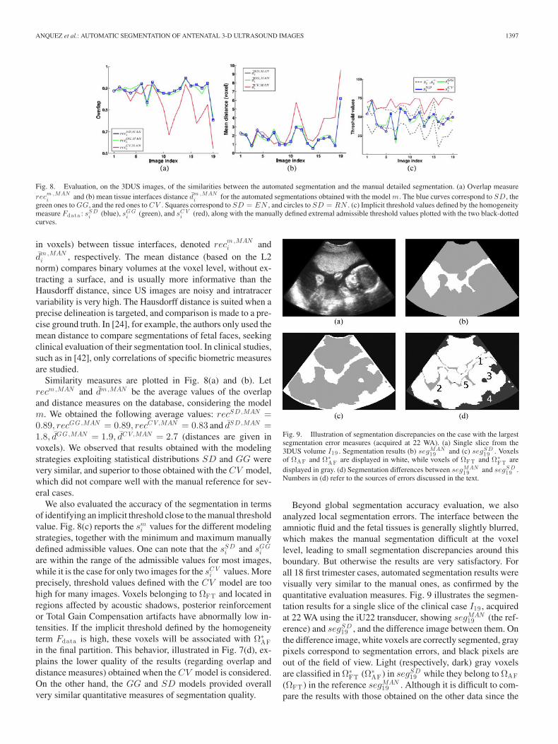
Fig. 8. Evaluation, on the 3DUS images, of the similarities between the automated segmentation and the manual detailed segmentation. (a) Overlap measurerecm ,MAN

i and (b) mean tissue interfaces distance dm ,MANi for the automated segmentations obtained with the model m. The blue curves correspond to SD, the

green ones to GG, and the red ones to CV . Squares correspond to SD = EN , and circles to SD = RN . (c) Implicit threshold values defined by the homogeneitymeasure Fdata : sS D

i (blue), sG Gi (green), and sC V

i (red), along with the manually defined extremal admissible threshold values plotted with the two black-dottedcurves.

in voxels) between tissue interfaces, denoted recm,MANi and

dm ,MANi , respectively. The mean distance (based on the L2

norm) compares binary volumes at the voxel level, without ex-tracting a surface, and is usually more informative than theHausdorff distance, since US images are noisy and intratracervariability is very high. The Hausdorff distance is suited when aprecise delineation is targeted, and comparison is made to a pre-cise ground truth. In [24], for example, the authors only used themean distance to compare segmentations of fetal faces, seekingclinical evaluation of their segmentation tool. In clinical studies,such as in [42], only correlations of specific biometric measuresare studied.

Similarity measures are plotted in Fig. 8(a) and (b). Letrecm,MAN and dm ,MAN be the average values of the overlapand distance measures on the database, considering the modelm. We obtained the following average values: recSD,MAN =0.89, recGG,MAN = 0.89, recC V ,MAN = 0.83 and dSD,MAN =1.8, dGG,MAN = 1.9, dC V ,MAN = 2.7 (distances are given invoxels). We observed that results obtained with the modelingstrategies exploiting statistical distributions SD and GG werevery similar, and superior to those obtained with the CV model,which did not compare well with the manual reference for sev-eral cases.

We also evaluated the accuracy of the segmentation in termsof identifying an implicit threshold close to the manual thresholdvalue. Fig. 8(c) reports the sm

i values for the different modelingstrategies, together with the minimum and maximum manuallydefined admissible values. One can note that the sSD

i and sGGi

are within the range of the admissible values for most images,while it is the case for only two images for the sC V

i values. Moreprecisely, threshold values defined with the CV model are toohigh for many images. Voxels belonging to ΩFT and located inregions affected by acoustic shadows, posterior reinforcementor Total Gain Compensation artifacts have abnormally low in-tensities. If the implicit threshold defined by the homogeneityterm Fdata is high, these voxels will be associated with Ω∗

AFin the final partition. This behavior, illustrated in Fig. 7(d), ex-plains the lower quality of the results (regarding overlap anddistance measures) obtained when the CV model is considered.On the other hand, the GG and SD models provided overallvery similar quantitative measures of segmentation quality.

Fig. 9. Illustration of segmentation discrepancies on the case with the largestsegmentation error measures (acquired at 22 WA). (a) Single slice from the3DUS volume I19 . Segmentation results (b) segMAN

19 and (c) segS D19 . Voxels

of ΩAF and Ω∗AF are displayed in white, while voxels of ΩFT and Ω∗

FT aredisplayed in gray. (d) Segmentation differences between segMAN

19 and segS D19 .

Numbers in (d) refer to the sources of errors discussed in the text.

Beyond global segmentation accuracy evaluation, we alsoanalyzed local segmentation errors. The interface between theamniotic fluid and the fetal tissues is generally slightly blurred,which makes the manual segmentation difficult at the voxellevel, leading to small segmentation discrepancies around thisboundary. But otherwise the results are very satisfactory. Forall 18 first trimester cases, automated segmentation results werevisually very similar to the manual ones, as confirmed by thequantitative evaluation measures. Fig. 9 illustrates the segmen-tation results for a single slice of the clinical case I19 , acquiredat 22 WA using the iU22 transducer, showing segMAN

19 (the ref-erence) and segSD

19 , and the difference image between them. Onthe difference image, white voxels are correctly segmented, graypixels correspond to segmentation errors, and black pixels areout of the field of view. Light (respectively, dark) gray voxelsare classified in Ω∗

FT (Ω∗AF ) in segSD

19 while they belong to ΩAF(ΩFT ) in the reference segMAN

19 . Although it is difficult to com-pare the results with those obtained on the other data since the


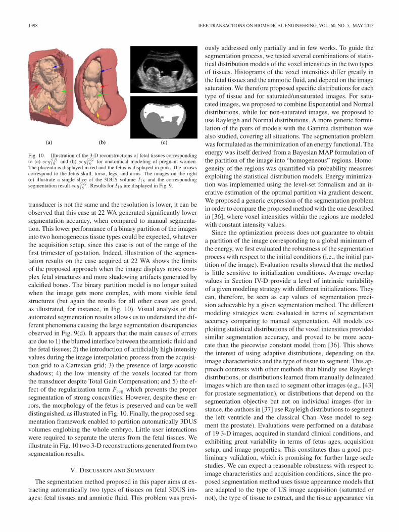
Fig. 10. Illustration of the 3-D reconstructions of fetal tissues correspondingto (a) segS D

19 and (b) segG G18 for anatomical modeling of pregnant women.

The placenta is displayed in red and the fetus is displayed in pink. The arrowscorrespond to the fetus skull, torso, legs, and arms. The images on the right(c) illustrate a single slice of the 3DUS volume I18 and the correspondingsegmentation result segG G

18 . Results for I19 are displayed in Fig. 9.

transducer is not the same and the resolution is lower, it can beobserved that this case at 22 WA generated significantly lowersegmentation accuracy, when compared to manual segmenta-tion. This lower performance of a binary partition of the imagesinto two homogeneous tissue types could be expected, whateverthe acquisition setup, since this case is out of the range of thefirst trimester of gestation. Indeed, illustration of the segmen-tation results on the case acquired at 22 WA shows the limitsof the proposed approach when the image displays more com-plex fetal structures and more shadowing artifacts generated bycalcified bones. The binary partition model is no longer suitedwhen the image gets more complex, with more visible fetalstructures (but again the results for all other cases are good,as illustrated, for instance, in Fig. 10). Visual analysis of theautomated segmentation results allows us to understand the dif-ferent phenomena causing the large segmentation discrepanciesobserved in Fig. 9(d). It appears that the main causes of errorsare due to 1) the blurred interface between the amniotic fluid andthe fetal tissues; 2) the introduction of artificially high intensityvalues during the image interpolation process from the acquisi-tion grid to a Cartesian grid; 3) the presence of large acousticshadows; 4) the low intensity of the voxels located far fromthe transducer despite Total Gain Compensation; and 5) the ef-fect of the regularization term Freg which prevents the propersegmentation of strong concavities. However, despite these er-rors, the morphology of the fetus is preserved and can be welldistinguished, as illustrated in Fig. 10. Finally, the proposed seg-mentation framework enabled to partition automatically 3DUSvolumes englobing the whole embryo. Little user interactionswere required to separate the uterus from the fetal tissues. Weillustrate in Fig. 10 two 3-D reconstructions generated from twosegmentation results.

V. DISCUSSION AND SUMMARY

The segmentation method proposed in this paper aims at ex-tracting automatically two types of tissues on fetal 3DUS im-ages: fetal tissues and amniotic fluid. This problem was previ-

ously addressed only partially and in few works. To guide thesegmentation process, we tested several combinations of statis-tical distribution models of the voxel intensities in the two typesof tissues. Histograms of the voxel intensities differ greatly inthe fetal tissues and the amniotic fluid, and depend on the imagesaturation. We therefore proposed specific distributions for eachtype of tissue and for saturated/unsaturated images. For satu-rated images, we proposed to combine Exponential and Normaldistributions, while for non-saturated images, we proposed touse Rayleigh and Normal distributions. A more generic formu-lation of the pairs of models with the Gamma distribution wasalso studied, covering all situations. The segmentation problemwas formulated as the minimization of an energy functional. Theenergy was itself derived from a Bayesian MAP formulation ofthe partition of the image into “homogeneous” regions. Homo-geneity of the regions was quantified via probability measuresexploiting the statistical distribution models. Energy minimiza-tion was implemented using the level-set formalism and an it-erative estimation of the optimal partition via gradient descent.We proposed a generic expression of the segmentation problemin order to compare the proposed method with the one describedin [36], where voxel intensities within the regions are modeledwith constant intensity values.

Since the optimization process does not guarantee to obtaina partition of the image corresponding to a global minimum ofthe energy, we first evaluated the robustness of the segmentationprocess with respect to the initial conditions (i.e., the initial par-tition of the image). Evaluation results showed that the methodis little sensitive to initialization conditions. Average overlapvalues in Section IV-D provide a level of intrinsic variabilityof a given modeling strategy with different initializations. Theycan, therefore, be seen as cap values of segmentation preci-sion achievable by a given segmentation method. The differentmodeling strategies were evaluated in terms of segmentationaccuracy comparing to manual segmentation. All models ex-ploiting statistical distributions of the voxel intensities providedsimilar segmentation accuracy, and proved to be more accu-rate than the piecewise constant model from [36]. This showsthe interest of using adaptive distributions, depending on theimage characteristics and the type of tissue to segment. This ap-proach contrasts with other methods that blindly use Rayleighdistributions, or distributions learned from manually delineatedimages which are then used to segment other images (e.g., [43]for prostate segmentation), or distributions that depend on thesegmentation objective but not on individual images (for in-stance, the authors in [37] use Rayleigh distributions to segmentthe left ventricle and the classical Chan–Vese model to seg-ment the prostate). Evaluations were performed on a databaseof 19 3-D images, acquired in standard clinical conditions, andexhibiting great variability in terms of fetus ages, acquisitionsetup, and image properties. This constitutes thus a good pre-liminary validation, which is promising for further large-scalestudies. We can expect a reasonable robustness with respect toimage characteristics and acquisition conditions, since the pro-posed segmentation method uses tissue appearance models thatare adapted to the type of US image acquisition (saturated ornot), the type of tissue to extract, and the tissue appearance via


optimization of the modeling parameters, and since segmen-tation performances were stable for 19 cases, acquired inclinical routine and not optimized for this particular study.More extensive clinical validation could be based on severalmanual segmentations, provided by different experts, so thatinter-expert variability could be assessed. A next step could alsobe to provide a methodology to decide a priori on the bestmodeling strategy.

Our segmentation method was implemented in MATLAB,without code optimization. An order of magnitude of 20 minutesfor a 100 × 200 × 100 matrix size was needed for the wholeprocess. The only hint to reduce running time, besides codeoptimization, is to start with a good initialization, hence reducingthe number of iterations.

Three-dimensional reconstructions, based on the segmenta-tion results, were illustrated and enabled to precisely visualizethe fetus in the uterine environment, even on challenging imageswith strong artifacts.

The segmentation results provided by our method were inter-actively refined by distinguishing the fetus body, the umbilicalcord, and the placenta. Since the contact region between thefetus and the uterine wall is small, little user interaction wasrequired to perform this task. In a clinical context, the VOCALsoftware tool can be used to interactively segment the amnioticsac as proposed in [44], with limited effort thanks to the pow-erful visualization and interaction functionalities of this tool.Echographers are getting familiar with the manipulation of suchinteractive segmentation tools for 3DUS images but still con-sider a full segmentation to be cumbersome in clinical routine.Future methodological developments will consist in identifyingthe three aforementioned structures, in an automated or semi-automated fashion, for applications such as biometric measures(amniotic sac and fetal volumes, crown-rump length, etc.) onlarge datasets.

Morphological and biometrical analysis of the fetus could beperformed using the proposed automated segmentation tool.There are several potential clinical applications for the ex-ploitation of detailed segmentations of the fetus during the firsttrimester: detection of asymmetries between the cephalic poleand the embryo’s body is of interest to identify severe abnormali-ties and identify potential correlation with miscarriage probabil-ity; quantification of fetus volumes could be exploited to assessfetal development and refine delivery date prediction; finer im-age markers of abnormalities could be investigated, exploitingthe automated localization of the ocular lobes, the limbs, thestomach, the bladder, and the nuchal translucency; comparisonof 3-D measures with 1-D/2-D measurements extracted fromstandard 2-D echographic images is still needed to evaluate theclinical impact of 3DUS imaging for biometry.

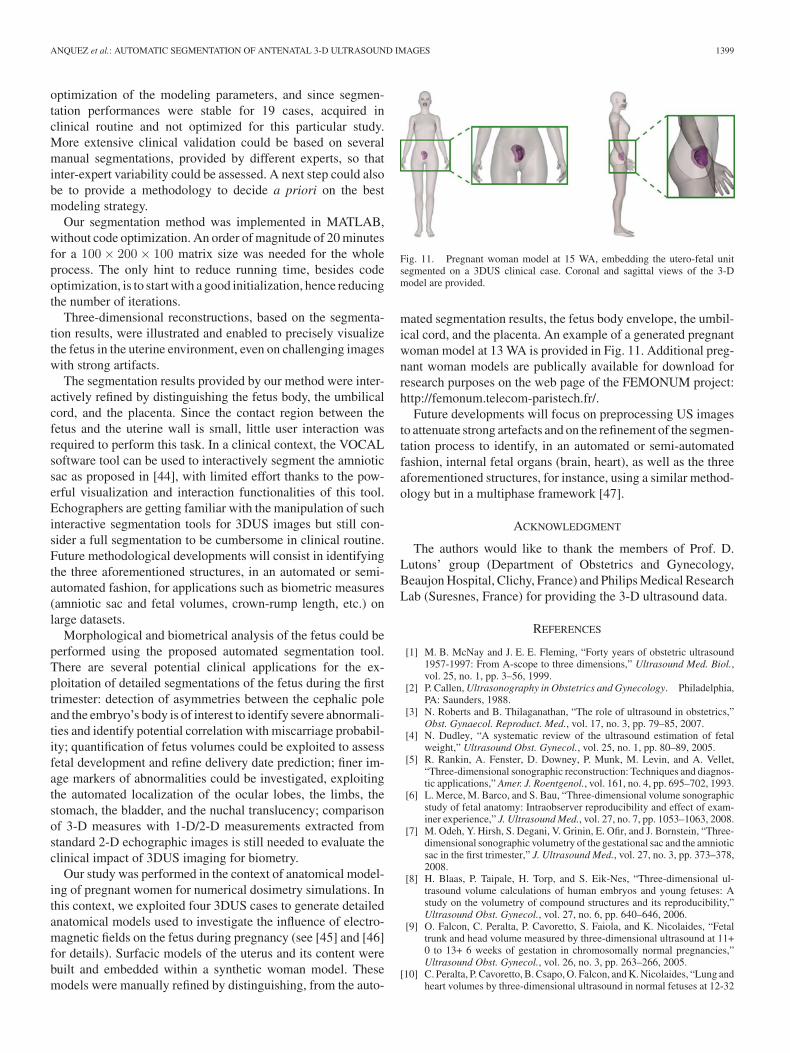
Our study was performed in the context of anatomical model-ing of pregnant women for numerical dosimetry simulations. Inthis context, we exploited four 3DUS cases to generate detailedanatomical models used to investigate the influence of electro-magnetic fields on the fetus during pregnancy (see [45] and [46]for details). Surfacic models of the uterus and its content werebuilt and embedded within a synthetic woman model. Thesemodels were manually refined by distinguishing, from the auto-

Fig. 11. Pregnant woman model at 15 WA, embedding the utero-fetal unitsegmented on a 3DUS clinical case. Coronal and sagittal views of the 3-Dmodel are provided.

mated segmentation results, the fetus body envelope, the umbil-ical cord, and the placenta. An example of a generated pregnantwoman model at 13 WA is provided in Fig. 11. Additional preg-nant woman models are publically available for download forresearch purposes on the web page of the FEMONUM project:http://femonum.telecom-paristech.fr/.

Future developments will focus on preprocessing US imagesto attenuate strong artefacts and on the refinement of the segmen-tation process to identify, in an automated or semi-automatedfashion, internal fetal organs (brain, heart), as well as the threeaforementioned structures, for instance, using a similar method-ology but in a multiphase framework [47].

ACKNOWLEDGMENT

The authors would like to thank the members of Prof. D.Lutons’ group (Department of Obstetrics and Gynecology,Beaujon Hospital, Clichy, France) and Philips Medical ResearchLab (Suresnes, France) for providing the 3-D ultrasound data.

REFERENCES

[1] M. B. McNay and J. E. E. Fleming, “Forty years of obstetric ultrasound1957-1997: From A-scope to three dimensions,” Ultrasound Med. Biol.,vol. 25, no. 1, pp. 3–56, 1999.

[2] P. Callen, Ultrasonography in Obstetrics and Gynecology. Philadelphia,PA: Saunders, 1988.

[3] N. Roberts and B. Thilaganathan, “The role of ultrasound in obstetrics,”Obst. Gynaecol. Reproduct. Med., vol. 17, no. 3, pp. 79–85, 2007.

[4] N. Dudley, “A systematic review of the ultrasound estimation of fetalweight,” Ultrasound Obst. Gynecol., vol. 25, no. 1, pp. 80–89, 2005.

[5] R. Rankin, A. Fenster, D. Downey, P. Munk, M. Levin, and A. Vellet,“Three-dimensional sonographic reconstruction: Techniques and diagnos-tic applications,” Amer. J. Roentgenol., vol. 161, no. 4, pp. 695–702, 1993.

[6] L. Merce, M. Barco, and S. Bau, “Three-dimensional volume sonographicstudy of fetal anatomy: Intraobserver reproducibility and effect of exam-iner experience,” J. Ultrasound Med., vol. 27, no. 7, pp. 1053–1063, 2008.

[7] M. Odeh, Y. Hirsh, S. Degani, V. Grinin, E. Ofir, and J. Bornstein, “Three-dimensional sonographic volumetry of the gestational sac and the amnioticsac in the first trimester,” J. Ultrasound Med., vol. 27, no. 3, pp. 373–378,2008.

[8] H. Blaas, P. Taipale, H. Torp, and S. Eik-Nes, “Three-dimensional ul-trasound volume calculations of human embryos and young fetuses: Astudy on the volumetry of compound structures and its reproducibility,”Ultrasound Obst. Gynecol., vol. 27, no. 6, pp. 640–646, 2006.

[9] O. Falcon, C. Peralta, P. Cavoretto, S. Faiola, and K. Nicolaides, “Fetaltrunk and head volume measured by three-dimensional ultrasound at 11+0 to 13+ 6 weeks of gestation in chromosomally normal pregnancies,”Ultrasound Obst. Gynecol., vol. 26, no. 3, pp. 263–266, 2005.

[10] C. Peralta, P. Cavoretto, B. Csapo, O. Falcon, and K. Nicolaides, “Lung andheart volumes by three-dimensional ultrasound in normal fetuses at 12-32


weeks gestation,” Ultrasound Obst. Gynecol., vol. 27, no. 2, pp. 128–133,2006.

[11] N. Raine-Fenning, J. Clewes, N. Kendall, A. Bunkheila, B. Campbell, andI. Johnson, “The interobserver reliability and validity of volume calcula-tion from three-dimensional ultrasound datasets in the in vitro setting,”Ultrasound Obst. Gynecol., vol. 21, no. 3, pp. 283–291, 2003.

[12] B. Tutschek and D. Sahn, “Semi-automatic segmentation of fetal cardiaccavities: Progress towards an automated fetal echocardiogram,” Ultra-sound Obst. Gynecol., vol. 32, no. 2, pp. 176–180, 2008.

[13] A. Noble and D. Boukerroui, “Ultrasound image segmentation: A survey,”IEEE Trans. Med. Imag., vol. 25, no. 8, pp. 987–1010, Aug. 2006.

[14] J. Thomas, R. Petters, and P. Jeanty, “Automatic segmentation of ultra-sound images using morphological operators,” IEEE Trans. Med. Imag.,vol. 10, no. 2, pp. 180–186, Jun. 1991.

[15] G. Matsopoulos and S. Marshall, “Use of morphological image processingtechniques for the measurement of a fetal head from ultrasound images,”Pattern Recognit., vol. 27, no. 10, pp. 1317–1324, 1994.

[16] M. Kass, A. Witkin, and D. Terzopoulos, “Snakes: Active contour models,”Int. J. Comput. Vis., vol. 1, no. 4, pp. 321–331, 1988.

[17] V. Chalana, T. Winter 3rd, D. Cyr, D. Haynor, and Y. Kim, “Automaticfetal head measurements from sonographic images,” Acad. Radiol., vol. 3,no. 8, pp. 628–635, 1996.

[18] S. Jardim and M. Figueiredo, “Segmentation of fetal ultrasound images,”Ultrasound Med. Biol., vol. 31, no. 2, pp. 243–250, 2005.

[19] G. Carneiro, B. Georgescu, S. Good, and D. Comaniciu, “Detection andmeasurement of fetal anatomies from ultrasound images using a con-strained probabilistic boosting tree,” IEEE Trans. Med. Imag., vol. 27,no. 9, pp. 1342–1355, Sep. 2008.

[20] A. Sarti, R. Malladi, and J. Sethian, “Subjective surfaces: A geometricmodel for boundary completion,” Int. J. Comput. Vis., vol. 46, no. 3,pp. 201–221, 2002.

[21] I. Dindoyal, T. Lambrou, J. Deng, C. Ruff, A. Linney, and A. Todd-Pokropek, “Level set segmentation of the foetal heart,” in FunctionalImaging and Modeling of the Heart Proceedings. New York: Springer-Verlag, 2005, pp. 201–221.

[22] A. Sarti, C. Corsi, E. Mazzini, and C. Lamberti, “Maximum likelihood seg-mentation of ultrasound images with Rayleigh distribution,” IEEE Trans.Ultrason., Ferroelectr., Freq. Control, vol. 52, no. 6, pp. 947–960, Jun.2005.

[23] M. Sofka, J. Zhang, S. Zhou, and D. Comaniciu, “Multiple object detectionby sequential Monte Carlo and hierarchical detection network,” in Proc.IEEE Conf. Comput. Vis. Pattern Recognit., Jun. 2010, pp. 1735–1742.

[24] S. Feng, S. Zhou, S. Good, and D. Comaniciu, “Automatic fetal facedetection from ultrasound volumes via learning 3-D and 2-D information,”in Proc. IEEE Conf. Comput. Vis. Pattern Recognit., Jun. 2009, pp. 2488–2495.

[25] G. Carneiro, F. Amat, B. Georgescu, S. Good, and D. Comaniciu,“Semantic-based indexing of fetal anatomies from 3-D ultrasound datausing global/semi-local context and sequential sampling,” in Proc. IEEEConf. Comput. Vis. Pattern Recognit., Jun. 2008, pp. 1–8.

[26] N. Otsu, “A threshold selection method from gray-level histograms,” Au-tomatica, vol. 11, pp. 285–296, 1975.

[27] J. Hartigan and M. Wong, “A k-means clustering algorithm,” Appl. Statist.,vol. 28, no. 1, pp. 100–108, 1979.

[28] S. Choi and R. Wette, “Maximum likelihood estimation of the parametersof the gamma distribution and their bias,” Technometrics, vol. 11, no. 4,pp. 683–690, 1969.

[29] Z. Tao, H. Tagare, and J. Beaty, “Evaluation of four probability distributionmodels for speckle in clinical cardiac ultrasound images,” IEEE Trans.Med. Imag., vol. 25, no. 11, pp. 1483–1491, Nov. 2006.

[30] R. Wagner, S. Smith, J. Sandrik, and H. Lopez, “Statistics of speckle inultrasound B-scans,” IEEE Trans. Sonics Ultrason., vol. SU-30, no. 3,pp. 156–163, May 1983.

[31] C. Burckhardt, “Speckle in ultrasound B-mode scans,” IEEE Trans. SonicsUltrason., vol. SU-25, no. 1, pp. 1–6, Jan. 1978.

[32] N. Paragios, M. Jolly, M. Taron, and R. Ramaraj, “Active shape modelsand segmentation of the left ventricle in echocardiography,” in Proceed-ings of the International Conference on Scale Space Theories PDEs Meth-ods Computer Vision. New York: Springer-Verlag, 2005, pp. 131–142.

[33] M. Hansen, J. Moller, and F. Togersen, “Bayesian contour detection in atime series of ultrasound images through dynamic deformable templatemodels,” Biostatistics, vol. 3, no. 2, pp. 213–228, 2002.

[34] F. Shao, K. Ling, and W. Ng, “Automatic 3-D prostate surface detectionfrom TRUS with level sets,” Int. J. Imag. Graph., vol. 4, no. 3, pp. 385–403, 2004.

[35] J. Durbin and M. Knott, “Components of Cramer-von Mises statistics. I,”J. Royal Statist. Soc. Ser. B, vol. 34, pp. 290–307, 1972.

[36] T. Chan and L. Vese, “Active contours without edges,” IEEE Trans. Imag.Process., vol. 10, no. 2, pp. 266–277, Feb. 2001.

[37] C. Ahn, Y. Jung, O. Kwon, and J. Seo, “A regularization technique forclosed contour segmentation in ultrasound images,” IEEE Trans. Ultra-son., Ferroelectr., Freq. Control, vol. 58, no. 8, pp. 1577–1589, Aug. 2011.

[38] S. Osher and J. Sethian, Fronts Propagating With Curvature DependentSpeed: Algorithms Based on Hamilton-Jacobi Formulations. Hampton,VA: NASA Langley Res. Center, 1987.

[39] S. Osher and N. Paragios, Geometric Level Set Methods in Imaging, Vision,and Graphics. New York: Springer-Verlag, 2003.

[40] M. Rousson and R. Deriche, “A variational framework for active andadaptive segmentation of vector valued images,” in Proc. IEEE WorkshopMotion Video Comput., Dec. 2002, pp. 56–62.

[41] L. Vese and T. Chan, “A multiphase level set framework for image seg-mentation using the Mumford and Shah model,” Int. J. Comput. Vis.,vol. 50, no. 3, pp. 271–293, 2002.

[42] P.-Y. Tsai, H.-C. Chen, H.-H. Huang, C.-H. Chang, P.-S. Fan, C.-I. Huang,Y.-C. Cheng, F.-M. Chang, and Y.-N. Sun, “A new automatic algorithm toextract craniofacial measurements from fetal three-dimensional volumes,”Ultrasound Obst. Gynecol., vol. 39, pp. 642–647, 2012.

[43] R. Xu, O. Michailovich, and M. Salama, “Information tracking approachto segmentation of ultrasound imagery of the prostate,” IEEE Trans. Ul-trason., Ferroelectr., Freq. Control, vol. 57, no. 8, pp. 1748–1761, Aug.2010.

[44] W. Lee, R. Deter, B. McNie, M. Powell, M. Balasubramaniam,L. Goncalves, J. Espinoza, and R. Romero, “Quantitative and morpho-logical assessment of early gestational sacs using three-dimensional ul-trasonography,” Ultrasound Obst. Gynecol., vol. 28, no. 3, pp. 255–260,2006.

[45] J. Anquez, T. Boubekeur, L. Bibin, E. D. Angelini, and I. Bloch, “Utero-fetal unit and pregnant woman modeling using a computer graph-ics approach for dosimetry studies,” in Proc. Med. Image Comput.Comput.-Assisted Intervention, London, U.K., Sep. 2009, vol. LNCS-5761, pp. 1025–1032.

[46] L. Bibin, J. Anquez, J. P. De La Plata Alcalde, T. Boubekeur, E. D. An-gelini, and I. Bloch, “Whole body pregnant woman modeling by digitalgeometry processing with detailed utero-fetal unit based on medical im-ages,” IEEE Trans. Biomed. Eng., vol. 57, no. 10, pp. 2346–2358, Oct.2010.

[47] L. Vese and T. Chan, “A multiphase level set framework for image seg-mentation using the Mumford and Shah model,” Int. J. Comput. Vis.,vol. 50, pp. 271–293, 2002.

Authors’ photographs and biographies not available at the time of publication.

Documents

1388 IEEE TRANSACTIONS ON BIOMEDICAL ENGINEERING, … · family of 2-D methods proposes to segment speciﬁc anatomi-cal structures with morphological operators, ... detailed manual