Embed Size (px)
Citation preview

§1.4 Algorithms and complexity
For a given (optimization) problem,
Questions: 1) how hard is the problem.
2) does there exist an efficient solution algorithm?
Computational complexity analysis (a worst case analysis)
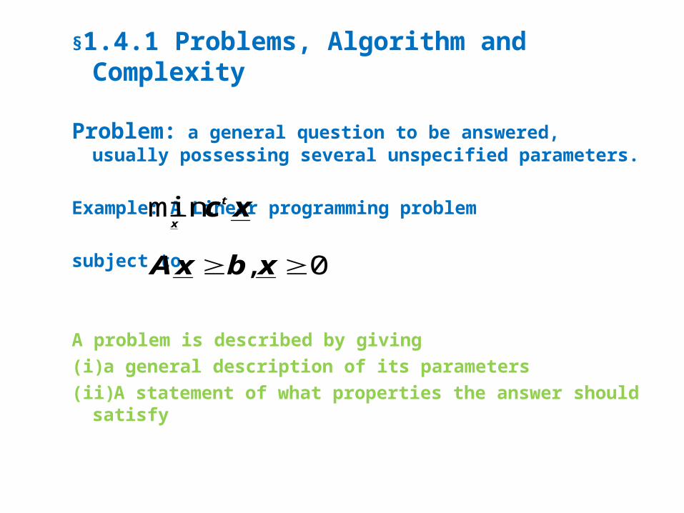
§1.4.1 Problems, Algorithm and Complexity
Problem: a general question to be answered, usually possessing several unspecified parameters.
Example: A Linear programming problem subject to
A problem is described by giving (i) a general description of its parameters(ii)A statement of what properties the answer should satisfy
xc t
xmin
0, xbxA
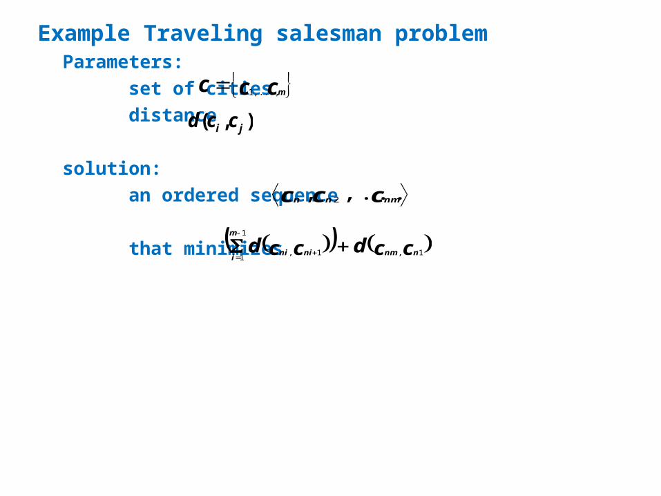
Example Traveling salesman problemParameters:
set of citiesdistance
solution: an ordered sequence
that minimizes
ccc m,...,1
ccc nmnn ,..., 2
ccdccd nnmnini
m
i1,1,
1
1
),( ji ccd
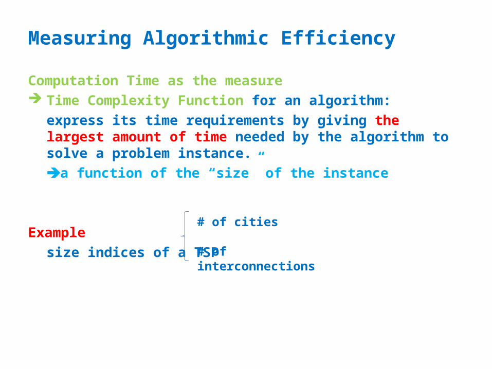
Measuring Algorithmic Efficiency
Computation Time as the measure Time Complexity Function for an algorithm:
express its time requirements by giving the largest amount of time needed by the algorithm to solve a problem instance.a function of the “size” of the instance
Examplesize indices of a TSP
# of cities
# of interconnections
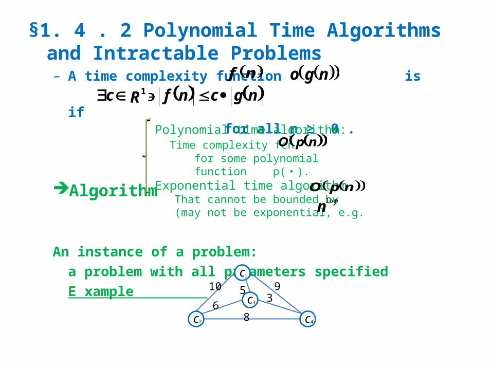
§1. 4 . 2 Polynomial Time Algorithms and Intractable Problems– A time complexity function is
if for all n ≥ 0 .
Algorithm
An instance of a problem:a problem with all parameters specifiedE xample
nf ngo ngcnfRc 1
Polynomial time algorithm: Time complexity fcn. for some polynomial function p( ・ ).Exponential time algorithm That cannot be bounded by (may not be exponential, e.g.
npO
npO
nnlog
c1
c2
c3
c4
5
68
3910
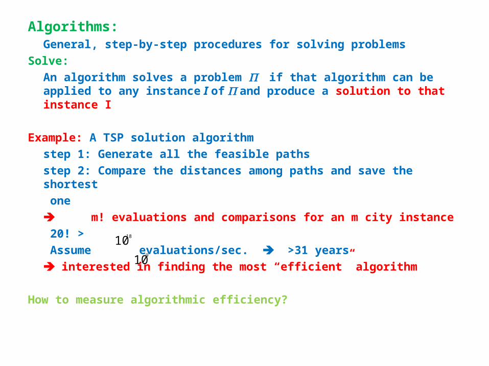
Algorithms:General, step-by-step procedures for solving problems
Solve: An algorithm solves a problem if that algorithm can be applied to any instance I of and produce a solution to that instance I
Example: A TSP solution algorithmstep 1: Generate all the feasible pathsstep 2: Compare the distances among paths and save the shortest
one m! evaluations and comparisons for an m city instance
20! > Assume evaluations/sec. >31 years
interested in finding the most “efficient” algorithm
How to measure algorithmic efficiency?
1018
109
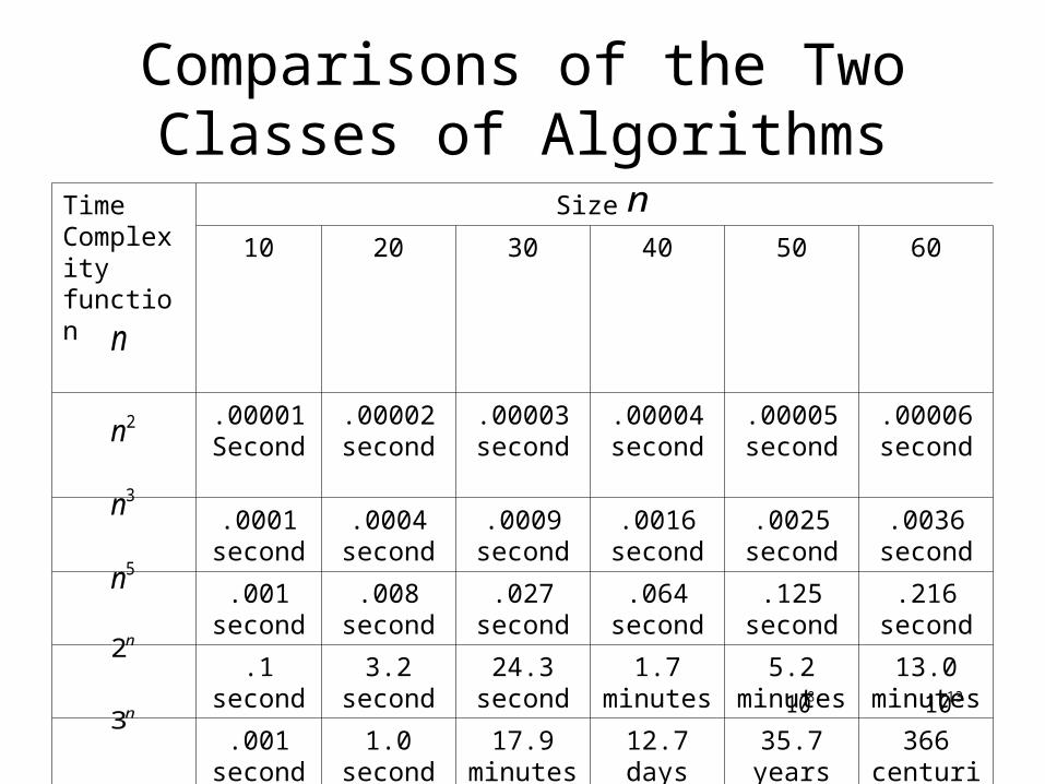
Comparisons of the Two Classes of Algorithms
Time Complexityfunction
Size
10 20 30 40 50 60
.00001Second
.00002second
.00003second
.00004second
.00005second
.00006second
.0001second
.0004second
.0009second
.0016second
.0025second
.0036second
.001second
.008second
.027second
.064second
.125second
.216second
.1second
3.2second
24.3second
1.7minutes
5.2minutes
13.0minutes
.001second
1.0second
17.9minutes
12.7days
35.7years
366centuries
.059second
58minutes
6.5years
3855centuries
2x centuries
1.3x centuries
810 1310
n
2n
3n
n
5n
n2
n3

Size of Largest Problem Instance Solvable in 1 Hour
TimeComplexityfunction
With present Computer
With computer 100 times faster
With computer 1000 times faster
100 1000
10 31.6
4.64 10
2.5 3.98
+6.64 +9.97
+4.19 +6.29
n
2n3n
5n
n2n3
3n
2N
3N
4N
5N
6N
1N
2N
3N
4N
5N
6N
1N
2N
3N
4N
5N
6N
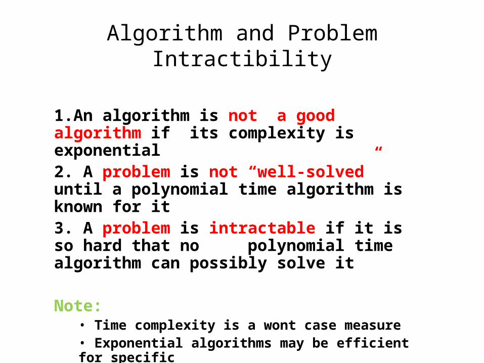
1.An algorithm is not a good algorithm if its complexity is exponential2. A problem is not “well-solved” until a polynomial time algorithm is known for it3. A problem is intractable if it is so hard that no polynomial time algorithm can possibly solve it
Note:• Time complexity is a wont case measure • Exponential algorithms may be efficient for specific applications
Algorithm and Problem Intractibility
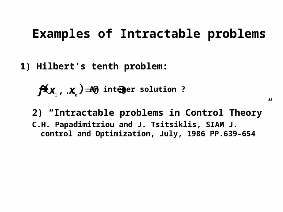
Examples of Intractable problems
1) Hilbert’s tenth problem:
An integer solution ?
2) “Intractable problems in Control Theory”C.H. Papadimitriou and J. Tsitsiklis, SIAM J. control and Optimization,
July, 1986 PP.639-654
0,...1
nxxf

§1.4.4 P and NP Problem, NP-Completeness
• deterministic algorithmsthe result of every operation is uniquely defined e.g. computer programs
• non-deterministic algorithms Results of operations can be any of a set of alternatives
Example: Shopping listA shopping list can be viewed as a very simple nondeterministic algorithm.
Every item on the list is a directive to find the indicated product, but the order in which to find them is not indicated.
• P-class of problems:
the set of all problems which can be solved by deterministic algorithms in polynomial time
• NP-Class of problemsthe set of all problems which can be solved by non-deterministic algorithms in polynomial time
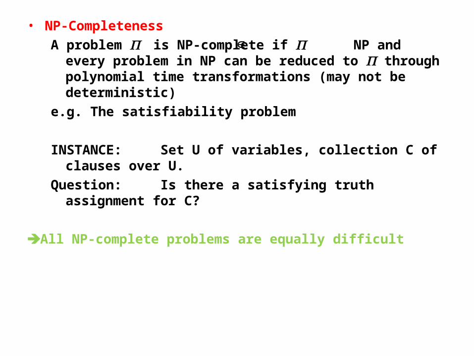
• NP-CompletenessA problem is NP-complete if NP and every problem in NP can
be reduced to through polynomial time transformations (may not be deterministic)
e.g. The satisfiability problem
INSTANCE: Set U of variables, collection C of clauses over U.Question: Is there a satisfying truth assignment for C?
All NP-complete problems are equally difficult
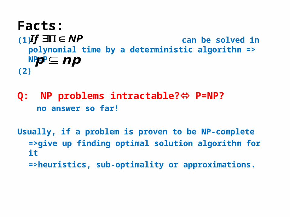
Facts: (1) can be solved in polynomial time by a deterministic
algorithm => NP=P(2)
Q: NP problems intractable? P=NP? no answer so far!
Usually, if a problem is proven to be NP-complete =>give up finding optimal solution algorithm for it=>heuristics, sub-optimality or approximations.
NPIf
npp
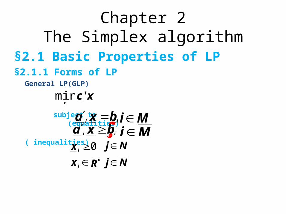
Chapter 2The Simplex algorithm
§2.1 Basic Properties of LP§2.1.1 Forms of LP
General LP(GLP)
subject to (equalities) ( inequalities)
xmin
xc'
ii bxa MiMiii bxa
Rx
xn
j
j
0
Nj
Nj
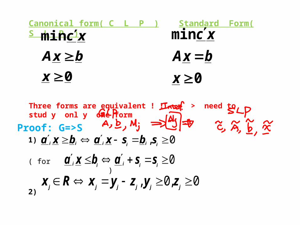
Proof: G=>S1)
( for )
2)
0, iiiiii sbsxabxa
0iiiii ssabxa
0,0, jjjjjjzyzyxRx
Canonical form( C L P ) Standard Form( S L P )
Three forms are equivalent ! ! = > need to stud y onl y one form
0
min
x
bxA
xc
0
min
x
bxA
xc
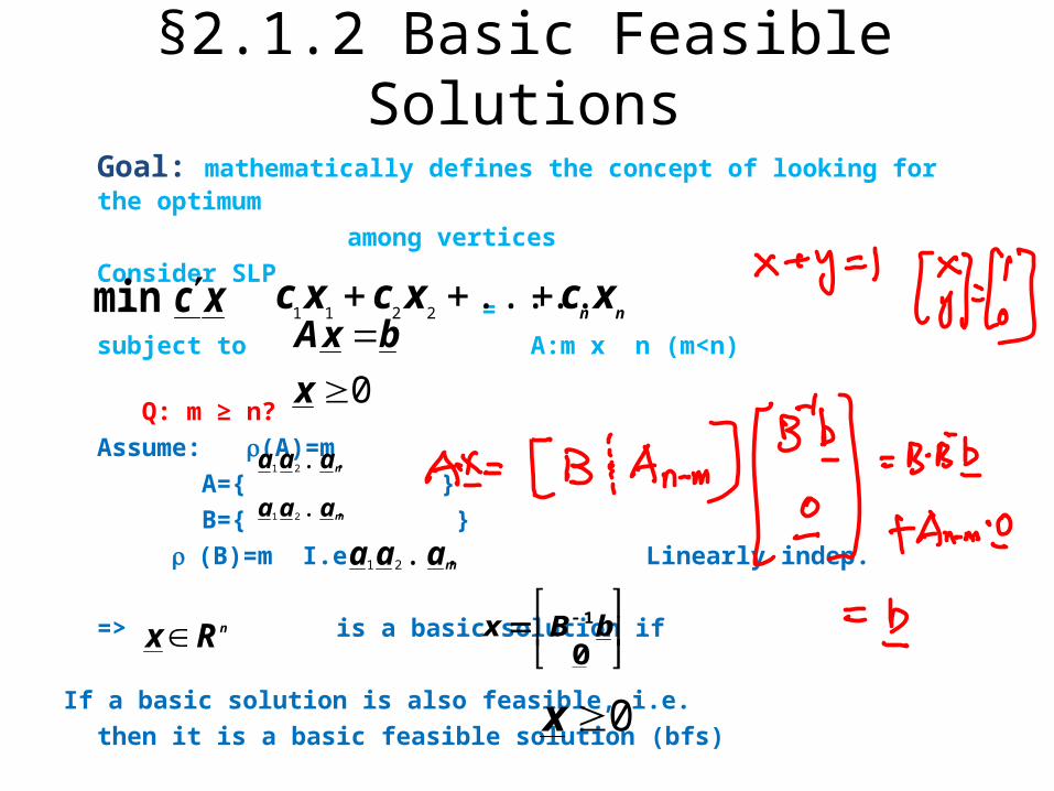
§2.1.2 Basic Feasible Solutions
Goal: mathematically defines the concept of looking for the optimum
among verticesConsider SLP
=subject to A:m x n (m<n)
Q: m ≥ n?Assume: (A)=m
A={ } B={ }
(B)=m I.e. Linearly indep.
=> is a basic solution if If a basic solution is also feasible, i.e.
then it is a basic feasible solution (bfs)
xc min
0
x
bxAnnxcxcxc .....
2211
naaa ...21
maaa ...21
maaa ...21
nRx
0
1bBx
0x
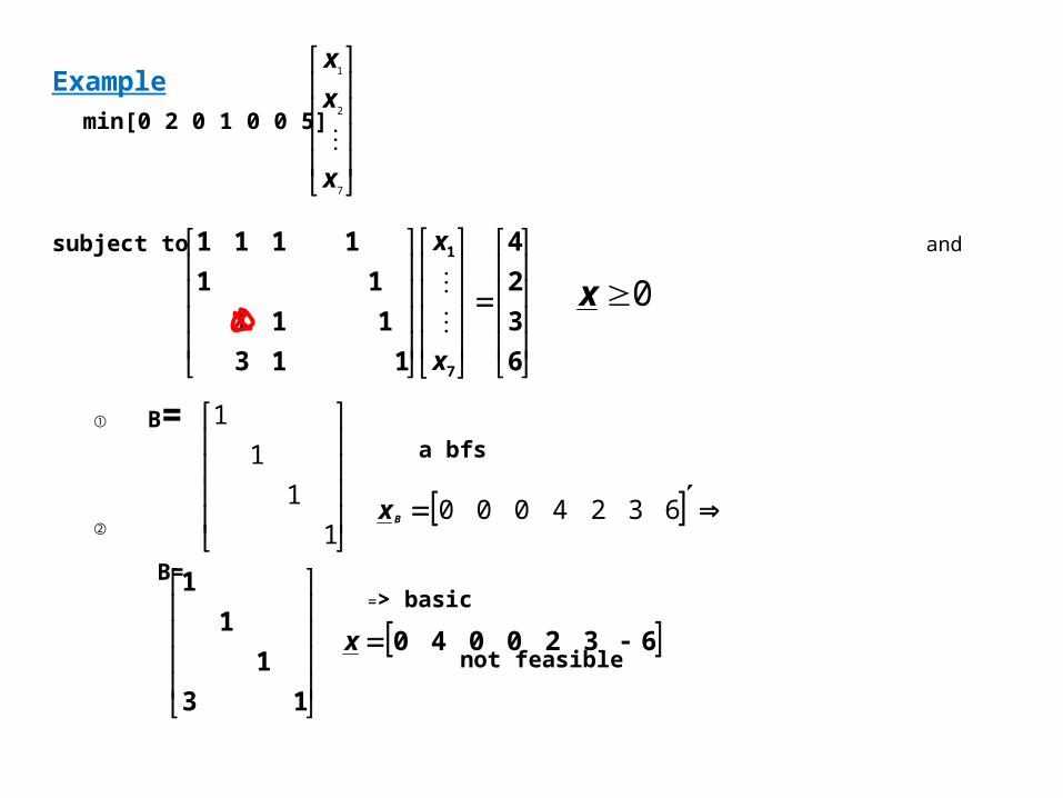
Examplemin[0 2 0 1 0 0 5]
subject to and
① B= a bfs
② B=
= > basic not feasible
7
2
1
x
x
x
6
3
2
4
1 13
1 11
1 1
1111
7
1
x
x
0x
1
1
1
1
6324000Bx
6320040
13
1
1
1
x
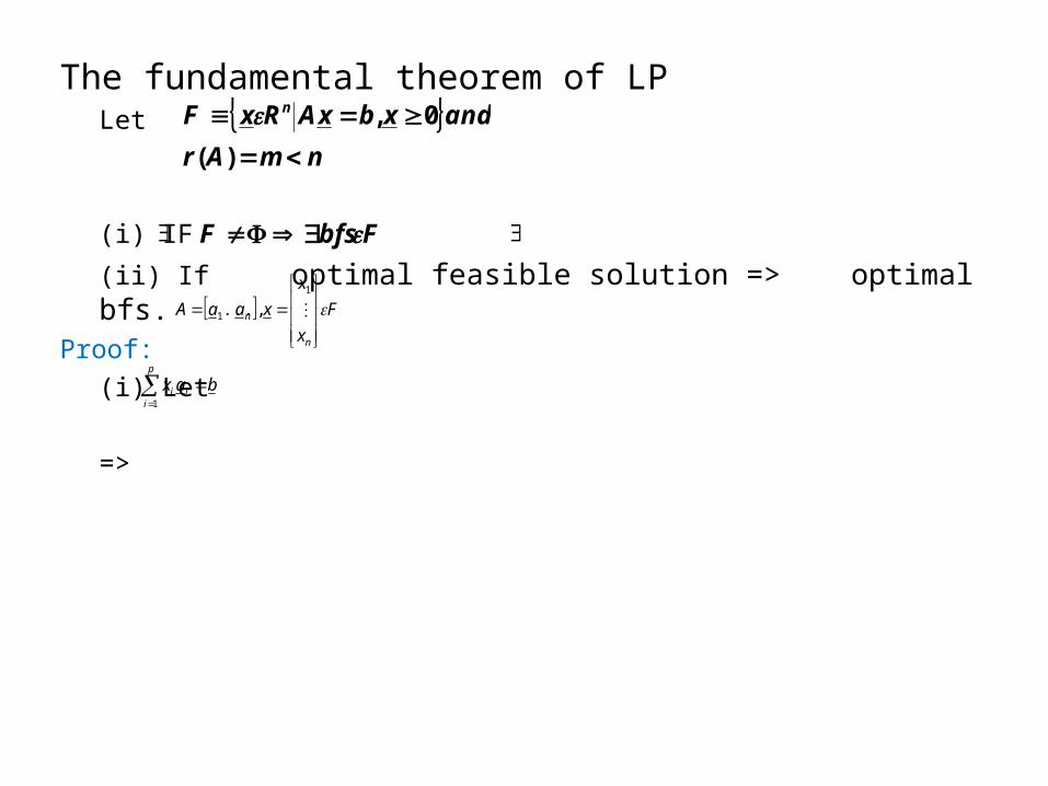
The fundamental theorem of LPLet
(i) IF
(ii) If optimal feasible solution => optimal bfs.Proof:
(i) Let =>
nmAr
andxbxARxF n
)(
0,
FbfsF
F
x
x
xaaA
n
n
1
1 ,...
baxp
iii
1
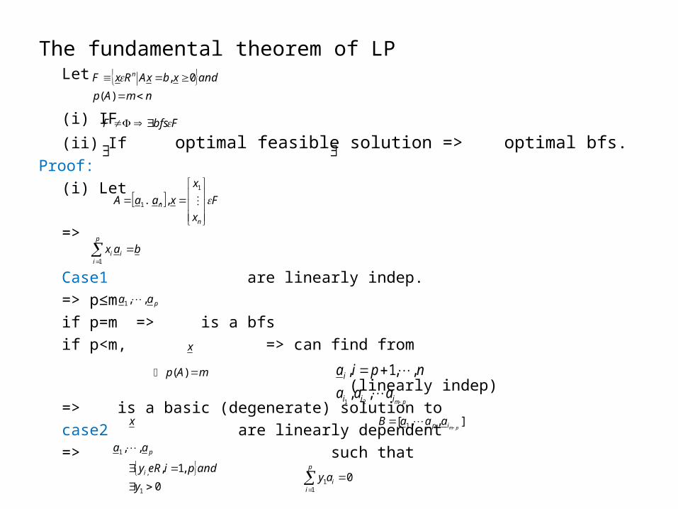
The fundamental theorem of LPLet
(i) IF
(ii) If optimal feasible solution => optimal bfs.Proof:
(i) Let =>
Case1 are linearly indep.=> p≤mif p=m => is a bfs if p<m, => can find from
(linearly indep)=> is a basic (degenerate) solution to
case2 are linearly dependent=> such that
nmAp
andxbxARxF n
)(
0,
FbfsF
F
x
x
xaaA
n
n
1
1 ,...
baxp
iii
1
paa ,,1
x
mAp )(
pmiii
i
aaa
npia
,,
,,1,
21
x ],,[ 1 pmip aaaB
paa ,,1
0
,1,
1
,
y
andpieRyi 01
1
i
p
i
ay
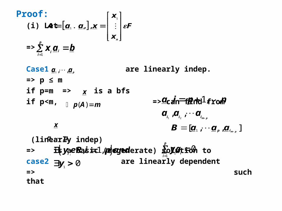
Proof: (i) Let =>
Case1 are linearly indep.=> p ≤ mif p=m => is a bfs if p<m, => can find from
(linearly indep)=> is a basic (degenerate) solution to
case2 are linearly dependent=> such that
F
x
x
xaaA
n
n
1
1 ,...
baxp
iii
1
paa ,,1
x
mAp )(
pmiii
i
aaa
npia
,,
,,1,
21
x ],,[ 1 pmip aaaB
paa ,,1
0
,1,
1
,
y
andpieRyi
01
1
i
p
i
ay
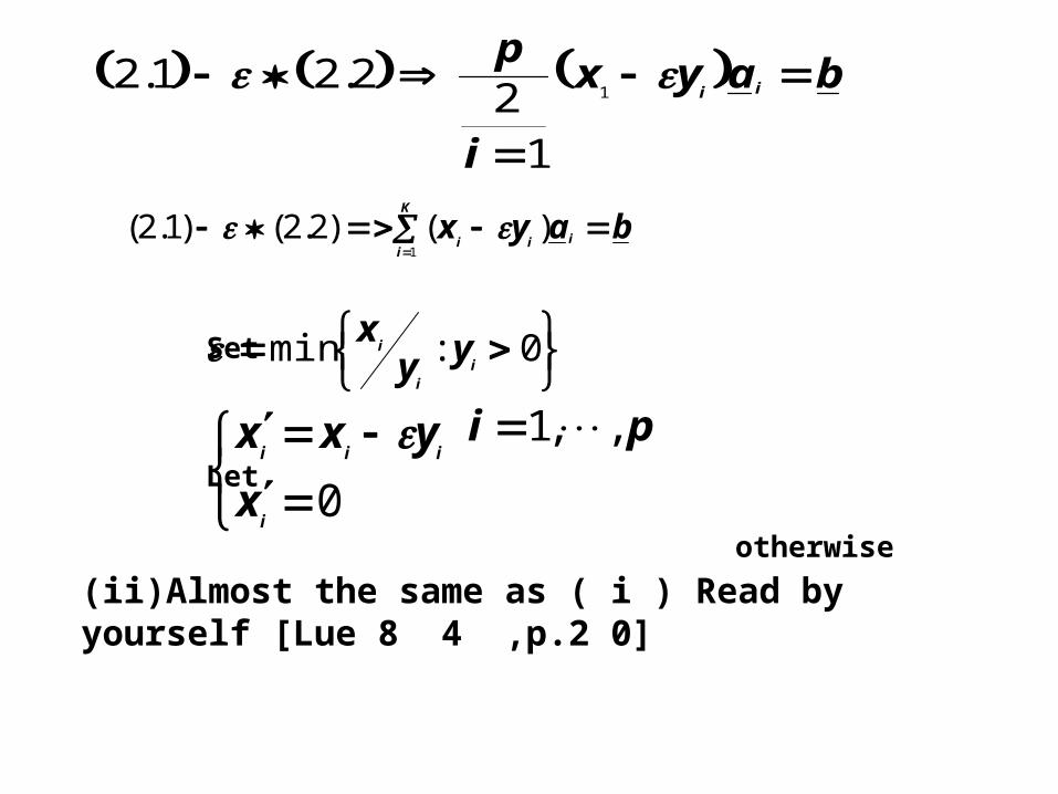
Set
Let otherwise
bayx
i
pii
1
12
2.21.2
bayx ii
K
ii
)()2.2()1.2(1
0:min
ii
i yyx
0i
iii
x
yxx pi ,,1
(ii)Almost the same as ( i ) Read by yourself [Lue 8 4 ,p.2 0]
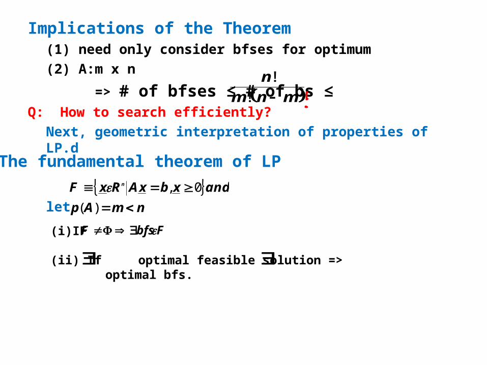
Implications of the Theorem(1) need only consider bfses for optimum(2) A:m x n
=> # of bfses ≤ # of bs ≤ Q: How to search efficiently?
Next, geometric interpretation of properties of LP.d
let
mnm
n
!
!
The fundamental theorem of LP
nmAp
andxbxARxF n
)(
0,
(i) IF
(ii) If optimal feasible solution => optimal bfs.
FbfsF
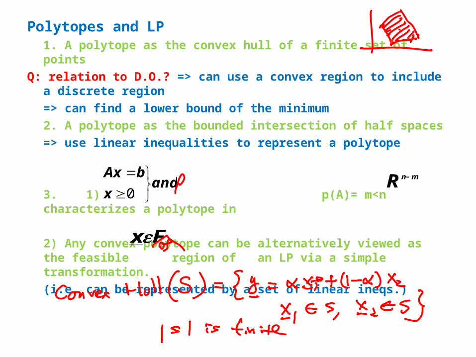
Polytopes and LP1. A polytope as the convex hull of a finite set of points
Q: relation to D.O.? => can use a convex region to include a discrete region=> can find a lower bound of the minimum
2. A polytope as the bounded intersection of half spaces=> use linear inequalities to represent a polytope
3. 1) p(A)= m<n characterizes a polytope in
2) Any convex polytope can be alternatively viewed as the feasible region of an LP via a simple transformation.
(i.e. can be represented by a set of linear ineqs.)
andx
bAx
0
mnR
Fx
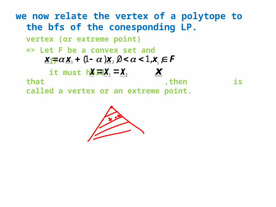
we now relate the vertex of a polytope to the bfs of the conesponding LP.vertex (or extreme point)=> Let F be a convex set and IF it must hold that ,then is called a vertex or an extreme point.
Fxxxx ,,10,)1(121
21 xxx x
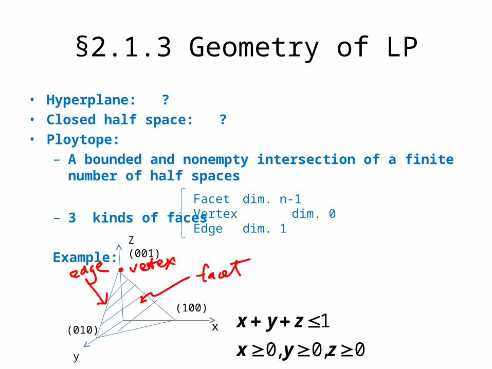
§2.1.3 Geometry of LP
• Hyperplane: ?• Closed half space: ?• Ploytope:
– A bounded and nonempty intersection of a finite number of half spaces
– 3 kinds of faces
Example:
Facet dim. n-1Vertex dim. 0Edge dim. 1
Z(001)
(010) y
x
(100)
0,0,0
1
zyx
zyx
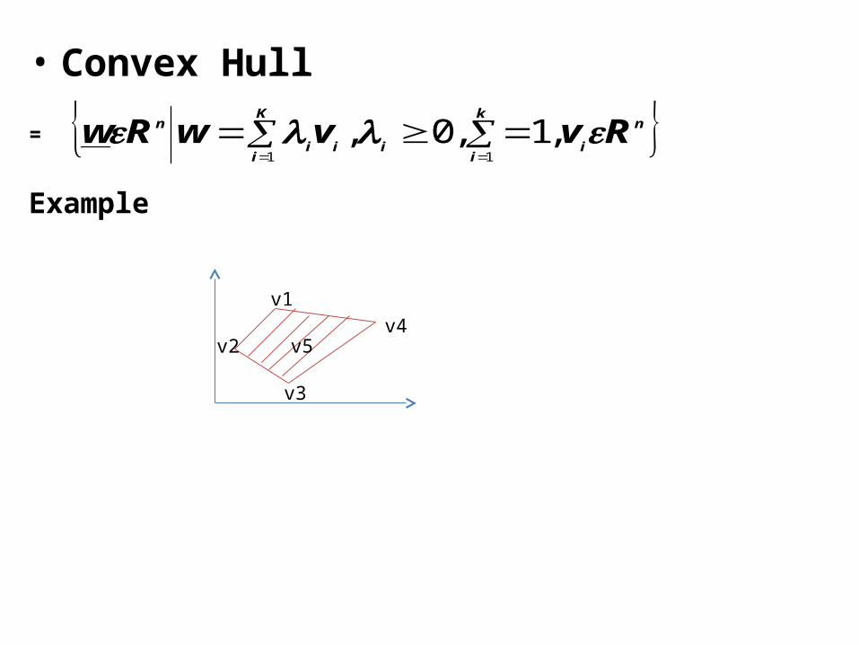
• Convex Hull
=
Example
K
i
k
i
n
iiii
n RvvwRw1 1
,1,0,
v1
v2
v3
v4v5
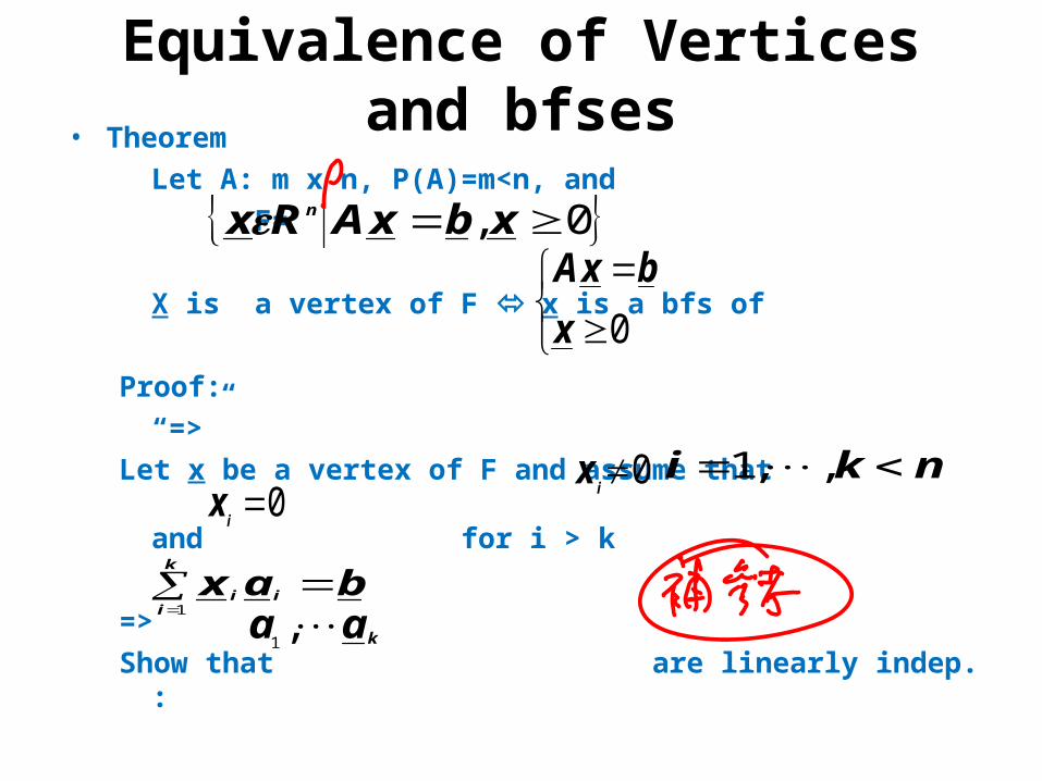
Equivalence of Vertices and bfses• Theorem
Let A: m x n, P(A)=m<n, and F=
X is a vertex of F x is a bfs of
Proof:“=>”
Let x be a vertex of F and assume that and for i > k
=> Show that are linearly indep. :
0, xbxARx n
0x
bxA
0ix nki ,,1
0ix
bax i
k
ii
1
kaa ,1
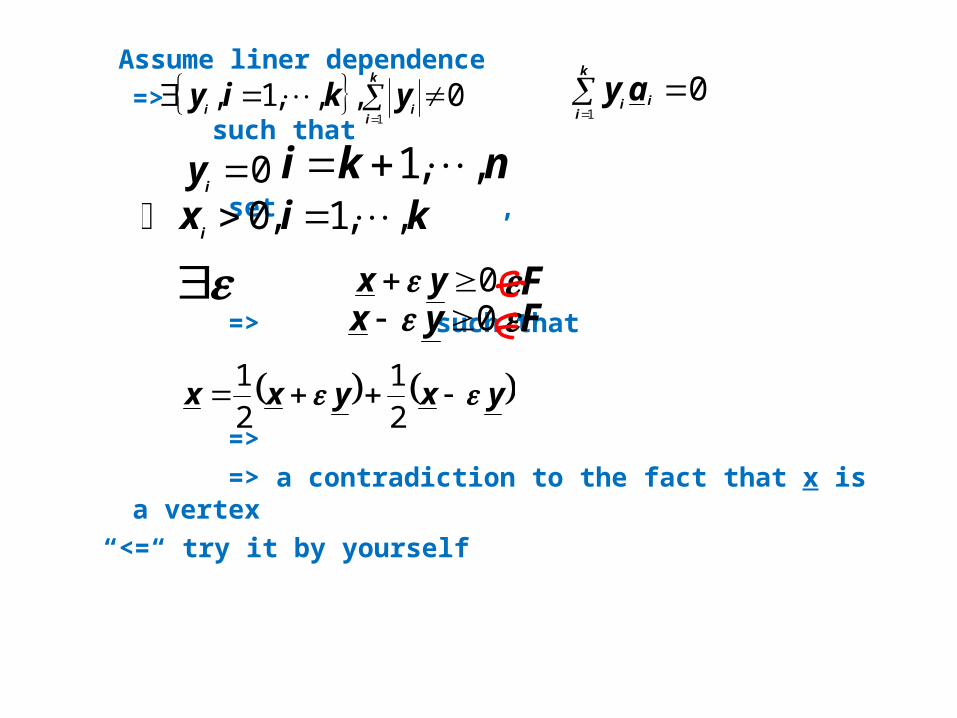
Assume liner dependence=> such that
set ,
=> such that
=>=> a contradiction to the fact that x is a vertex
“<=“ try it by yourself
k
iiiykiy
1
0,,,1, 01
i
k
iiay
0iy nki ,,1
kixi
,,1,0
0 yx F0 yx F
yxyxx 2
1
2
1

§2.2 The Revised Simplex MethodThe simplex method for LP : G.B. Dantzig 1951Key idea:
Phase1:find a bfs of
Note that an LP may not have a solution
Example min s.t.
0x
bxA
21 xx
0,
42
21
21
xx
xx
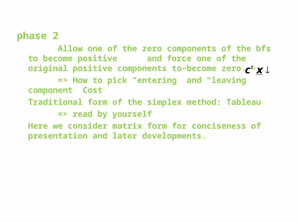
phase 2Allow one of the zero components of the bfs to become positive and force one of the original positive components to become
zero.=> How to pick “entering” and “leaving” component Cost
Traditional form of the simplex method: Tableau=> read by yourself
Here we consider matrix form for conciseness of presentation and later developments.
xcT
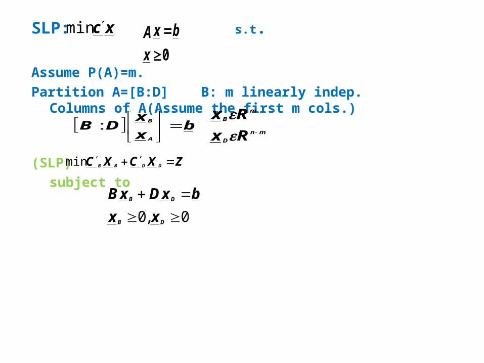
SLP: s.t.
Assume P(A)=m.Partition A=[B:D] B: m linearly indep. Columns of A(Assume the first m
cols.)
(SLP) subject to
xcmin
0
x
bxA
bx
xDB
A
B
:
mn
D
m
B
Rx
Rx
ZXCXC DDBB min
0,0
DB
DB
xx
bxDxB
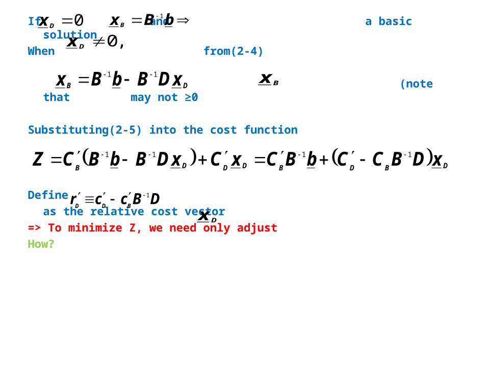
If and a basic solutionWhen from(2-4)
(note that may not ≥0
Substituting(2-5) into the cost function
Define as the relative cost vector
=> To minimize Z, we need only adjust How?
0Dx bBx B
1
,0Dx
BxDB xDBbBx 11
DBDBDDDBxDBCCbBCxCxDBbBCZ 1111
DBccrBDD
1Dx


![Complexity Analysis of Problem-Dimension Using PSO · Complexity Analysis of Problem-Dimension Using PSO ... optimization problems are studied in depth [7]. It ... complexity of problem](https://img.pdfslide.net/doc/110x75/5b0b93567f8b9a99488e1b64/complexity-analysis-of-problem-dimension-using-analysis-of-problem-dimension-using.jpg)