Embed Size (px)
Citation preview
14. Logistic Regression and Newton’s Method
36-402, Advanced Data Analysis
15 March 2011
Reading: Faraway, Chapter 2, omitting sections 2.11 and 2.12
Contents
1 Modeling Conditional Probabilities 1
2 Logistic Regression 32.1 Likelihood Function for Logistic Regression . . . . . . . . . . . . 62.2 Logistic Regression with More Than Two Classes . . . . . . . . . 6
3 Newton’s Method for Numerical Optimization 73.1 Newton’s Method in More than One Dimension . . . . . . . . . . 93.2 Iteratively Re-Weighted Least Squares . . . . . . . . . . . . . . . 10
4 Generalized Linear Models and Generalized Additive Models 114.1 Generalized Additive Models . . . . . . . . . . . . . . . . . . . . 124.2 An Example (Including Model Checking) . . . . . . . . . . . . . 12
1 Modeling Conditional Probabilities
So far, we either looked at estimating the conditional expectations of continuousvariables (as in regression), or at estimating distributions. There are manysituations where however we are interested in input-output relationships, asin regression, but the output variable is discrete rather than continuous. Inparticular there are many situations where we have binary outcomes (it snowsin Pittsburgh on a given day, or it doesn’t; this squirrel carries plague, or itdoesn’t; this loan will be paid back, or it won’t; this person will get heart diseasein the next five years, or they won’t). In addition to the binary outcome, wehave some input variables, which may or may not be continuous. How could wemodel and analyze such data?
We could try to come up with a rule which guesses the binary output fromthe input variables. This is called classification, and is an important topicin statistics and machine learning. However, simply guessing “yes” or “no” ispretty crude — especially if there is no perfect rule. (Why should there be?)
1
Something which takes noise into account, and doesn’t just give a binary answer,will often be useful. In short, we want probabilities — which means we need tofit a stochastic model.
What would be nice, in fact, would be to have conditional distribution ofthe response Y , given the input variables, Pr (Y |X). This would tell us abouthow precise our predictions are. If our model says that there’s a 51% chanceof snow and it doesn’t snow, that’s better than if it had said there was a 99%chance of snow (though even a 99% chance is not a sure thing). We have seenhow to estimate conditional probabilities non-parametrically, and could do thisusing the kernels for discrete variables from lecture 6. While there are a lot ofmerits to this approach, it does involve coming up with a model for the jointdistribution of outputs Y and inputs X, which can be quite time-consuming.
Let’s pick one of the classes and call it “1” and the other “0”. (It doesn’tmatter which is which. Then Y becomes an indicator variable, and youcan convince yourself that Pr (Y = 1) = E [Y ]. Similarly, Pr (Y = 1|X = x) =E [Y |X = x]. (In a phrase, “conditional probability is the conditional expecta-tion of the indicator”.) This helps us because by this point we know all aboutestimating conditional expectations. The most straightforward thing for us todo at this point would be to pick out our favorite smoother and estimate theregression function for the indicator variable; this will be an estimate of theconditional probability function.
There are two reasons not to just plunge ahead with that idea. One is thatprobabilities must be between 0 and 1, but our smoothers will not necessarilyrespect that, even if all the observed yi they get are either 0 or 1. The other isthat we might be better off making more use of the fact that we are trying toestimate probabilities, by more explicitly modeling the probability.
Assume that Pr (Y = 1|X = x) = p(x; θ), for some function p parameter-ized by θ. parameterized function θ, and further assume that observations areindependent of each other. The the (conditional) likelihood function is
n∏i=1
Pr (Y = yi|X = xi) =n∏i=1
p(xi; θ)yi(1− p(xi; θ)1−yi)
Recall that in a sequence of Bernoulli trials y1, . . . yn, where there is a con-stant probability of success p, the likelihood is
n∏i=1
pyi(1− p)1−yi
As you learned in intro. stats, this likelihood is maximized when p = p̂ =n−1
∑ni=1 yi. If each trial had its own success probability pi, this likelihood
becomesn∏i=1
pyi
i (1− pi)1−yi
Without some constraints, estimating the “inhomogeneous Bernoulli” model bymaximum likelihood doesn’t work; we’d get p̂i = 1 when yi = 1, p̂i = 0 when
2
yi = 0, and learn nothing. If on the other hand we assume that the pi aren’tjust arbitrary numbers but are linked together, those constraints give non-trivialparameter estimates, and let us generalize. In the kind of model we are talkingabout, the constraint, pi = p(xi; θ), tells us that pi must be the same wheneverxi is the same, and if p is a continuous function, then similar values of ximust lead to similar values of pi. Assuming p is known (up to parameters), thelikelihood is a function of θ, and we can estimate θ by maximizing the likelihood.This lecture will be about this approach.
2 Logistic Regression
To sum up: we have a binary output variable Y , and we want to model theconditional probability Pr (Y = 1|X = x) as a function of x; any unknown pa-rameters in the function are to be estimated by maximum likelihood. By now,it will not surprise you to learn that statisticians have approach this problemby asking themselves “how can we use linear regression to solve this?”
1. The most obvious idea is to let p(x) be a linear function of x. Everyincrement of a component of x would add or subtract so much to theprobability. The conceptual problem here is that p must be between 0and 1, and linear functions are unbounded.
2. The next most obvious idea is to let log p(x) be a linear function of x,so that changing an input variable multiplies the probability by a fixedamount. The problem is that logarithms are unbounded in only one di-rection, and linear functions are not.
3. Finally, the easiest modification of log p which has an unbounded rangeis the logistic (or logit) transformation, log p
1−p . We can make thisa linear function of x without fear of nonsensical results. (Of course theresults could still happen to be wrong, but they’re not guaranteed to bewrong.)
This last alternative is logistic regression.Formally, the model logistic regression model is that
logp(x)
1− p(x)= β0 + x · β (1)
Solving for p, this gives
p(x; b, w) =eβ0+x·β
1 + eβ0+x·β=
11 + e−(β0+x·β)
(2)
Notice that the over-all specification is a lot easier to grasp in terms of thetransformed probability that in terms of the untransformed probability.1
1Unless you’ve taken statistical mechanics, in which case you recognize that this is theBoltzmann distribution for a system with two states, which differ in energy by β0 + x · β.
3

To minimize the mis-classification rate, we should predict Y = 1 when p ≥0.5 and Y = 0 when p < 0.5. This means guessing 1 whenever β0 + x · β is non-negative, and 0 otherwise. So logistic regression gives us a linear classifier.The decision boundary separating the two predicted classes is the solutionof β0 + x · β = 0, which is a point if x is one dimensional, a line if it is twodimensional, etc. One can show (exercise!) that the distance from the decisionboundary is β0/‖β‖ + x · β/‖β‖. So logistic regression not only says wherethe boundary between the classes is, but also says (via Eq. 2) that the classprobabilities depend on distance from the boundary, in a particular way, andthat they go towards the extremes (0 and 1) more rapidly when ‖β‖ is larger.It’s these statements about probabilities which make logistic regression morethan just a linear classifier. It makes stronger, more detailed predictions, andcan be fit in a different way; but those strong predictions could be wrong.
Using logistic regression to predict class probabilities is a modeling choice,just like it’s a modeling choice to predict quantitative variables with linearregression. In neither case is the appropriateness of the model guaranteed bythe gods, nature, mathematical necessity, etc. We begin by positing the model,to get something to work with, and we end (if we know what we’re doing) bychecking whether it really does match the data, or whether it has systematicflaws.
Logistic regression is one of the most commonly used tools for applied statis-tics and discrete data analysis. There are basically four reasons for this.
1. Tradition.
2. In addition to the heuristic approach above, the quantity log p/(1− p)plays an important role in the analysis of contingency tables (the “logodds”). Classification is a bit like having a contingency table with twocolumns (classes) and infinitely many rows (values of x). With a finitecontingency table, we can estimate the log-odds for each row empirically,by just taking counts in the table. With infinitely many rows, we needsome sort of interpolation scheme; logistic regression is linear interpolationfor the log-odds.
3. It’s closely related to “exponential family” distributions, where the prob-ability of some vector v is proportional to expβ0 +
∑mj=1 fj(v)βj . If one
of the components of v is binary, and the functions fj are all the identityfunction, then we get a logistic regression. Exponential families arise inmany contexts in statistical theory (and in physics!), so there are lots ofproblems which can be turned into logistic regression.
4. It often works surprisingly well as a classifier. But, many simple techniquesoften work surprisingly well as classifiers, and this doesn’t really testify tologistic regression getting the probabilities right.
4

-
+-
+ +
+
- +
-
+
+
+
+
- -
-
-
+
+
-
+++
-
+
-
+
+
-
-+
+
- +
+
-
-
+
+-
+
+ -
+-+
-
+
-+
-1.0 -0.5 0.0 0.5 1.0
-1.0
-0.5
0.0
0.5
1.0
Logistic regression with b=-0.1, w=(-.2,.2)
x[,1]
x[,2]
-
++
+ +
+
+ -
+
+
-
-
-
- -
+
-
-
-
+
---
-
-
-
+
-
-
++
+
- -
+
+
-
+
--
+
+ -
-+ -
++
--
-1.0 -0.5 0.0 0.5 1.0
-1.0
-0.5
0.0
0.5
1.0
Logistic regression with b=-0.5, w=(-1,1)
x[,1]
x[,2]
-
--
- -
+
- -
+
+
-
-
-
+ -
-
+
+
-
+
---
-
-
-
+
+
-
--
-
- -
+
+
-
-
--
+
+ +
-+ -
++
--
-1.0 -0.5 0.0 0.5 1.0
-1.0
-0.5
0.0
0.5
1.0
Logistic regression with b=-2.5, w=(-5,5)
x[,1]
x[,2]
-
--
- -
+
- -
+
+
-
-
-
+ -
-
+
+
-
-
+--
-
-
-
+
+
-
--
+
- -
+
+
-
-
--
-
+ +
-+ -
++
--
-1.0 -0.5 0.0 0.5 1.0
-1.0
-0.5
0.0
0.5
1.0
Linear classifier with b=12 2
,w=
−12, 12
x[,1]
x[,2]
Figure 1: Effects of scaling logistic regression parameters. Values of x1 and x2
are the same in all plots (∼ Unif(−1, 1) for both coordinates), but labels weregenerated randomly from logistic regressions with β0 = −0.1, β = (−0.2, 0.2)(top left); from β0 = −0.5, β = (−1, 1) (top right); from β0 = −2.5, β = (−5, 5)(bottom left); and from a perfect linear classifier with the same boundary. Thelarge black dot is the origin.
5
2.1 Likelihood Function for Logistic Regression
Because logistic regression predicts probabilities, rather than just classes, wecan fit it using likelihood. For each training data-point, we have a vector offeatures, xi, and an observed class, yi. The probability of that class was eitherp, if yi = 1, or 1− p, if yi = 0. The likelihood is then
L(β0, β) =n∏i=1
p(xi)yi(1− p(xi)1−yi (3)
(I could substitute in the actual equation for p, but things will be clearer in amoment if I don’t.) The log-likelihood turns products into sums:
`(β0, β) =n∑i=1
yi log p(xi) + (1− yi) log 1− p(xi) (4)
=n∑i=1
log 1− p(xi) +n∑i=1
yi logp(xi)
1− p(xi)(5)
=n∑i=1
log 1− p(xi) +n∑i=1
yi(β0 + xi · β) (6)
=n∑i=1
− log 1 + eβ0+xi·β +n∑i=1
yi(β0 + xi · β) (7)
where in the next-to-last step we finally use equation 1.Typically, to find the maximum likelihood estimates we’d differentiate the
log likelihood with respect to the parameters, set the derivatives equal to zero,and solve. To start that, take the derivative with respect to one component ofβ, say βj .
∂`
∂βj= −
n∑i=1
11 + eβ0+xi·β
eβ0+xi·βxij +n∑i=1
yixij (8)
=n∑i=1
(yi − p(xi;β0, β))xij (9)
We are not going to be able to set this to zero and solve exactly. (That’s atranscendental equation, and there is no closed-form solution.) We can howeverapproximately solve it numerically.
2.2 Logistic Regression with More Than Two Classes
If Y can take on more than two values, we can still use logistic regression.Instead of having one set of parameters β0, β, each class c will have its ownoffset β(c)
0 and vector β(c), and the predicted conditional probabilities will be
Pr(Y = c| ~X = x
)=
eβ(c)0 +x·β(c)∑
c eβ
(c)0 +x·β(c)
(10)
6

It can be shown that when there are only two classes (say, 0 and 1), equation10 reduces to equation 2, with β0 = β
(1)0 −β
(0)0 and β = β(1)−β(0). (Exercise:
Show this.) In fact, no matter how many classes there are, we can always pickone of them, say c = 0, and fix its parameters at exactly zero, without any lossof generality. (Exercise: Show this.)
Calculation of the likelihood now proceeds as before (only with more book-keeping), and so does maximum likelihood estimation.
3 Newton’s Method for Numerical Optimization
There are a huge number of methods for numerical optimization; we can’t coverall bases, and there is no magical method which will always work better thananything else. However, there are some methods which work very well on anawful lot of the problems which keep coming up, and it’s worth spending amoment to sketch how they work. One of the most ancient yet important ofthem is Newton’s method (alias “Newton-Raphson”).
Let’s start with the simplest case of minimizing a function of one scalarvariable, say f(β). We want to find the location of the global minimum, β∗. Wesuppose that f is smooth, and that β∗ is a regular interior minimum, meaningthat the derivative at β∗ is zero and the second derivative is positive. Near theminimum we could make a Taylor expansion:
f(β) ≈ f(β∗) +12
(β − β∗)2 d2f
dβ2
∣∣∣∣β=β∗
(11)
(We can see here that the second derivative has to be positive to ensure thatf(β) > f(β∗).) In words, f(β) is close to quadratic near the minimum.
Newton’s method uses this fact, and minimizes a quadratic approximationto the function we are really interested in. (In other words, Newton’s methodis to replace the problem we want to solve, with a problem which we can solve.)Guess an initial point β(0). If this is close to the minimum, we can take a secondorder Taylor expansion around β(0) and it will still be accurate:
f(β) ≈ f(β(0)) + (β − β(0))df
dw
∣∣∣∣β=β(0)
+12
(β − β(0)
)2 d2f
dw2
∣∣∣∣β=β(0)
(12)
Now it’s easy to minimize the right-hand side of equation 12. Let’s abbreviatethe derivatives, because they get tiresome to keep writing out: df
dw
∣∣∣β=β(0)
=
f ′(β(0)), d2fdw2
∣∣∣β=β(0)
= f ′′(β(0)). We just take the derivative with respect to β,
and set it equal to zero at a point we’ll call β(1):
0 = f ′(β(0)) +12f ′′(β(0))2(β(1) − β(0)) (13)
β(1) = β(0) − f ′(β(0))f ′′(β(0))
(14)
7
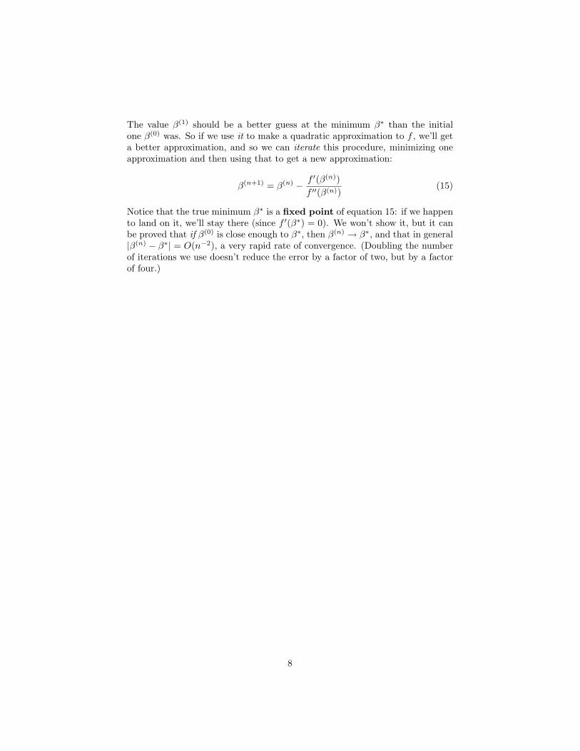
The value β(1) should be a better guess at the minimum β∗ than the initialone β(0) was. So if we use it to make a quadratic approximation to f , we’ll geta better approximation, and so we can iterate this procedure, minimizing oneapproximation and then using that to get a new approximation:
β(n+1) = β(n) − f ′(β(n))f ′′(β(n))
(15)
Notice that the true minimum β∗ is a fixed point of equation 15: if we happento land on it, we’ll stay there (since f ′(β∗) = 0). We won’t show it, but it canbe proved that if β(0) is close enough to β∗, then β(n) → β∗, and that in general|β(n) − β∗| = O(n−2), a very rapid rate of convergence. (Doubling the numberof iterations we use doesn’t reduce the error by a factor of two, but by a factorof four.)
8

Let’s put this together in an algorithm.
my.newton = function(f,f.prime,f.prime2,beta0,tolerance=1e-3,max.iter=50) {beta = beta0old.f = f(beta)iterations = 0made.changes = TRUEwhile(made.changes & (iterations < max.iter)) {iterations <- iterations +1made.changes <- FALSEnew.beta = beta - f.prime(beta)/f.prime2(beta)new.f = f(new.beta)relative.change = abs(new.f - old.f)/old.f -1made.changes = (relative.changes > tolerance)beta = new.betaold.f = new.f}if (made.changes) {warning("Newton’s method terminated before convergence")
}return(list(minimum=beta,value=f(beta),deriv=f.prime(beta),
deriv2=f.prime2(beta),iterations=iterations,converged=!made.changes))
}
The first three arguments here have to all be functions. The fourth argumentis our initial guess for the minimum, β(0). The last arguments keep Newton’smethod from cycling forever: tolerance tells it to stop when the function stopschanging very much (the relative difference between f(β(n)) and f(β(n+1)) issmall), and max.iter tells it to never do more than a certain number of stepsno matter what. The return value includes the estmated minimum, the value ofthe function there, and some diagnostics — the derivative should be very small,the second derivative should be positive, etc.
You may have noticed some potential problems — what if we land on apoint where f ′′ is zero? What if f(β(n+1)) > f(β(n))? Etc. There are ways ofhandling these issues, and more, which are incorporated into real optimizationalgorithms from numerical analysis — such as the optim function in R; I stronglyrecommend you use that, or something like that, rather than trying to roll yourown optimization code.2
3.1 Newton’s Method in More than One Dimension
Suppose that the objective f is a function of multiple arguments, f(β1, β2, . . . βp).Let’s bundle the parameters into a single vector, w. Then the Newton update
2optim actually is a wrapper for several different optimization methods; method=BFGS selectsa Newtonian method; BFGS is an acronym for the names of the algorithm’s inventors.
9
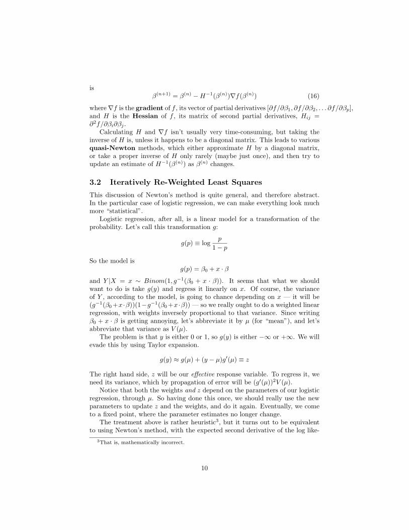
isβ(n+1) = β(n) −H−1(β(n))∇f(β(n)) (16)
where∇f is the gradient of f , its vector of partial derivatives [∂f/∂β1, ∂f/∂β2, . . . ∂f/∂βp],and H is the Hessian of f , its matrix of second partial derivatives, Hij =∂2f/∂βi∂βj .
Calculating H and ∇f isn’t usually very time-consuming, but taking theinverse of H is, unless it happens to be a diagonal matrix. This leads to variousquasi-Newton methods, which either approximate H by a diagonal matrix,or take a proper inverse of H only rarely (maybe just once), and then try toupdate an estimate of H−1(β(n)) as β(n) changes.
3.2 Iteratively Re-Weighted Least Squares
This discussion of Newton’s method is quite general, and therefore abstract.In the particular case of logistic regression, we can make everything look muchmore “statistical”.
Logistic regression, after all, is a linear model for a transformation of theprobability. Let’s call this transformation g:
g(p) ≡ logp
1− p
So the model isg(p) = β0 + x · β
and Y |X = x ∼ Binom(1, g−1(β0 + x · β)). It seems that what we shouldwant to do is take g(y) and regress it linearly on x. Of course, the varianceof Y , according to the model, is going to chance depending on x — it will be(g−1(β0 +x ·β))(1−g−1(β0 +x ·β)) — so we really ought to do a weighted linearregression, with weights inversely proportional to that variance. Since writingβ0 + x · β is getting annoying, let’s abbreviate it by µ (for “mean”), and let’sabbreviate that variance as V (µ).
The problem is that y is either 0 or 1, so g(y) is either −∞ or +∞. We willevade this by using Taylor expansion.
g(y) ≈ g(µ) + (y − µ)g′(µ) ≡ z
The right hand side, z will be our effective response variable. To regress it, weneed its variance, which by propagation of error will be (g′(µ))2V (µ).
Notice that both the weights and z depend on the parameters of our logisticregression, through µ. So having done this once, we should really use the newparameters to update z and the weights, and do it again. Eventually, we cometo a fixed point, where the parameter estimates no longer change.
The treatment above is rather heuristic3, but it turns out to be equivalentto using Newton’s method, with the expected second derivative of the log like-
3That is, mathematically incorrect.
10

lihood, instead of its actual value.4 Since, with a large number of observations,the observed second derivative should be close to the expected second derivative,this is only a small approximation.
4 Generalized Linear Models and GeneralizedAdditive Models
Logistic regression is part of a broader family of generalized linear mod-els (GLMs), where the conditional distribution of the response falls in someparametric family, and the parameters are set by the linear predictor. Ordi-nary, least-squares regression is the case where response is Gaussian, with meanequal to the linear predictor, and constant variance. Logistic regression is thecase where the response is binomial, with n equal to the number of data-pointswith the given x (often but not always 1), and p is given by Equation 2. Chang-ing the relationship between the parameters and the linear predictor is calledchanging the link function. For computational reasons, the link function isactually the function you apply to the mean response to get back the linear pre-dictor, rather than the other way around — (1) rather than (2). There are thusother forms of binomial regression besides logistic regression.5 There is alsoPoisson regression (appropriate when the data are counts without any upperlimit), gamma regression, etc.; we will say more about these next time.
In R, any standard GLM can be fit using the (base) glm function, whosesyntax is very similar to that of lm. The major wrinkle is that, of course, youneed to specify the family of probability distributions to use, by the familyoption — family=binomial defaults to logistic regression. (See help(glm) forthe gory details on how to do, say, probit regression.) All of these are fit by thesame sort of numerical likelihood maximization.
One caution about using maximum likelihood to fit logistic regression is thatit can seem to work badly when the training data can be linearly separated. Thereason is that, to make the likelihood large, p(xi) should be large when yi = 1,and p should be small when yi = 0. If β0, β0 is a set of parameters whichperfectly classifies the training data, then cβ0, cβ is too, for any c > 1, butin a logistic regression the second set of parameters will have more extremeprobabilities, and so a higher likelihood. For linearly separable data, then,there is no parameter vector which maximizes the likelihood, since ` can alwaysbe increased by making the vector larger but keeping it pointed in the samedirection.
4This takes a reasonable amount of algebra to show, so we’ll skip it. The key pointhowever is the following. Take a single Bernoulli observation with success probability p.The log-likelihood is Y log p + (1 − Y ) log 1 − p. The first derivative with respect to p isY/p − (1 − Y )/(1 − p), and the second derivative is −Y/p2 − (1 − Y )/(1 − p)2. Takingexpectations gives −1/p− 1/(1− p) = −1/p(1− p). In other words, V (p) = −1/E [`′′]. Usingweights inversely proportional to the variance thus turns out to be equivalent to dividing bythe expected second derivative.
5My experience is that these tend to give similar error rates as classifiers, but have ratherdifferent guesses about the underlying probabilities.
11
You should, of course, be so lucky as to have this problem.
4.1 Generalized Additive Models
A natural step beyond generalized linear models is generalized additive mod-els (GAMs), where instead of making the transformed mean response a linearfunction of the inputs, we make it an additive function of the inputs. This meanscombining a function for fitting additive models with likelihood maximization.The R function here is gam, from the CRAN package of the same name. (Alter-nately, use the function gam in the package mgcv, which is part of the default Rinstallation.)
GAMs can be used to check GLMs in much the same way that smootherscan be used to check parametric regressions: fit a GAM and a GLM to the samedata, then simulate from the GLM, and re-fit both models to the simulated data.Repeated many times, this gives a distribution for how much better the GAMwill seem to fit than the GLM does, even when the GLM is true. You can thenread a p-value off of this distribution.
4.2 An Example (Including Model Checking)
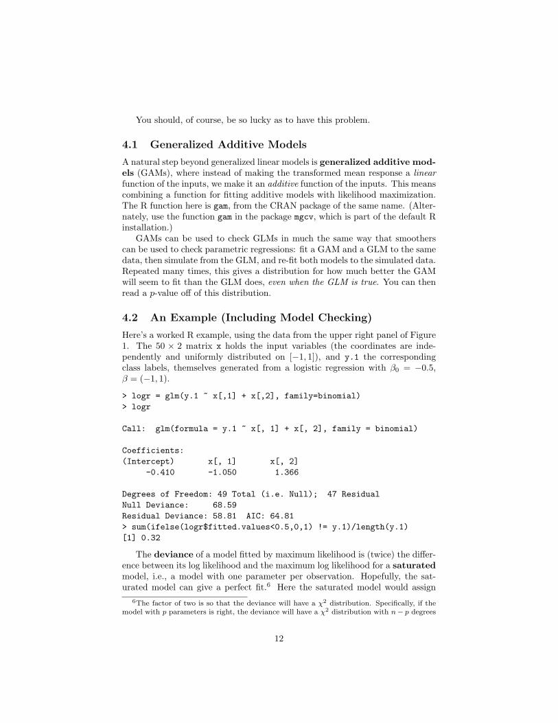
Here’s a worked R example, using the data from the upper right panel of Figure1. The 50 × 2 matrix x holds the input variables (the coordinates are inde-pendently and uniformly distributed on [−1, 1]), and y.1 the correspondingclass labels, themselves generated from a logistic regression with β0 = −0.5,β = (−1, 1).
> logr = glm(y.1 ~ x[,1] + x[,2], family=binomial)> logr
Call: glm(formula = y.1 ~ x[, 1] + x[, 2], family = binomial)
Coefficients:(Intercept) x[, 1] x[, 2]
-0.410 -1.050 1.366
Degrees of Freedom: 49 Total (i.e. Null); 47 ResidualNull Deviance: 68.59Residual Deviance: 58.81 AIC: 64.81> sum(ifelse(logr$fitted.values<0.5,0,1) != y.1)/length(y.1)[1] 0.32
The deviance of a model fitted by maximum likelihood is (twice) the differ-ence between its log likelihood and the maximum log likelihood for a saturatedmodel, i.e., a model with one parameter per observation. Hopefully, the sat-urated model can give a perfect fit.6 Here the saturated model would assign
6The factor of two is so that the deviance will have a χ2 distribution. Specifically, if themodel with p parameters is right, the deviance will have a χ2 distribution with n− p degrees
12

probability 1 to the observed outcomes7, and the logarithm of 1 is zero, soD = 2`(β̂0, β̂). The null deviance is what’s achievable by using just a constantbias b and setting w = 0. The fitted model definitely improves on that.8
The fitted values of the logistic regression are the class probabilities; thisshows that the error rate of the logistic regression, if you force it to predictactual classes, is 32%. This sounds bad, but notice from the contour lines inthe figure that lots of the probabilities are near 0.5, meaning that the classesare just genuinely hard to predict.
To see how well the logistic regression assumption holds up, let’s comparethis to a GAM.
> gam.1 = gam(y.1~lo(x[,1])+lo(x[,2]),family="binomial")> gam.1Call:gam(formula = y.1 ~ lo(x[, 1]) + lo(x[, 2]), family = "binomial")
Degrees of Freedom: 49 total; 41.39957 ResidualResidual Deviance: 49.17522
This fits a GAM to the same data, using lowess smoothing of both input vari-ables. Notice that the residual deviance is lower. That is, the GAM fits better.We expect this; the question is whether the difference is significant, or withinthe range of what we should expect when logistic regression is valid. To testthis, we need to simulate from the logistic regression model.
simulate.from.logr = function(x, coefs) {require(faraway) # For accessible logit and inverse-logit functionsn = nrow(x)linear.part = coefs[1] + x %*% coefs[-1]probs = ilogit(linear.part) # Inverse logity = rbinom(n,size=1,prob=probs)return(y)
}
Now we simulate from our fitted model, and re-fit both the logistic regressionand the GAM.
delta.deviance.sim = function (x,logistic.model) {y.new = simulate.from.logr(x,logistic.model$coefficients)GLM.dev = glm(y.new ~ x[,1] + x[,2], family="binomial")$deviance
of freedom.7This is not possible when there are multiple observations with the same input features,
but different classes.8AIC is of course the Akaike information criterion, −2` + 2q, with q being the number
of parameters (here, q = 3). AIC has some truly devoted adherents, especially among non-statisticians, but I have been deliberately ignoring it and will continue to do so. Claeskensand Hjort (2008) is a thorough, modern treatment of AIC and related model-selection criteriafrom a statistical viewpoint.
13

GAM.dev = gam(y.new ~ lo(x[,1]) + lo(x[,2]), family="binomial")$deviancereturn(GLM.dev - GAM.dev)
}
Notice that in this simulation we are not generating new ~X values. The logisticregression and the GAM are both models for the response conditional on theinputs, and are agnostic about how the inputs are distributed, or even whetherit’s meaningful to talk about their distribution.
Finally, we repeat the simulation a bunch of times, and see where the ob-served difference in deviances falls in the sampling distribution.
> delta.dev = replicate(1000,delta.deviance.sim(x,logr))> delta.dev.observed = logr$deviance - gam.1$deviance # 9.64> sum(delta.dev.observed > delta.dev)/1000[1] 0.685
In other words, the amount by which a GAM fits the data better than logisticregression is pretty near the middle of the null distribution. Since the exampledata really did come from a logistic regression, this is a relief.
References
Claeskens, Gerda and Nils Lid Hjort (2008). Model Selection and Model Aver-aging . Cambridge, England: Cambridge University Press.
14

0 10 20 30
0.00
0.02
0.04
0.06
0.08
0.10
Amount by which GAM fits better than logistic regression
Sampling distribution under logistic regressionN = 1000 Bandwidth = 0.8386
Density
Figure 2: Sampling distribution for the difference in deviance between a GAMand a logistic regression, on data generated from a logistic regression. Theobserved difference in deviances is shown by the dashed horizontal line.
15