149-2010: PROC COMPARE: Worth Another Look!support.sas.com/resources/papers/proceedings10/149-2010.pdf · PROC COMPARE – Worth Another Look! Christianna S. Williams, Abt Associates

Paper 149-2010

PROC COMPARE – Worth Another Look! Christianna S. Williams, Abt Associates Inc, Durham, NC

ABSTRACT

PROC COMPARE is one of those workhorse procedures in the Base SAS® closet that deserves to be dusted off, tuned up and pressed into service again! With well-chosen PROC COMPARE options and statements, you can compare pairs of SAS datasets at multiple levels without the need for DATA step MERGEs or SQL JOINs. Specifically, you can identify differences and similarities across SAS data sets with respect to: data set attributes; variable existence and attributes; existence of matching observations; and variable values (at user-specified levels of precision). This handy PROC can even be used to compare values of one variable to another within a dataset. Additionally, several different reporting options are available and can be customized to project needs. This flexibility makes PROC COMPARE an extremely useful tool for a variety of purposes, including data cleaning and validation, ensuring that new data is consistent with “legacy” data (or differs in expected ways), and even for some simple longitudinal analysis! This tutorial-style paper will teach you how to harness some of the power of this under-appreciated procedure!

INTRODUCTION

I’m not sure if PROC COMPARE existed in the very first version of SAS, but it has certainly been around at least since version 5 – many moons ago. In my opinion, it is one of those ‘oldies but goodies’ that well-rounded SAS programmers need to know about. It is invaluable for the many situations in which one needs to compare two data sets. For example, consider PROC COMPARE the next time you need…

• to evaluate newly collected data in comparison to an existing file;

• to test whether data set updates or edits have occurred as expected;

• to examine whether two algorithms for computing certain variables produce comparable results;

• to prepare for a merge/joint of two large data sets with many variables, so that one knows what variables may need to be renamed.

Of course, much of the functionality of PROC COMPARE could be achieved in other ways, such as joining or merging two data sets, followed by identifying mis-matches and analyzing similarities and differences among variables on matching observations. Indeed, because we are talking about “data set stuff”, rather than statistical analyses, there is the tendency to head first to the DATA step for a solution, rather than considering the sometimes daunting stable of PROCs. However, why not make use of the SAS machinery that is specifically designed for the purpose of comparing of data sets – or at least be familiar enough with its capabilities so that you can consider whether it suits your needs. The purpose of this paper, then, is to introduce (or re-introduce) many of the features of PROC COMPARE through a series of examples, in the hopes that you can add this to your toolkit or deepen your understanding of what can be accomplished with just a few statements.

THE DATA

The data for all the examples in this paper comes from a project I and others at Abt have been working on with the Centers for Medicare and Medicaid (CMS) to generate quality ratings for all US Nursing Homes1. This includes nearly 16,000 nursing homes, and the ratings are updated every month. To simplify things for the purposes of the examples, I’ve limited the data to just nursing homes in Washington state, and, of course, just a small subset of the variables that are used in generating the ratings. To make the comparisons shown in the examples in this paper at least a little bit relevant to real life, I’m using one data set that has information about all certified Washington nursing homes from July 2009 (named WA_jul2009) and another with information about the nursing homes in Washington that were certified in February 2010 (named WA_feb2010). For reference, PROC CONTENTS output for each of these data sets is included in an appendix.

1 Nursing Home Compare: http://www.medicare.gov/NHCompare/

1

Foundations and FundamentalsSAS Global Forum 2010

http://www.medicare.gov/NHCompare/

EXAMPLE 1 – PLAIN VANILLA PROC COMPARE

When getting familiar with a new PROC, I always like to try running it without any options or non-required statements – the bare bones, and then work from there. You probably rarely will want to run the PROC just like this, but it gives you a starting point. So, in this first example, all I am specifying are the two data sets I am comparing, one is the BASE data set and one is the COMPARE data set.

PROC COMPARE BASE=in.WA_jul2009 COMPARE=in.WA_feb2010 ; TITLE1 'Example 1: PROC COMPARE with no options or extra statements'; RUN;

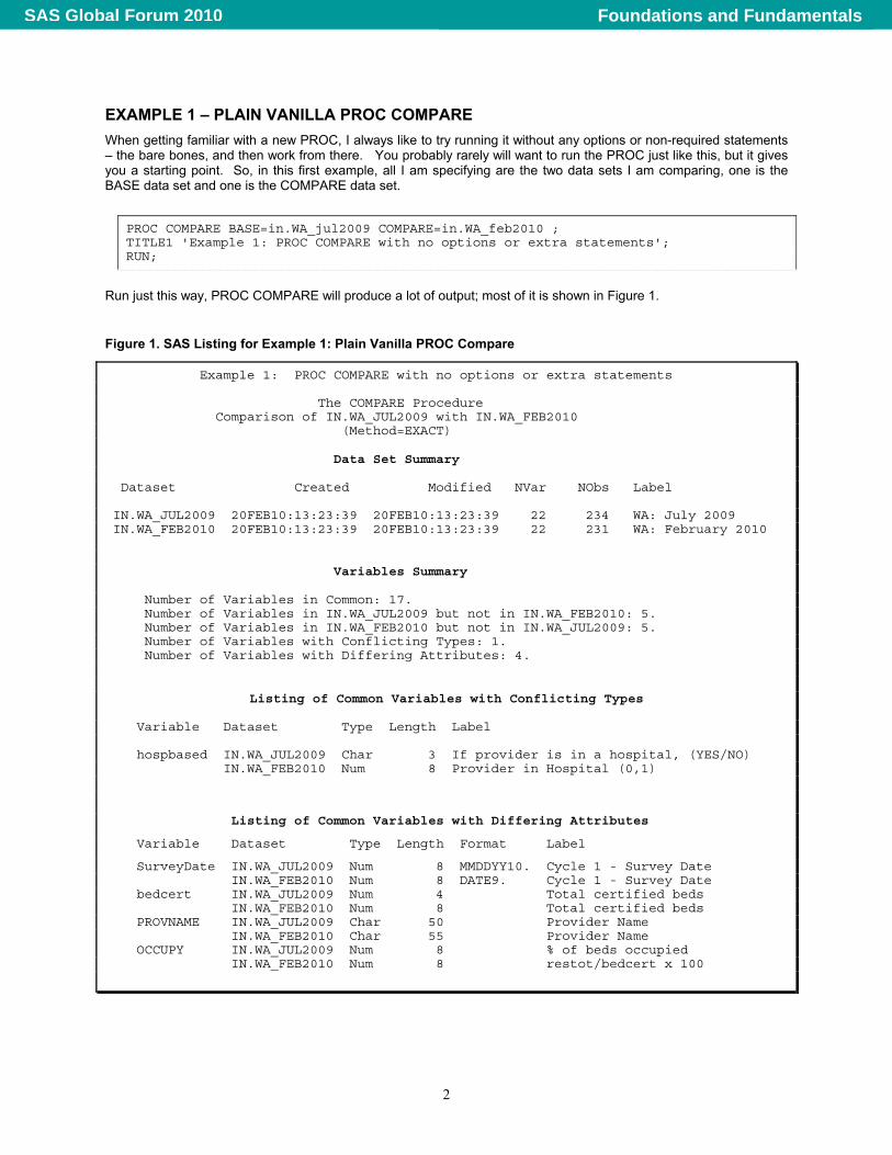
Run just this way, PROC COMPARE will produce a lot of output; most of it is shown in Figure 1.

Figure 1. SAS Listing for Example 1: Plain Vanilla PROC Compare

Example 1: PROC COMPARE with no options or extra statements The COMPARE Procedure Comparison of IN.WA_JUL2009 with IN.WA_FEB2010 (Method=EXACT) Data Set Summary Dataset Created Modified NVar NObs Label IN.WA_JUL2009 20FEB10:13:23:39 20FEB10:13:23:39 22 234 WA: July 2009 IN.WA_FEB2010 20FEB10:13:23:39 20FEB10:13:23:39 22 231 WA: February 2010 Variables Summary Number of Variables in Common: 17. Number of Variables in IN.WA_JUL2009 but not in IN.WA_FEB2010: 5. Number of Variables in IN.WA_FEB2010 but not in IN.WA_JUL2009: 5. Number of Variables with Conflicting Types: 1. Number of Variables with Differing Attributes: 4.

Listing of Common Variables with Conflicting Types

Variable Dataset Type Length Label hospbased IN.WA_JUL2009 Char 3 If provider is in a hospital, (YES/NO) IN.WA_FEB2010 Num 8 Provider in Hospital (0,1)

Listing of Common Variables with Differing Attributes

Variable Dataset Type Length Format Label

SurveyDate IN.WA_JUL2009 Num 8 MMDDYY10. Cycle 1 - Survey Date IN.WA_FEB2010 Num 8 DATE9. Cycle 1 - Survey Date bedcert IN.WA_JUL2009 Num 4 Total certified beds IN.WA_FEB2010 Num 8 Total certified beds PROVNAME IN.WA_JUL2009 Char 50 Provider Name IN.WA_FEB2010 Char 55 Provider Name OCCUPY IN.WA_JUL2009 Num 8 % of beds occupied IN.WA_FEB2010 Num 8 restot/bedcert x 100

2


Observation Summary Observation Base Compare First Obs 1 1 First Unequal 1 1 Last Unequal 231 231 Last Match 231 231 Last Obs 234 . Number of Observations in Common: 231. Number of Observations in IN.WA_JUL2009 but not in IN.WA_FEB2010: 3. Total Number of Observations Read from IN.WA_JUL2009: 234. Total Number of Observations Read from IN.WA_FEB2010: 231. Number of Observations with Some Compared Variables Unequal: 229. Number of Observations with All Compared Variables Equal: 2. Values Comparison Summary Number of Variables Compared with All Observations Equal: 2. Number of Variables Compared with Some Observations Unequal: 14. Number of Variables with Missing Value Differences: 3. Total Number of Values which Compare Unequal: 1942. Maximum Difference: 529. Variables with Unequal Values Variable Type Len1 Len2 Ndif MaxDif MissDif PROVNUM CHAR 10 10 120 0 SurveyDate NUM 8 8 187 529 0 numcycles NUM 8 8 2 1.000 0 defscore NUM 8 8 224 447 0 def5star NUM 8 8 125 4.000 0 MDS5star NUM 4 4 154 4.000 1 rnstf5 NUM 8 8 129 4.000 7 staff5star NUM 8 8 126 4.000 7 PROVNAME CHAR 50 55 123 0 CITY CHAR 28 28 116 0 BEDCERT NUM 8 8 127 158 0 RESTOT NUM 8 8 183 168 0 OCCUPY NUM 8 8 185 42.000 0 Comp5star NUM 8 8 141 4.000 0 Value Comparison Results for Variables __________________________________________________________ || Federal Provider Number || Base Value Compare Value Obs || PROVNUM PROVNUM ________ || __________ __________ || 112 || 505333 505334 113 || 505334 505338 114 || 505338 505339 < snip > 159 || 505409 505411 160 || 505410 505412 161 || 505411 505413 NOTE: The MAXPRINT=50 printing limit has been reached for the variable PROVNUM. No more values will be printed for this comparison. __________________________________________________________

3


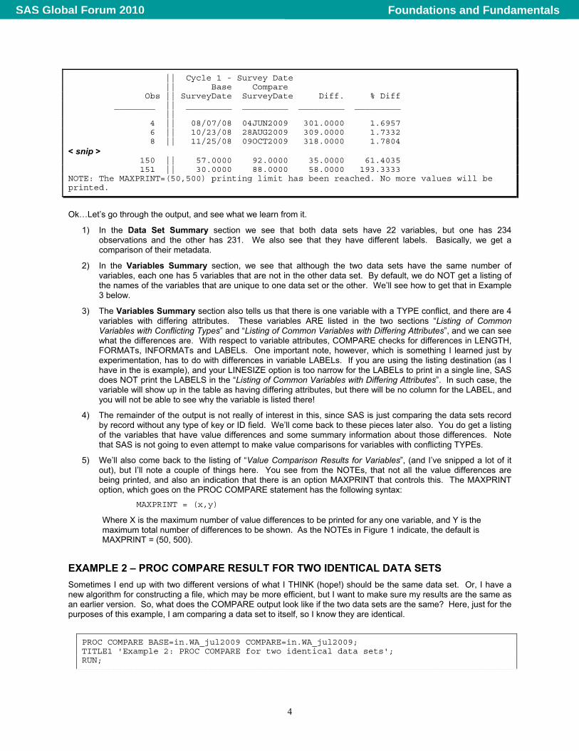
|| Cycle 1 - Survey Date || Base Compare Obs || SurveyDate SurveyDate Diff. % Diff ________ || _________ _________ _________ _________ || 4 || 08/07/08 04JUN2009 301.0000 1.6957 6 || 10/23/08 28AUG2009 309.0000 1.7332 8 || 11/25/08 09OCT2009 318.0000 1.7804 < snip > 150 || 57.0000 92.0000 35.0000 61.4035 151 || 30.0000 88.0000 58.0000 193.3333 NOTE: The MAXPRINT=(50,500) printing limit has been reached. No more values will be printed.

Ok…Let’s go through the output, and see what we learn from it.

1) In the Data Set Summary section we see that both data sets have 22 variables, but one has 234 observations and the other has 231. We also see that they have different labels. Basically, we get a comparison of their metadata.

2) In the Variables Summary section, we see that although the two data sets have the same number of variables, each one has 5 variables that are not in the other data set. By default, we do NOT get a listing of the names of the variables that are unique to one data set or the other. We’ll see how to get that in Example 3 below.

3) The Variables Summary section also tells us that there is one variable with a TYPE conflict, and there are 4 variables with differing attributes. These variables ARE listed in the two sections “Listing of Common Variables with Conflicting Types” and “Listing of Common Variables with Differing Attributes”, and we can see what the differences are. With respect to variable attributes, COMPARE checks for differences in LENGTH, FORMATs, INFORMATs and LABELs. One important note, however, which is something I learned just by experimentation, has to do with differences in variable LABELs. If you are using the listing destination (as I have in the is example), and your LINESIZE option is too narrow for the LABELs to print in a single line, SAS does NOT print the LABELS in the “Listing of Common Variables with Differing Attributes”. In such case, the variable will show up in the table as having differing attributes, but there will be no column for the LABEL, and you will not be able to see why the variable is listed there!

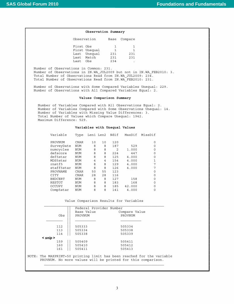
4) The remainder of the output is not really of interest in this, since SAS is just comparing the data sets record by record without any type of key or ID field. We’ll come back to these pieces later also. You do get a listing of the variables that have value differences and some summary information about those differences. Note that SAS is not going to even attempt to make value comparisons for variables with conflicting TYPEs.

5) We’ll also come back to the listing of “Value Comparison Results for Variables”, (and I’ve snipped a lot of it out), but I’ll note a couple of things here. You see from the NOTEs, that not all the value differences are being printed, and also an indication that there is an option MAXPRINT that controls this. The MAXPRINT option, which goes on the PROC COMPARE statement has the following syntax:

MAXPRINT = (x,y)

Where X is the maximum number of value differences to be printed for any one variable, and Y is the maximum total number of differences to be shown. As the NOTEs in Figure 1 indicate, the default is MAXPRINT = (50, 500).

EXAMPLE 2 – PROC COMPARE RESULT FOR TWO IDENTICAL DATA SETS

Sometimes I end up with two different versions of what I THINK (hope!) should be the same data set. Or, I have a new algorithm for constructing a file, which may be more efficient, but I want to make sure my results are the same as an earlier version. So, what does the COMPARE output look like if the two data sets are the same? Here, just for the purposes of this example, I am comparing a data set to itself, so I know they are identical.

PROC COMPARE BASE=in.WA_jul2009 COMPARE=in.WA_jul2009; TITLE1 'Example 2: PROC COMPARE for two identical data sets'; RUN;

4


The output is short and sweet.

Figure 2. SAS Listing for Example 2: Comparison of two identical data sets

Example 2: PROC COMPARE for two identical data sets The COMPARE Procedure Comparison of IN.WA_JUL2009 with IN.WA_JUL2009 (Method=EXACT) Data Set Summary Dataset Created Modified NVar NObs IN.WA_JUL2009 06FEB10:17:32:51 06FEB10:17:32:51 22 234 IN.WA_JUL2009 06FEB10:17:32:51 06FEB10:17:32:51 22 234 Variables Summary Number of Variables in Common: 22. Observation Summary Observation Base Compare First Obs 1 1 Last Obs 234 234 Number of Observations in Common: 234. Total Number of Observations Read from IN.WA_JUL2009: 234. Total Number of Observations Read from IN.WA_JUL2009: 234. Number of Observations with Some Compared Variables Unequal: 0. Number of Observations with All Compared Variables Equal: 234. NOTE: No unequal values were found. All values compared are exactly equal.

EXAMPLE 3 – WHEN ALL YOU REALLY CARE ABOUT IS THE CONTENTS: PROC COMPARE WITH NOVALUES, LISTVAR AND BRIEF OPTIONS

We often get data sets from a client that have updated data, but are otherwise supposed to be the same (that is, they have the same variables, and those variables have the same attributes and meaning). Now, of course, you could do a PROC CONTENTS of each data set, and match them up and see if they are the same – and this may very well be worth doing, but PROC COMPARE also allows for a “quick and dirty” comparison of this metadata. So, when you do not want to compare the values of variables, you can use the NOVALUES option on the PROC COMPARE statement. I’m also including the LISTVAR option, which I’ll explain below. Otherwise, this code is identical to that shown in Example 1.

PROC COMPARE BASE=in.WA_jul2009 COMPARE=in.WA_feb2010 NOVALUES LISTVAR; TITLE1 'Example : PROC COMPARE with NOVALUES & LISTVAR options'; RUN;

If I did not include the LISTVAR option, the output that will be produced will be identical to that shown in Figure 1, except it will stop after the table titled “Variables with Unequal Values”. So, you will still get a listing of the variables that have unequal values, but you won’t get listings of the specific value differences. And, without LISTVAR you would also not get a listing of the names of the variables that are unique to one data set or the other – and likely this information is of interest. Figure 3 shows the additional information that LISTVAR produces; this section of output will come after the Variables Summary and before the Listing of Variables with Conflicting Types.

5


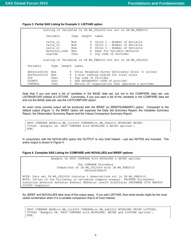
Figure 3. Partial SAS Listing for Example 3: LISTVAR option

Listing of Variables in IN.WA_JUL2009 but not in IN.WA_FEB2010 Variable Type Length Label revis_c1 Num 8 Cycle 1 - Number of Revisits revis_c2 Num 8 Cycle 2 - Number of Revisits revis_c3 Num 8 Cycle 3 - Number of Revisits defscore_rank Num 8 Rank for Variable defscore zipcode Char 5 Zip code of Provider

Listing of Variables in IN.WA_FEB2010 but not in IN.WA_JUL2009 Variable Type Length Label defscore0104 Num 8 Total Weighted Survey Deficiency Score (3 cycles) def5star0104 Num 8 5-star ranking system for total score ZIP Char 5 Zip code of Provider COUNTY Char 3 SSA GEOGRAPHIC CODE of provider CONTROL Char 2 Nature of organization that operates a provider

Note that if you just want a list of variables in the BASE data set, but not in the COMPARE data set, use LISTBASEVAR instead of LISTVAR. Conversely, if you just want a list of the variables in the COMPARE data set and not the BASE data set, use the LISTCOMPVAR option.

An even more concise output will be produced with the BRIEF (or BRIEFSUMMARY) option. Compared to the default output (Figure 1), the BRIEF option will suppress the Data Set Summary Report, the Variables Summary Report, the Observation Summary Report and the Values Comparison Summary Report.

PROC COMPARE BASE=in.WA_jul2009 COMPARE=in.WA_feb2010 NOVALUES BRIEF; TITLE1 'Example 3A: PROC COMPARE with NOVALUES & BRIEF options'; RUN;

In conjunction with the NOVALUES option the OUTPUT is very brief indeed – just two NOTES are included. The entire output is shown in Figure 4.

Figure 4. Complete SAS Listing for COMPARE with NOVALUES and BRIEF options

Example 3A PROC COMPARE with NOVALUES & BRIEF options

The COMPARE Procedure Comparison of IN.WA_JUL2009 with IN.WA_FEB2010

(Method=EXACT) NOTE: Data set IN.WA_JUL2009 contains 3 observations not in IN.WA_FEB2010. NOTE: Values of the following 14 variables compare unequal: PROVNUM SurveyDate numcycles defscore def5star bedcert MDS5star rnstf5 staff5star PROVNAME CITY RESTOT OCCUPY Comp5star

So, BRIEF and NOVALUES take most of the output away. If you add LISTVAR, then what results might be the most useful combination when it is a variable comparison that is of most interest.

PROC COMPARE BASE=in.WA_jul2009 COMPARE=in.WA_feb2010 NOVALUES BRIEF LISTVAR; TITLE1 'Example 3B: PROC COMPARE with NOVALUES, BRIEF and LISTVAR options'; RUN;

6


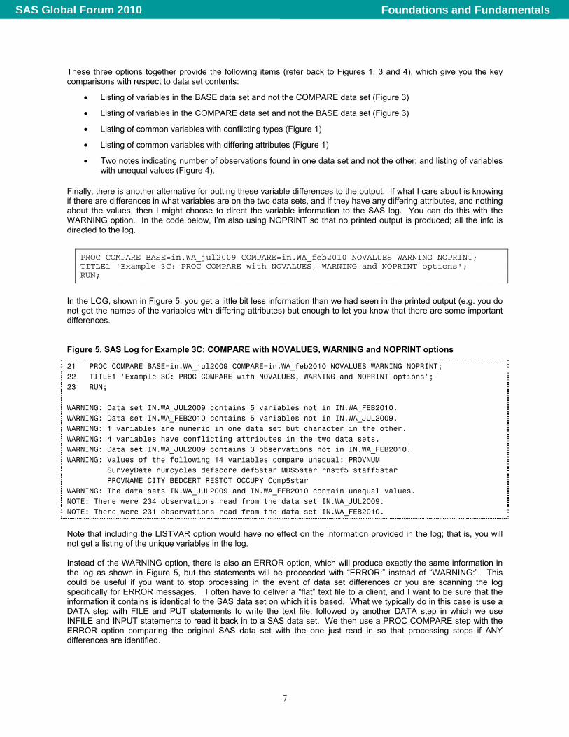
These three options together provide the following items (refer back to Figures 1, 3 and 4), which give you the key comparisons with respect to data set contents:

• Listing of variables in the BASE data set and not the COMPARE data set (Figure 3)

• Listing of variables in the COMPARE data set and not the BASE data set (Figure 3)

• Listing of common variables with conflicting types (Figure 1)

• Listing of common variables with differing attributes (Figure 1)

• Two notes indicating number of observations found in one data set and not the other; and listing of variables with unequal values (Figure 4).

Finally, there is another alternative for putting these variable differences to the output. If what I care about is knowing if there are differences in what variables are on the two data sets, and if they have any differing attributes, and nothing about the values, then I might choose to direct the variable information to the SAS log. You can do this with the WARNING option. In the code below, I’m also using NOPRINT so that no printed output is produced; all the info is directed to the log.

PROC COMPARE BASE=in.WA_jul2009 COMPARE=in.WA_feb2010 NOVALUES WARNING NOPRINT; TITLE1 'Example 3C: PROC COMPARE with NOVALUES, WARNING and NOPRINT options'; RUN;

In the LOG, shown in Figure 5, you get a little bit less information than we had seen in the printed output (e.g. you do not get the names of the variables with differing attributes) but enough to let you know that there are some important differences.

Figure 5. SAS Log for Example 3C: COMPARE with NOVALUES, WARNING and NOPRINT options

21 PROC COMPARE BASE=in.WA_jul2009 COMPARE=in.WA_feb2010 NOVALUES WARNING NOPRINT; 22 TITLE1 'Example 3C: PROC COMPARE with NOVALUES, WARNING and NOPRINT options'; 23 RUN; WARNING: Data set IN.WA_JUL2009 contains 5 variables not in IN.WA_FEB2010. WARNING: Data set IN.WA_FEB2010 contains 5 variables not in IN.WA_JUL2009. WARNING: 1 variables are numeric in one data set but character in the other. WARNING: 4 variables have conflicting attributes in the two data sets. WARNING: Data set IN.WA_JUL2009 contains 3 observations not in IN.WA_FEB2010. WARNING: Values of the following 14 variables compare unequal: PROVNUM SurveyDate numcycles defscore def5star MDS5star rnstf5 staff5star PROVNAME CITY BEDCERT RESTOT OCCUPY Comp5star WARNING: The data sets IN.WA_JUL2009 and IN.WA_FEB2010 contain unequal values. NOTE: There were 234 observations read from the data set IN.WA_JUL2009. NOTE: There were 231 observations read from the data set IN.WA_FEB2010. Note that including the LISTVAR option would have no effect on the information provided in the log; that is, you will not get a listing of the unique variables in the log. Instead of the WARNING option, there is also an ERROR option, which will produce exactly the same information in the log as shown in Figure 5, but the statements will be proceeded with “ERROR:” instead of “WARNING:”. This could be useful if you want to stop processing in the event of data set differences or you are scanning the log specifically for ERROR messages. I often have to deliver a “flat” text file to a client, and I want to be sure that the information it contains is identical to the SAS data set on which it is based. What we typically do in this case is use a DATA step with FILE and PUT statements to write the text file, followed by another DATA step in which we use INFILE and INPUT statements to read it back in to a SAS data set. We then use a PROC COMPARE step with the ERROR option comparing the original SAS data set with the one just read in so that processing stops if ANY differences are identified.

7


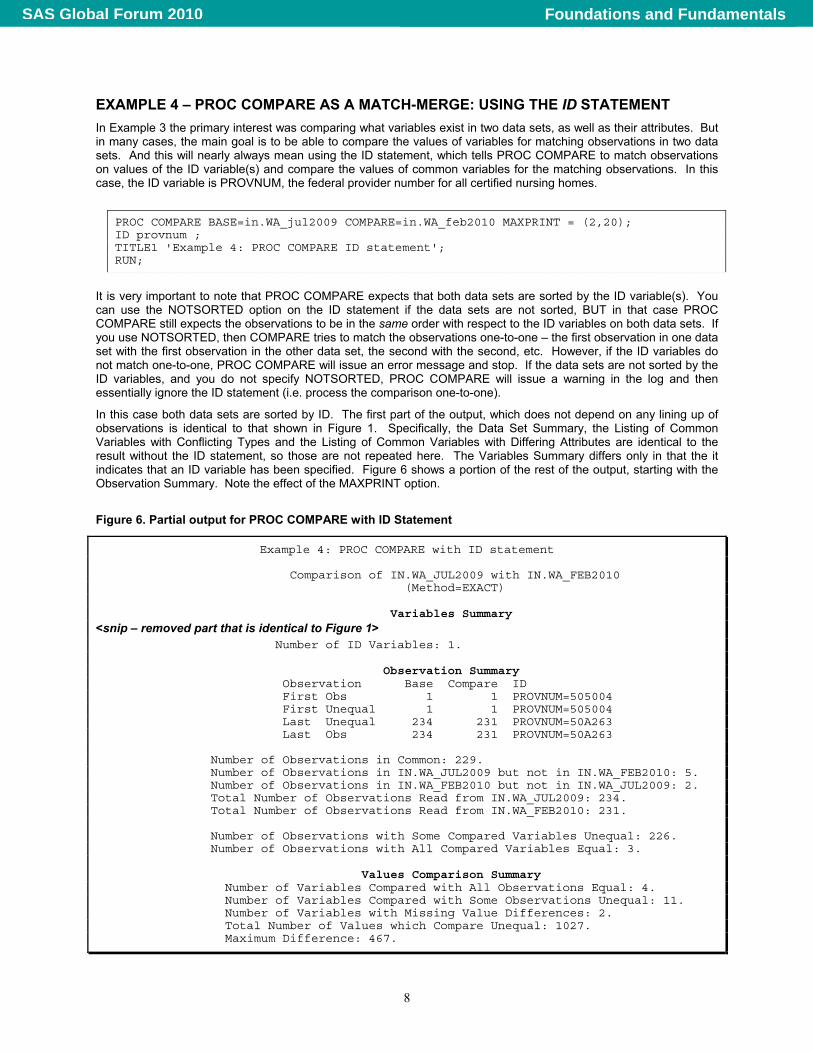
EXAMPLE 4 – PROC COMPARE AS A MATCH-MERGE: USING THE ID STATEMENT

In Example 3 the primary interest was comparing what variables exist in two data sets, as well as their attributes. But in many cases, the main goal is to be able to compare the values of variables for matching observations in two data sets. And this will nearly always mean using the ID statement, which tells PROC COMPARE to match observations on values of the ID variable(s) and compare the values of common variables for the matching observations. In this case, the ID variable is PROVNUM, the federal provider number for all certified nursing homes.

PROC COMPARE BASE=in.WA_jul2009 COMPARE=in.WA_feb2010 MAXPRINT = (2,20); ID provnum ; TITLE1 'Example 4: PROC COMPARE ID statement'; RUN;

It is very important to note that PROC COMPARE expects that both data sets are sorted by the ID variable(s). You can use the NOTSORTED option on the ID statement if the data sets are not sorted, BUT in that case PROC COMPARE still expects the observations to be in the same order with respect to the ID variables on both data sets. If you use NOTSORTED, then COMPARE tries to match the observations one-to-one – the first observation in one data set with the first observation in the other data set, the second with the second, etc. However, if the ID variables do not match one-to-one, PROC COMPARE will issue an error message and stop. If the data sets are not sorted by the ID variables, and you do not specify NOTSORTED, PROC COMPARE will issue a warning in the log and then essentially ignore the ID statement (i.e. process the comparison one-to-one).

In this case both data sets are sorted by ID. The first part of the output, which does not depend on any lining up of observations is identical to that shown in Figure 1. Specifically, the Data Set Summary, the Listing of Common Variables with Conflicting Types and the Listing of Common Variables with Differing Attributes are identical to the result without the ID statement, so those are not repeated here. The Variables Summary differs only in that the it indicates that an ID variable has been specified. Figure 6 shows a portion of the rest of the output, starting with the Observation Summary. Note the effect of the MAXPRINT option.

Figure 6. Partial output for PROC COMPARE with ID Statement

Example 4: PROC COMPARE with ID statement Comparison of IN.WA_JUL2009 with IN.WA_FEB2010 (Method=EXACT) Variables Summary <snip – removed part that is identical to Figure 1> Number of ID Variables: 1. Observation Summary Observation Base Compare ID First Obs 1 1 PROVNUM=505004 First Unequal 1 1 PROVNUM=505004 Last Unequal 234 231 PROVNUM=50A263 Last Obs 234 231 PROVNUM=50A263 Number of Observations in Common: 229. Number of Observations in IN.WA_JUL2009 but not in IN.WA_FEB2010: 5. Number of Observations in IN.WA_FEB2010 but not in IN.WA_JUL2009: 2. Total Number of Observations Read from IN.WA_JUL2009: 234. Total Number of Observations Read from IN.WA_FEB2010: 231. Number of Observations with Some Compared Variables Unequal: 226. Number of Observations with All Compared Variables Equal: 3. Values Comparison Summary Number of Variables Compared with All Observations Equal: 4. Number of Variables Compared with Some Observations Unequal: 11. Number of Variables with Missing Value Differences: 2. Total Number of Values which Compare Unequal: 1027. Maximum Difference: 467.

8


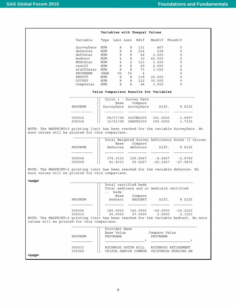
Variables with Unequal Values Variable Type Len1 Len2 Ndif MaxDif MissDif SurveyDate NUM 8 8 131 467 0 defscore NUM 8 8 214 238 0 def5star NUM 8 8 64 2.000 0 bedcert NUM 4 8 15 40.000 0 MDS5star NUM 4 4 123 3.000 0 rnstf5 NUM 8 8 69 2.000 4 staff5star NUM 8 8 73 3.000 4 PROVNAME CHAR 50 55 4 0 RESTOT NUM 8 8 118 24.000 0 OCCUPY NUM 8 8 122 30.000 0 Comp5star NUM 8 8 94 3.000 0 Value Comparison Results for Variables ____________________________________________________________ || Cycle 1 - Survey Date || Base Compare PROVNUM || SurveyDate SurveyDate Diff. % Diff __________ || _________ _________ _________ _________ || 505016 || 08/07/08 04JUN2009 301.0000 1.6957 505024 || 10/23/08 28AUG2009 309.0000 1.7332 NOTE: The MAXPRINT=2 printing limit has been reached for the variable SurveyDate. No more values will be printed for this comparison. ___________________________________________________________ || Total Weighted Survey Deficiency Score (3 cycles) || Base Compare PROVNUM || defscore defscore Diff. % Diff __________ || _________ _________ _________ _________ || 505004 || 174.3333 169.6667 -4.6667 -2.6769 505009 || 81.8333 59.6667 -22.1667 -27.0876 NOTE: The MAXPRINT=2 printing limit has been reached for the variable defscore. No more values will be printed for this comparison. <snip> ___________________________________________________________ || Total certified beds || Total medicare and or medicaid certified || .. beds || Base Compare PROVNUM || bedcert BEDCERT Diff. % Diff __________ || _________ _________ _________ _________ || 505004 || 180.0000 140.0000 -40.0000 -22.2222 505010 || 95.0000 97.0000 2.0000 2.1053 NOTE: The MAXPRINT=2 printing limit has been reached for the variable bedcert. No more values will be printed for this comparison. ____________________________________________________________ || Provider Name || Base Value Compare Value PROVNUM || PROVNAME PROVNAME __________ || ___________________+ ___________________+ || 505033 || ROCKWOOD SOUTH HILL ROCKWOOD RETIREMENT 505069 || CRISTA SENIOR COMMUN CRISTWOOD NURSING AN <snip>

9


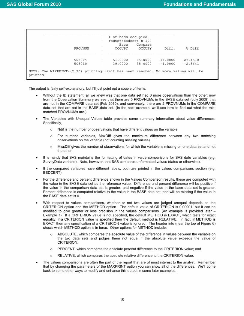
____________________________________________________________ || % of beds occupied || restot/bedcert x 100 || Base Compare PROVNUM || OCCUPY OCCUPY Diff. % Diff __________ || _________ _________ _________ _________ || 505004 || 51.0000 65.0000 14.0000 27.4510 505010 || 39.0000 38.0000 -1.0000 -2.5641 NOTE: The MAXPRINT=(2,20) printing limit has been reached. No more values will be printed.

The output is fairly self-explanatory, but I’ll just point out a couple of items.

• Without the ID statement, all we knew was that one data set had 3 more observations than the other; now from the Observation Summary we see that there are 5 PROVNUMs in the BASE data set (July 2009) that are not in the COMPARE data set (Feb 2010), and conversely, there are 2 PROVNUMs in the COMPARE data set that are not in the BASE data set. (In the next example, we’ll see how to find out what the mis-matched PROVNUMs are.)

• The Variables with Unequal Values table provides some summary information about value differences. Specifically,

o Ndif is the number of observations that have different values on the variable

o For numeric variables, MaxDiff gives the maximum difference between any two matching observations on the variable (not counting missing values).

o MissDiff gives the number of observations for which the variable is missing on one data set and not the other.

• It is handy that SAS maintains the formatting of dates in value comparisons for SAS date variables (e.g. SurveyDate variable). Note, however, that SAS compares unformatted values (dates or otherwise).

• If the compared variables have different labels, both are printed in the values comparisons section (e.g. BEDCERT).

• For the difference and percent difference shown in the Values Comparison results, these are computed with the value in the BASE data set as the reference value. Difference and percent difference will be positive if the value in the comparison data set is greater, and negative if the value in the base data set is greater. Percent difference is computed relative to the value in the BASE data set, and will be missing if the value in the BASE data set is 0.

• With respect to values comparisons, whether or not two values are judged unequal depends on the CRITERION option and the METHOD option. The default value of CRITERION is 0.00001, but it can be modified to give greater or less precision in the values comparisons. (An example is provided later – Example 7). If a CRITERION value is not specified, the default METHOD is EXACT, which tests for exact equality; if a CRITERION value is specified then the default method is RELATIVE. In fact, if METHOD is EXACT then any specification of a CRITERION value is ignored. The header info (near the top of Figure 6) shows which METHOD option is in force. Other options for METHOD include:

o ABSOLUTE, which compares the absolute value of the difference in values between the variable on the two data sets and judges them not equal if the absolute value exceeds the value of CRITERION;

o PERCENT, which compares the absolute percent difference to the CRITERION value; and

o RELATIVE, which compares the absolute relative difference to the CRITERION value.

• The values comparisons are often the part of the report that are of most interest to the analyst. Remember that by changing the parameters of the MAXPRINT option you can show all of the differences. We’ll come back to some other ways to modify and enhance this output in some later examples.

10


EXAMPLE 5 – USING THE ID STATEMENT WITH LISTOBS, AND LISTEQUALVAR

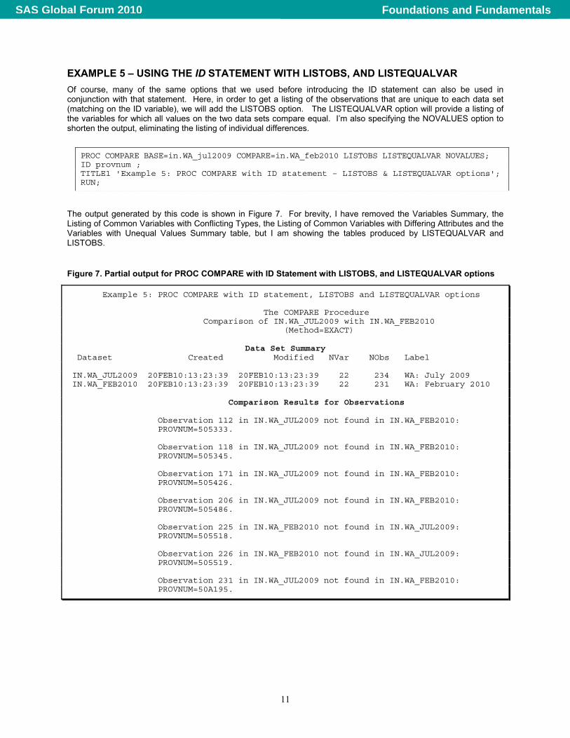
Of course, many of the same options that we used before introducing the ID statement can also be used in conjunction with that statement. Here, in order to get a listing of the observations that are unique to each data set (matching on the ID variable), we will add the LISTOBS option. The LISTEQUALVAR option will provide a listing of the variables for which all values on the two data sets compare equal. I’m also specifying the NOVALUES option to shorten the output, eliminating the listing of individual differences.

PROC COMPARE BASE=in.WA_jul2009 COMPARE=in.WA_feb2010 LISTOBS LISTEQUALVAR NOVALUES; ID provnum ; TITLE1 'Example 5: PROC COMPARE with ID statement – LISTOBS & LISTEQUALVAR options'; RUN;

The output generated by this code is shown in Figure 7. For brevity, I have removed the Variables Summary, the Listing of Common Variables with Conflicting Types, the Listing of Common Variables with Differing Attributes and the Variables with Unequal Values Summary table, but I am showing the tables produced by LISTEQUALVAR and LISTOBS.

Figure 7. Partial output for PROC COMPARE with ID Statement with LISTOBS, and LISTEQUALVAR options

Example 5: PROC COMPARE with ID statement, LISTOBS and LISTEQUALVAR options The COMPARE Procedure Comparison of IN.WA_JUL2009 with IN.WA_FEB2010 (Method=EXACT)

Data Set Summary Dataset Created Modified NVar NObs Label IN.WA_JUL2009 20FEB10:13:23:39 20FEB10:13:23:39 22 234 WA: July 2009 IN.WA_FEB2010 20FEB10:13:23:39 20FEB10:13:23:39 22 231 WA: February 2010 Comparison Results for Observations Observation 112 in IN.WA_JUL2009 not found in IN.WA_FEB2010: PROVNUM=505333. Observation 118 in IN.WA_JUL2009 not found in IN.WA_FEB2010: PROVNUM=505345. Observation 171 in IN.WA_JUL2009 not found in IN.WA_FEB2010: PROVNUM=505426. Observation 206 in IN.WA_JUL2009 not found in IN.WA_FEB2010: PROVNUM=505486. Observation 225 in IN.WA_FEB2010 not found in IN.WA_JUL2009: PROVNUM=505518. Observation 226 in IN.WA_FEB2010 not found in IN.WA_JUL2009: PROVNUM=505519. Observation 231 in IN.WA_JUL2009 not found in IN.WA_FEB2010: PROVNUM=50A195.

11


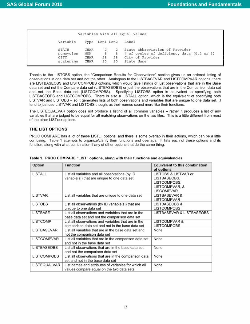
Variables with All Equal Values Variable Type Len1 Len2 Label STATE CHAR 2 2 State abbreviation of Provider numcycles NUM 8 8 # of cycles of deficiency data (0,2 or 3) CITY CHAR 28 28 City of Provider statename CHAR 20 20 State Name

Thanks to the LISTOBS option, the “Comparison Results for Observations” section gives us an ordered listing of observations in one data set and not the other. Analogous to the LISTBASEVAR and LISTCOMPVAR options, there are LISTBASEOBS and LISTCOMPOBS options, which would give listings of just observations that are in the Base data set and not the Compare data set (LISTBASEOBS) or just the observations that are in the Comparison data set and not the Base data set (LISTCOMPOBS). Specifying LISTOBS option is equivalent to specifying both LISTBASEOBS and LISTCOMPOBS. There is also a LISTALL option, which is the equivalent of specifying both LISTVAR and LISTOBS – so it generates lists of both observations and variables that are unique to one data set…I tend to just use LISTVAR and LISTOBS though, as their names sound more like their functions.

The LISTEQUALVAR option does not produce a listing of all common variables – rather it produces a list of any variables that are judged to be equal for all matching observations on the two files. This is a little different from most of the other LISTxxx options.

THE LIST OPTIONS

PROC COMPARE has a lot of these LIST… options, and there is some overlap in their actions, which can be a little confusing. Table 1 attempts to organize/clarify their functions and overlaps. It lists each of these options and its function, along with what combination if any of other options that do the same thing.

Table 1. PROC COMPARE “LIST” options, along with their functions and equivalencies

Option Function Equivalent to this combination of options

LISTALL List all variables and all observations (by ID variable[s]) that are unique to one data set

LISTOBS & LISTVAR or LISTBASEOBS, LISTCOMPOBS, LISTCOMPVAR, & LISCOMPVAR

LISTVAR List all variables that are unique to one data set LISTBASEVAR & LISTCOMPVAR

LISTOBS List all observations (by ID variable[s]) that are unique to one data set

LISTBASEOBS & LISTCOMPOBS

LISTBASE List all observations and variables that are in the base data set and not the comparison data set

LISTBASEVAR & LISTBASEOBS

LISTCOMP List all observations and variables that are in the comparison data set and not in the base data set

LISTCOMPVAR & LISTCOMPOBS

LISTBASEVAR List all variables that are in the base data set and not the comparison data set

None

LISTCOMPVAR List all variables that are in the comparison data set and not in the base data set

None

LISTBASEOBS List all observations that are in the base data set and not the comparison data set

None

LISTCOMPOBS List all observations that are in the comparison data set and not in the base data set

None

LISTEQUALVAR List names and attributes of variables for which all values compare equal on the two data sets

None

12


EXAMPLE 6 – COMPARING VALUES FOR ONLY SELECTED VARIABLES (VAR STATEMENT)

Up to this point, PROC COMPARE has been doing a comparison of values for all matching variables on the two data sets (even if I haven’t been showing ALL the output). However, there will be many cases in which you really just care about differences in a few variables. For this purpose, PROC COMPARE has the VAR statement (and the WITH statement to which we’ll return in a later example. In this example, I am just comparing values for two of the nursing home 5-star ratings – the one for health inspections (DEF5STAR) and the one for staffing (STAFF5STAR). Also, I am including the ALLSTATS option, which will produce some summary information about differences in the variables included in the VAR statement.

PROC COMPARE BASE=in.WA_jul2009 COMPARE=in.WA_feb2010 ALLSTATS MAXPRINT = (3,6); TITLE1 'Example 6: Comparing values only for selected variables'; ID provnum; VAR def5star staff5star; RUN;

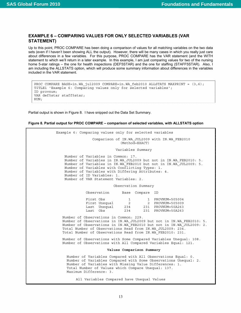
Partial output is shown in Figure 8. I have snipped out the Data Set Summary.

Figure 8. Partial output for PROC COMPARE – comparison of selected variables, with ALLSTATS option

Example 6: Comparing values only for selected variables Comparison of IN.WA_JUL2009 with IN.WA_FEB2010 (Method=EXACT) Variables Summary Number of Variables in Common: 17. Number of Variables in IN.WA_JUL2009 but not in IN.WA_FEB2010: 5. Number of Variables in IN.WA_FEB2010 but not in IN.WA_JUL2009: 5. Number of Variables with Conflicting Types: 1. Number of Variables with Differing Attributes: 4. Number of ID Variables: 1. Number of VAR Statement Variables: 2. Observation Summary Observation Base Compare ID First Obs 1 1 PROVNUM=505004 First Unequal 2 2 PROVNUM=505009 Last Unequal 234 231 PROVNUM=50A263 Last Obs 234 231 PROVNUM=50A263 Number of Observations in Common: 229. Number of Observations in IN.WA_JUL2009 but not in IN.WA_FEB2010: 5. Number of Observations in IN.WA_FEB2010 but not in IN.WA_JUL2009: 2. Total Number of Observations Read from IN.WA_JUL2009: 234. Total Number of Observations Read from IN.WA_FEB2010: 231. Number of Observations with Some Compared Variables Unequal: 108. Number of Observations with All Compared Variables Equal: 121.

Values Comparison Summary Number of Variables Compared with All Observations Equal: 0. Number of Variables Compared with Some Observations Unequal: 2. Number of Variables with Missing Value Differences: 1. Total Number of Values which Compare Unequal: 137. Maximum Difference: 3.

All Variables Compared have Unequal Values

13


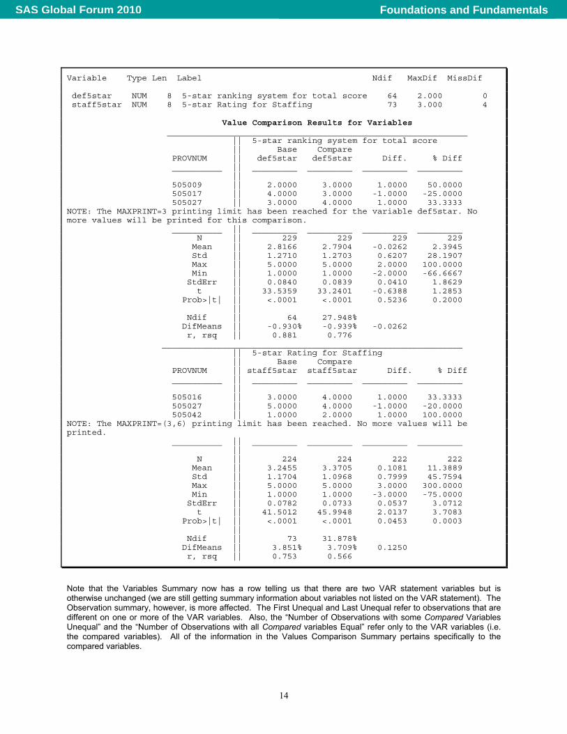
Variable Type Len Label Ndif MaxDif MissDif def5star NUM 8 5-star ranking system for total score 64 2.000 0 staff5star NUM 8 5-star Rating for Staffing 73 3.000 4 Value Comparison Results for Variables ____________________________________________________________ || 5-star ranking system for total score || Base Compare PROVNUM || def5star def5star Diff. % Diff __________ || _________ _________ _________ _________ || 505009 || 2.0000 3.0000 1.0000 50.0000 505017 || 4.0000 3.0000 -1.0000 -25.0000 505027 || 3.0000 4.0000 1.0000 33.3333 NOTE: The MAXPRINT=3 printing limit has been reached for the variable def5star. No more values will be printed for this comparison. __________ || _________ _________ _________ _________ N || 229 229 229 229 Mean || 2.8166 2.7904 -0.0262 2.3945 Std || 1.2710 1.2703 0.6207 28.1907 Max || 5.0000 5.0000 2.0000 100.0000 Min || 1.0000 1.0000 -2.0000 -66.6667 StdErr || 0.0840 0.0839 0.0410 1.8629 t || 33.5359 33.2401 -0.6388 1.2853 Prob>|t| || <.0001 <.0001 0.5236 0.2000 || Ndif || 64 27.948% DifMeans || -0.930% -0.939% -0.0262 r, rsq || 0.881 0.776 ____________________________________________________________ || 5-star Rating for Staffing || Base Compare PROVNUM || staff5star staff5star Diff. % Diff __________ || _________ _________ _________ _________ || 505016 || 3.0000 4.0000 1.0000 33.3333 505027 || 5.0000 4.0000 -1.0000 -20.0000 505042 || 1.0000 2.0000 1.0000 100.0000 NOTE: The MAXPRINT=(3,6) printing limit has been reached. No more values will be printed. __________ || _________ _________ _________ _________ || N || 224 224 222 222 Mean || 3.2455 3.3705 0.1081 11.3889 Std || 1.1704 1.0968 0.7999 45.7594 Max || 5.0000 5.0000 3.0000 300.0000 Min || 1.0000 1.0000 -3.0000 -75.0000 StdErr || 0.0782 0.0733 0.0537 3.0712 t || 41.5012 45.9948 2.0137 3.7083 Prob>|t| || <.0001 <.0001 0.0453 0.0003 || Ndif || 73 31.878% DifMeans || 3.851% 3.709% 0.1250 r, rsq || 0.753 0.566

Note that the Variables Summary now has a row telling us that there are two VAR statement variables but is otherwise unchanged (we are still getting summary information about variables not listed on the VAR statement). The Observation summary, however, is more affected. The First Unequal and Last Unequal refer to observations that are different on one or more of the VAR variables. Also, the “Number of Observations with some Compared Variables Unequal” and the “Number of Observations with all Compared variables Equal” refer only to the VAR variables (i.e. the compared variables). All of the information in the Values Comparison Summary pertains specifically to the compared variables.

14


Let’s look a little more carefully at the summary information produced by the ALLSTATS option. The N row for each variable gives the number of non-missing values; then N value for the “Diff.” And “% Diff” columns gives the number of matching values that can be compared (i.e. non-missing in both data sets) – the fact that (for the variable STAFF5STAR) this number is less than the 224 shown for each data set is an indication that the variable is occasionally missing for one data set and not for the other . The Mean, Std, Max, Min StdErr, t and Prob > |t| rows give, respectively, the mean, standard deviation, maximum, minimum, the standard error of the mean, the t statistic (mean/stderr), and the probability that t would be greater if the population mean was 0. Under the Diff and %Diff columns these statistics refer to the paired differences, which may provide some useful information. For example, for the STAFF5STAR variable, the fact that the mean of the differences is positive (0.1081) indicates that these ratings have, on average, risen between July 2009 and February 2010. Further, the fact that the Prob>|t| value is 0.0453 indicates that this improvement is likely greater than that expected by chance alone – this is a paired t-test. So, we’ve accomplished a little longitudinal analysis!!

What about the 3 rows at the bottom – Ndif, DifMeans and r, rsq? Ndif gives the number (and percent) of values for the variable that are different on the two data sets. The DifMeans row gives the difference between the mean values on the two datasets, first expressed as a percentage of the base mean, second as a percentage of the comparison mean and finally simply the difference in the two means. Analytically, it is important to see why this value (0.1250 for STAFF5STAR) is different from the mean of the differences (0.1081). The DifMeans value (0.1250) just takes the difference in the two sample means, which will differ from the mean of the paired differences (0.1081) because the latter is based on the only those where the value is non-missing in both cases – and this is what one wants when the interest is examining how individual facilities change rather than the overall sample of facilities. Finally, the r and rsq values are the Pearson correlation and its square (i.e. R-square) of the matching non-missing values for the variable between the two data sets – it can be viewed as a crude measure of the autocorrelation over the six month period between the two sets of ratings.

OPTIONS FOR HANDLING MISSING VALUES

The issue of missing values came up several times in explaining these statistics; so it’s worthwhile to explore this area a little further. PROC COMPARE offers several different options for how missing values are treated in the values comparisons. By default, a missing value in one data set will be judged unequal to any non-missing value in the other dataset, and further, missing values will be judged equal only to missing values of the same kind. For example . = ., but . .A and .A = .A, but .A .B, and so on. The three options to change handling of missing values are NOMISSBASE, NOMISSCOMP and NOMISSING:

• NOMISSBASE judges a missing value in the base data set equal to any value in the comparison data set.

• NOMISSCOMP judges a missing value in the comparison data set equal to any value in the base data set.

• NOMISSING judges missing values in either data set equal to any value in the other data set.

The NOMISSBASE and NOMISSCOMP options can be used to evaluate what changes would be made to a master data set in an UPDATE step since missing values on the transaction data set do not overwrite non-missing values on the master dataset. Hence, if you run a PROC COMPARE with the NOMISSCOMP option, you will get a listing only of non-missing values in the comparison data set that differ from the values on the matching observations on the base data set, giving you insight into the expected results of an UPDATE step in which the base data set was the master and the comparison data set was the transaction file.

Here we just tweak the previous example a little by implementing the NOMISS option. I’m also just comparing the STAFF5STAR variable for simplicity and suppressing any listing of value differences with the NOVALUES option. I also added NOSUMMARY to eliminate the printing of the SUMMARY tables (Data set summary, variable summary, observations summary and values comparison summary) to shorten the output.

PROC COMPARE BASE=in.WA_jul2009 COMPARE=in.WA_feb2010 NOSUMMARY ALLSTATS NOVALUES NOMISS;

TITLE1 'Example 6A: Comparing values only for selected variables – NOMISS Option'; ID provnum; VAR staff5star; RUN;

The complete output is shown in Figure 9, and the results are somewhat unexpected.

15


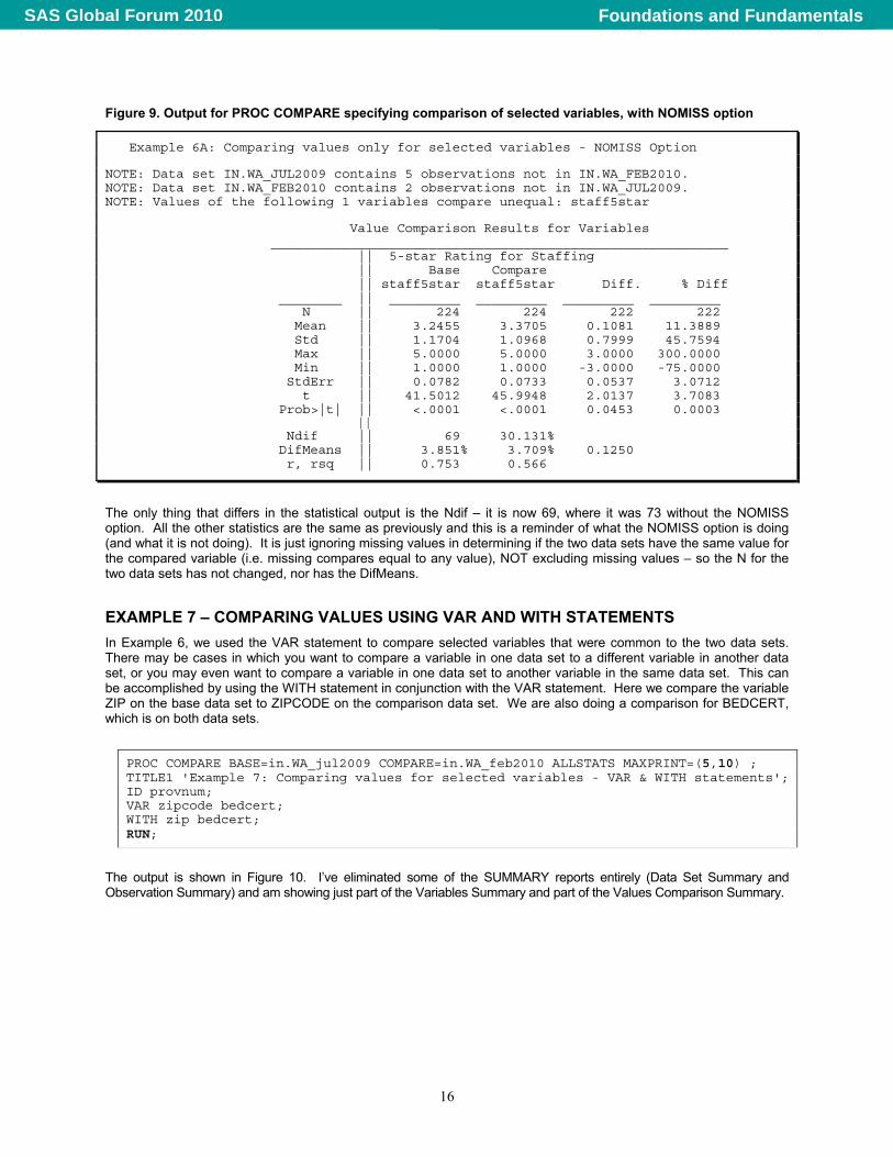
Figure 9. Output for PROC COMPARE specifying comparison of selected variables, with NOMISS option

Example 6A: Comparing values only for selected variables - NOMISS Option NOTE: Data set IN.WA_JUL2009 contains 5 observations not in IN.WA_FEB2010. NOTE: Data set IN.WA_FEB2010 contains 2 observations not in IN.WA_JUL2009. NOTE: Values of the following 1 variables compare unequal: staff5star Value Comparison Results for Variables __________________________________________________________ || 5-star Rating for Staffing || Base Compare || staff5star staff5star Diff. % Diff ________ || _________ _________ _________ _________ N || 224 224 222 222 Mean || 3.2455 3.3705 0.1081 11.3889 Std || 1.1704 1.0968 0.7999 45.7594 Max || 5.0000 5.0000 3.0000 300.0000 Min || 1.0000 1.0000 -3.0000 -75.0000 StdErr || 0.0782 0.0733 0.0537 3.0712 t || 41.5012 45.9948 2.0137 3.7083 Prob>|t| || <.0001 <.0001 0.0453 0.0003 || Ndif || 69 30.131% DifMeans || 3.851% 3.709% 0.1250 r, rsq || 0.753 0.566

The only thing that differs in the statistical output is the Ndif – it is now 69, where it was 73 without the NOMISS option. All the other statistics are the same as previously and this is a reminder of what the NOMISS option is doing (and what it is not doing). It is just ignoring missing values in determining if the two data sets have the same value for the compared variable (i.e. missing compares equal to any value), NOT excluding missing values – so the N for the two data sets has not changed, nor has the DifMeans.

EXAMPLE 7 – COMPARING VALUES USING VAR AND WITH STATEMENTS

In Example 6, we used the VAR statement to compare selected variables that were common to the two data sets. There may be cases in which you want to compare a variable in one data set to a different variable in another data set, or you may even want to compare a variable in one data set to another variable in the same data set. This can be accomplished by using the WITH statement in conjunction with the VAR statement. Here we compare the variable ZIP on the base data set to ZIPCODE on the comparison data set. We are also doing a comparison for BEDCERT, which is on both data sets.

PROC COMPARE BASE=in.WA_jul2009 COMPARE=in.WA_feb2010 ALLSTATS MAXPRINT=(5,10) ; TITLE1 'Example 7: Comparing values for selected variables - VAR & WITH statements'; ID provnum; VAR zipcode bedcert; WITH zip bedcert; RUN;

The output is shown in Figure 10. I’ve eliminated some of the SUMMARY reports entirely (Data Set Summary and Observation Summary) and am showing just part of the Variables Summary and part of the Values Comparison Summary.

16


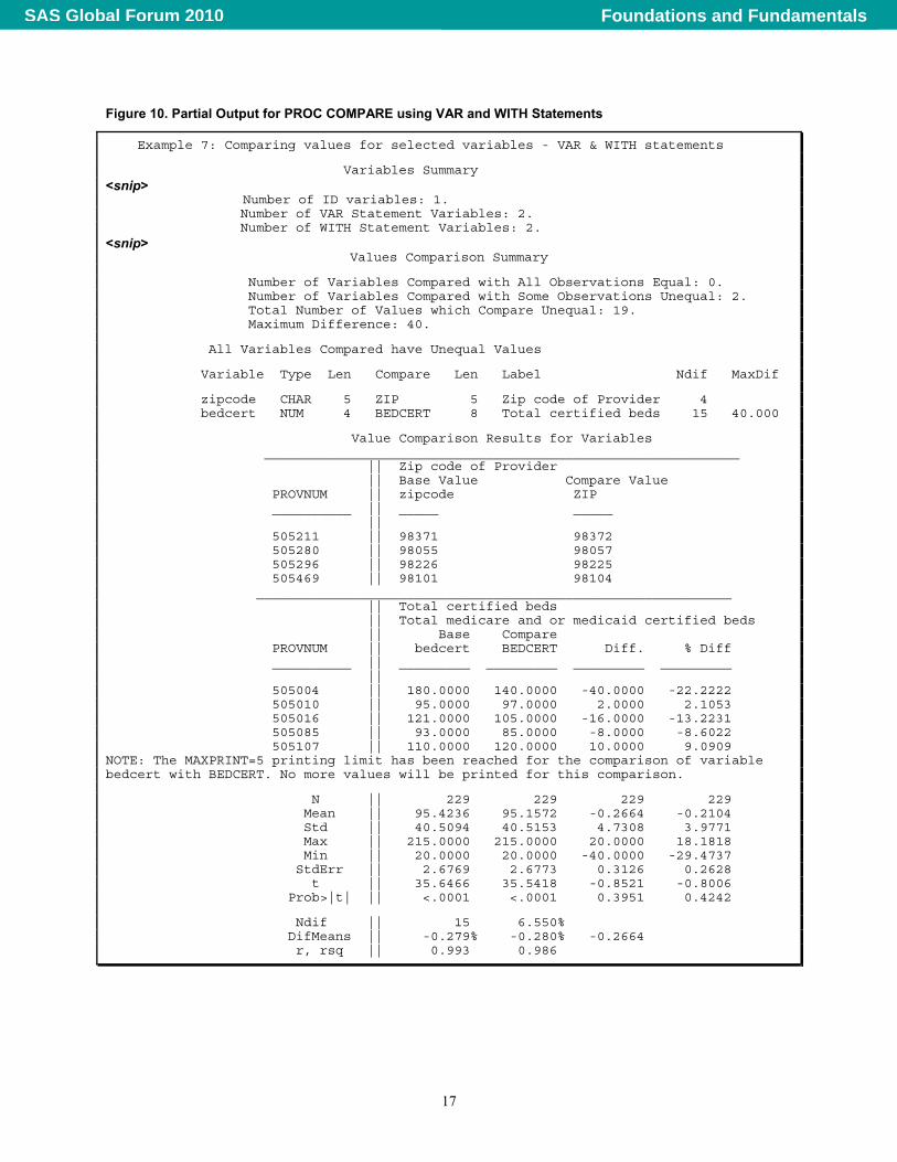
Figure 10. Partial Output for PROC COMPARE using VAR and WITH Statements

Example 7: Comparing values for selected variables - VAR & WITH statements Variables Summary <snip> Number of ID variables: 1. Number of VAR Statement Variables: 2. Number of WITH Statement Variables: 2. <snip>

Values Comparison Summary Number of Variables Compared with All Observations Equal: 0. Number of Variables Compared with Some Observations Unequal: 2. Total Number of Values which Compare Unequal: 19. Maximum Difference: 40. All Variables Compared have Unequal Values Variable Type Len Compare Len Label Ndif MaxDif zipcode CHAR 5 ZIP 5 Zip code of Provider 4 bedcert NUM 4 BEDCERT 8 Total certified beds 15 40.000 Value Comparison Results for Variables ____________________________________________________________ || Zip code of Provider || Base Value Compare Value PROVNUM || zipcode ZIP __________ || _____ _____ || 505211 || 98371 98372 505280 || 98055 98057 505296 || 98226 98225 505469 || 98101 98104 ____________________________________________________________ || Total certified beds || Total medicare and or medicaid certified beds || Base Compare PROVNUM || bedcert BEDCERT Diff. % Diff __________ || _________ _________ _________ _________ || 505004 || 180.0000 140.0000 -40.0000 -22.2222 505010 || 95.0000 97.0000 2.0000 2.1053 505016 || 121.0000 105.0000 -16.0000 -13.2231 505085 || 93.0000 85.0000 -8.0000 -8.6022 505107 || 110.0000 120.0000 10.0000 9.0909 NOTE: The MAXPRINT=5 printing limit has been reached for the comparison of variable bedcert with BEDCERT. No more values will be printed for this comparison. N || 229 229 229 229 Mean || 95.4236 95.1572 -0.2664 -0.2104 Std || 40.5094 40.5153 4.7308 3.9771 Max || 215.0000 215.0000 20.0000 18.1818 Min || 20.0000 20.0000 -40.0000 -29.4737 StdErr || 2.6769 2.6773 0.3126 0.2628 t || 35.6466 35.5418 -0.8521 -0.8006 Prob>|t| || <.0001 <.0001 0.3951 0.4242 Ndif || 15 6.550% DifMeans || -0.279% -0.280% -0.2664 r, rsq || 0.993 0.986

17


A couple of things are of note in the output.

• In the Variables Summary, we see the number of VAR variables and WITH variables.

• In the Values Comparison Summary, we see which variable in the base data set is being compared to which variable in the comparison data set. (Compare this back to what was seen with just the VAR statement – Figure 8.)

• Since ZIP (& ZIPCODE) are character variables, the listing of value comparisons does not include a difference calculation. Similarly, the ALLSTATS option does not produce any output for character variables.

• For the comparison of BEDCERT, there is the same N on both data sets (229) and for the comparison (no missing values on either) so the mean of the differences is identical to the difference in means, namely -0.2664. Recall that this is different than what we saw in Examples 6 and 6A.

• Variables on the VAR and WITH statements are matched up one-to-one; that is, the first variable on the VAR statement in the base data set is compared with the first variable on the WITH statement in the comparison data set, the second with the second, and so on. If the two statements have different numbers of variables the behavior is as follows:

o If there are more variables on the VAR statement than the WITH statement, SAS will try to compare the extra VAR variables in the base data with variables of the same name on the comparison data set.

If such a variable exists, the comparison will occur as if the variable had been included on the WITH statement, though a warning will go into the log stating “WARNING: The WITH statement list is shorter than the VAR statement list.” For example, if BEDCERT had been left off the WITH statement in this example, the output would be identical to that shown in Figure 10.

If such a variable does not exist, then the extra variable(s) on the VAR statement is ignored, but the comparison for the matching variables would proceed. Two warnings are produced. For example, if the variable REVIS_C1 (which is on the July 2009 data set but not the Feb 2010 dataset; Figure xx) was included on the VAR statement, the following warnings would be generated:

WARNING: The WITH statement list is shorter than the VAR statement list. WARNING: The following 1 variables are not in IN.WA_FEB2010: revis_c1.

But the comparison of ZIP and ZIPCODE and BEDCERT with BEDCERT would proceed, producing the same output as in Figure 10.

o If there are more variables on the WITH statement than the VAR statement, SAS will put a WARNING in the log stating “WARNING: The WITH statement list is longer than the VAR statement list” but will then essentially ignore the extra variables on the WITH statement, whether or not these variables exist on the base data set. For example, if BEDCERT was left off the VAR statement, only the comparison of ZIP and ZIPCODE would be generated. And if another variable that existed on just the comparison data set was added on the WITH statement, only the one warning about more variables on the WITH statement would be produced in the log, and the comparison of the matching WITH and VAR variables (here ZIP with ZIPCODE and BEDCERT with BEDCERT) would occur.

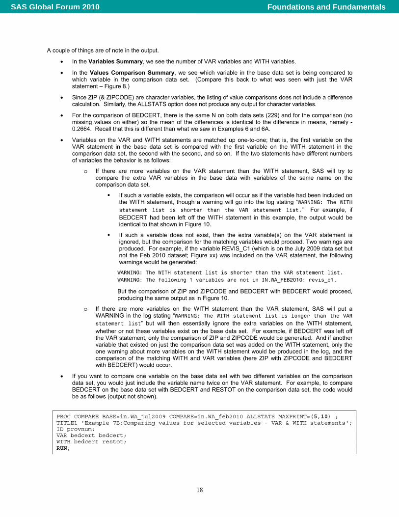
• If you want to compare one variable on the base data set with two different variables on the comparison data set, you would just include the variable name twice on the VAR statement. For example, to compare BEDCERT on the base data set with BEDCERT and RESTOT on the comparison data set, the code would be as follows (output not shown).

PROC COMPARE BASE=in.WA_jul2009 COMPARE=in.WA_feb2010 ALLSTATS MAXPRINT=(5,10) ; TITLE1 'Example 7B:Comparing values for selected variables - VAR & WITH statements'; ID provnum; VAR bedcert bedcert; WITH bedcert restot; RUN;

18


EXAMPLE 8 – COMPARING VARIABLES IN THE SAME DATA SET

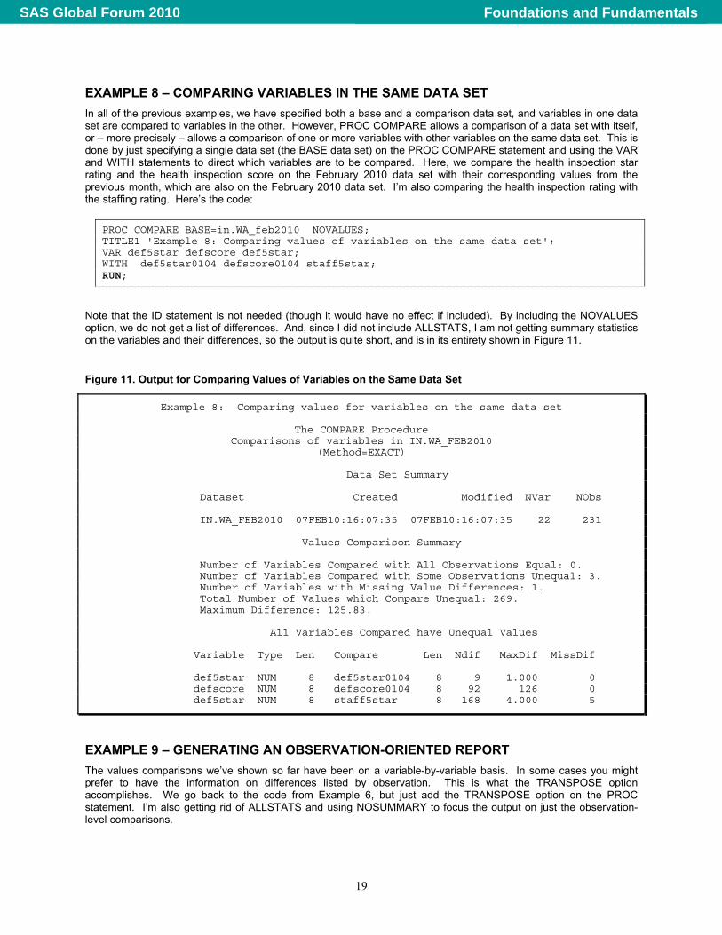
In all of the previous examples, we have specified both a base and a comparison data set, and variables in one data set are compared to variables in the other. However, PROC COMPARE allows a comparison of a data set with itself, or – more precisely – allows a comparison of one or more variables with other variables on the same data set. This is done by just specifying a single data set (the BASE data set) on the PROC COMPARE statement and using the VAR and WITH statements to direct which variables are to be compared. Here, we compare the health inspection star rating and the health inspection score on the February 2010 data set with their corresponding values from the previous month, which are also on the February 2010 data set. I’m also comparing the health inspection rating with the staffing rating. Here’s the code:

PROC COMPARE BASE=in.WA_feb2010 NOVALUES; TITLE1 'Example 8: Comparing values of variables on the same data set'; VAR def5star defscore def5star; WITH def5star0104 defscore0104 staff5star; RUN;

Note that the ID statement is not needed (though it would have no effect if included). By including the NOVALUES option, we do not get a list of differences. And, since I did not include ALLSTATS, I am not getting summary statistics on the variables and their differences, so the output is quite short, and is in its entirety shown in Figure 11.

Figure 11. Output for Comparing Values of Variables on the Same Data Set

Example 8: Comparing values for variables on the same data set

The COMPARE Procedure Comparisons of variables in IN.WA_FEB2010

(Method=EXACT)

Data Set Summary Dataset Created Modified NVar NObs IN.WA_FEB2010 07FEB10:16:07:35 07FEB10:16:07:35 22 231 Values Comparison Summary Number of Variables Compared with All Observations Equal: 0. Number of Variables Compared with Some Observations Unequal: 3. Number of Variables with Missing Value Differences: 1. Total Number of Values which Compare Unequal: 269. Maximum Difference: 125.83. All Variables Compared have Unequal Values Variable Type Len Compare Len Ndif MaxDif MissDif def5star NUM 8 def5star0104 8 9 1.000 0 defscore NUM 8 defscore0104 8 92 126 0 def5star NUM 8 staff5star 8 168 4.000 5

EXAMPLE 9 – GENERATING AN OBSERVATION-ORIENTED REPORT

The values comparisons we’ve shown so far have been on a variable-by-variable basis. In some cases you might prefer to have the information on differences listed by observation. This is what the TRANSPOSE option accomplishes. We go back to the code from Example 6, but just add the TRANSPOSE option on the PROC statement. I’m also getting rid of ALLSTATS and using NOSUMMARY to focus the output on just the observation-level comparisons.

19


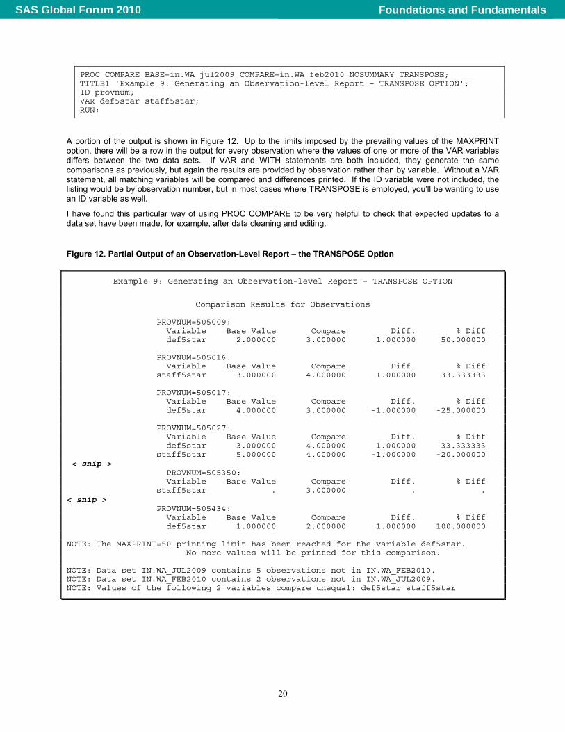
PROC COMPARE BASE=in.WA_jul2009 COMPARE=in.WA_feb2010 NOSUMMARY TRANSPOSE; TITLE1 'Example 9: Generating an Observation-level Report – TRANSPOSE OPTION'; ID provnum; VAR def5star staff5star; RUN;

A portion of the output is shown in Figure 12. Up to the limits imposed by the prevailing values of the MAXPRINT option, there will be a row in the output for every observation where the values of one or more of the VAR variables differs between the two data sets. If VAR and WITH statements are both included, they generate the same comparisons as previously, but again the results are provided by observation rather than by variable. Without a VAR statement, all matching variables will be compared and differences printed. If the ID variable were not included, the listing would be by observation number, but in most cases where TRANSPOSE is employed, you’ll be wanting to use an ID variable as well.

I have found this particular way of using PROC COMPARE to be very helpful to check that expected updates to a data set have been made, for example, after data cleaning and editing.

Figure 12. Partial Output of an Observation-Level Report – the TRANSPOSE Option

Example 9: Generating an Observation-level Report – TRANSPOSE OPTION

Comparison Results for Observations

PROVNUM=505009: Variable Base Value Compare Diff. % Diff def5star 2.000000 3.000000 1.000000 50.000000 PROVNUM=505016: Variable Base Value Compare Diff. % Diff staff5star 3.000000 4.000000 1.000000 33.333333 PROVNUM=505017: Variable Base Value Compare Diff. % Diff def5star 4.000000 3.000000 -1.000000 -25.000000 PROVNUM=505027: Variable Base Value Compare Diff. % Diff def5star 3.000000 4.000000 1.000000 33.333333 staff5star 5.000000 4.000000 -1.000000 -20.000000 < snip > PROVNUM=505350: Variable Base Value Compare Diff. % Diff staff5star . 3.000000 . . < snip > PROVNUM=505434: Variable Base Value Compare Diff. % Diff def5star 1.000000 2.000000 1.000000 100.000000 NOTE: The MAXPRINT=50 printing limit has been reached for the variable def5star. No more values will be printed for this comparison. NOTE: Data set IN.WA_JUL2009 contains 5 observations not in IN.WA_FEB2010. NOTE: Data set IN.WA_FEB2010 contains 2 observations not in IN.WA_JUL2009. NOTE: Values of the following 2 variables compare unequal: def5star staff5star

20


EXAMPLE 10 – GENERATING AN OUTPUT DATA SET OF DIFFERENCES

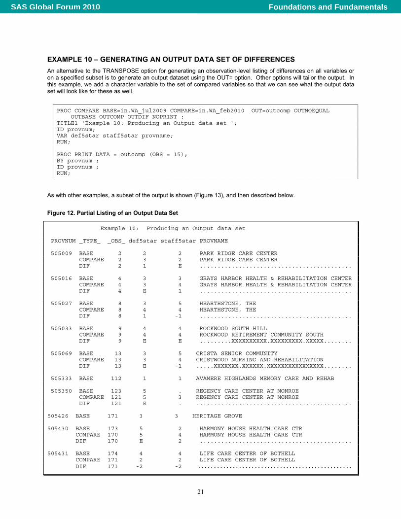
An alternative to the TRANSPOSE option for generating an observation-level listing of differences on all variables or on a specified subset is to generate an output dataset using the OUT= option. Other options will tailor the output. In this example, we add a character variable to the set of compared variables so that we can see what the output data set will look like for these as well.

PROC COMPARE BASE=in.WA_jul2009 COMPARE=in.WA_feb2010 OUT=outcomp OUTNOEQUAL OUTBASE OUTCOMP OUTDIF NOPRINT ;

TITLE1 'Example 10: Producing an Output data set '; ID provnum; VAR def5star staff5star provname; RUN; PROC PRINT DATA = outcomp (OBS = 15); BY provnum ; ID provnum ; RUN;

As with other examples, a subset of the output is shown (Figure 13), and then described below.

Figure 12. Partial Listing of an Output Data Set

Example 10: Producing an Output data set PROVNUM _TYPE_ _OBS_ def5star staff5star PROVNAME 505009 BASE 2 2 2 PARK RIDGE CARE CENTER COMPARE 2 3 2 PARK RIDGE CARE CENTER DIF 2 1 E ........................................... 505016 BASE 4 3 3 GRAYS HARBOR HEALTH & REHABILITATION CENTER COMPARE 4 3 4 GRAYS HARBOR HEALTH & REHABILITATION CENTER DIF 4 E 1 ........................................... 505027 BASE 8 3 5 HEARTHSTONE, THE COMPARE 8 4 4 HEARTHSTONE, THE DIF 8 1 -1 ........................................... 505033 BASE 9 4 4 ROCKWOOD SOUTH HILL COMPARE 9 4 4 ROCKWOOD RETIREMENT COMMUNITY SOUTH DIF 9 E E .........XXXXXXXXXX.XXXXXXXXX.XXXXX........ 505069 BASE 13 3 5 CRISTA SENIOR COMMUNITY COMPARE 13 3 4 CRISTWOOD NURSING AND REHABILITATION DIF 13 E -1 .....XXXXXXX.XXXXXX.XXXXXXXXXXXXXXXX........ 505333 BASE 112 1 1 AVAMERE HIGHLANDS MEMORY CARE AND REHAB 505350 BASE 123 5 . REGENCY CARE CENTER AT MONROE COMPARE 121 5 3 REGENCY CARE CENTER AT MONROE DIF 121 E . ............................................ 505426 BASE 171 3 3 HERITAGE GROVE 505430 BASE 173 5 2 HARMONY HOUSE HEALTH CARE CTR COMPARE 170 5 4 HARMONY HOUSE HEALTH CARE CTR DIF 170 E 2 ........................................... 505431 BASE 174 4 4 LIFE CARE CENTER OF BOTHELL COMPARE 171 2 2 LIFE CARE CENTER OF BOTHELL DIF 171 -2 -2 .................................................

21


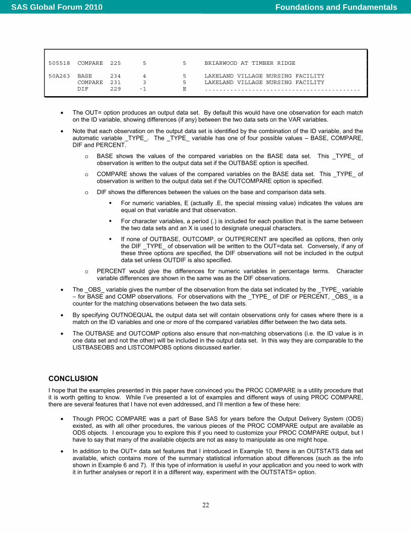
505518 COMPARE 225 5 5 BRIARWOOD AT TIMBER RIDGE 50A263 BASE 234 4 5 LAKELAND VILLAGE NURSING FACILITY COMPARE 231 3 5 LAKELAND VILLAGE NURSING FACILITY DIF 229 -1 E ...........................................

• The OUT= option produces an output data set. By default this would have one observation for each match on the ID variable, showing differences (if any) between the two data sets on the VAR variables.

• Note that each observation on the output data set is identified by the combination of the ID variable, and the automatic variable _TYPE_. The _TYPE_ variable has one of four possible values – BASE, COMPARE, DIF and PERCENT.

o BASE shows the values of the compared variables on the BASE data set. This _TYPE_ of observation is written to the output data set if the OUTBASE option is specified.

o COMPARE shows the values of the compared variables on the BASE data set. This _TYPE_ of observation is written to the output data set if the OUTCOMPARE option is specified.

o DIF shows the differences between the values on the base and comparison data sets.

For numeric variables, E (actually .E, the special missing value) indicates the values are equal on that variable and that observation.

For character variables, a period (.) is included for each position that is the same between the two data sets and an X is used to designate unequal characters.

If none of OUTBASE, OUTCOMP, or OUTPERCENT are specified as options, then only the DIF _TYPE_ of observation will be written to the OUT=data set. Conversely, if any of these three options are specified, the DIF observations will not be included in the output data set unless OUTDIF is also specified.

o PERCENT would give the differences for numeric variables in percentage terms. Character variable differences are shown in the same was as the DIF observations.

• The _OBS_ variable gives the number of the observation from the data set indicated by the _TYPE_ variable – for BASE and COMP observations. For observations with the _TYPE_ of DIF or PERCENT, _OBS_ is a counter for the matching observations between the two data sets.

• By specifying OUTNOEQUAL the output data set will contain observations only for cases where there is a match on the ID variables and one or more of the compared variables differ between the two data sets.

• The OUTBASE and OUTCOMP options also ensure that non-matching observations (i.e. the ID value is in one data set and not the other) will be included in the output data set. In this way they are comparable to the LISTBASEOBS and LISTCOMPOBS options discussed earlier.

CONCLUSION

I hope that the examples presented in this paper have convinced you the PROC COMPARE is a utility procedure that it is worth getting to know. While I’ve presented a lot of examples and different ways of using PROC COMPARE, there are several features that I have not even addressed, and I’ll mention a few of these here:

• Though PROC COMPARE was a part of Base SAS for years before the Output Delivery System (ODS) existed, as with all other procedures, the various pieces of the PROC COMPARE output are available as ODS objects. I encourage you to explore this if you need to customize your PROC COMPARE output, but I have to say that many of the available objects are not as easy to manipulate as one might hope.

• In addition to the OUT= data set features that I introduced in Example 10, there is an OUTSTATS data set available, which contains more of the summary statistical information about differences (such as the info shown in Example 6 and 7). If this type of information is useful in your application and you need to work with it in further analyses or report it in a different way, experiment with the OUTSTATS= option.

22


23

• PROC COMPARE has a BY statement, which allows you to stratify your comparison on variables of interest. This works pretty much the way the BY statement works in other procedures, and would provide a way of examining whether data set differences vary in systematic ways based on stratification (BY) variables of interest.

• While I discussed the CRITERION and METHOD options briefly, if your COMPARE needs are such that you need to control what is meant by “equality”, you’ll need to work with these options further to fine tune your comparisons. Additionally, there is a FUZZ= option that can be used to control what differences are printed.

• When PROC COMPARE runs, a return code is stored in the automatic macro variable SYSINFO, and the value of this code provides information about the comparison results. For example, there are different values for minor differences such as the data sets have differing labels vs. potentially more critical differences such as conflicting variable types or value differences. The values are scaled so that these types of differences could be parsed from the SYSINFO variable, potentially to direct further processing. There is a table of these values in the PROC COMPARE chapter of the Base SAS Procedures guide, referenced below.

I’ve found this PROC to be really useful in a lot of my work with big government data sets – just another way to get to know your data. If you’ve never used it – or it has been a while, take another look. And, happy COMPARE-ing!

REFERENCES

SAS Institute Inc. 2009. The COMPARE Procedure. Base SAS® 9.2 Procedures Guide. Cary, NC: SAS Institute Inc.

CONTACT INFORMATION

Your comments and questions are valued and encouraged. Contact the author at:

Name: Christianna Williams Enterprise: Abt Associates Inc. E-mail: [email protected]

SAS and all other SAS Institute Inc. product or service names are registered trademarks or trademarks of SAS Institute Inc. in the USA and other countries. ® indicates USA registration.

Other brand and product names are trademarks of their respective companies.


mailto:[email protected]

Documents

149-2010: PROC COMPARE: Worth Another Look!support.sas.com/resources/papers/proceedings10/149-2010.pdf · PROC COMPARE – Worth Another Look! Christianna S. Williams, Abt Associates