Embed Size (px)
Citation preview
15. GEOMETRY AND COORDINATES
We define . Given we say that the x-coordinate is while the y-
coordinate is . We can view the coordinates as mappings from to :
Coordinates take in a point in the plane and output a real number.
Polar coordinates are based on partitioning the plane into circles or rays from the origin. Each point in
the plane will be found on a unique circle and ray hence we can label the point by the radius of the
circle and the angle of the ray. Some ambiguity arises in assigning the angle because there is a natural
duplicity in the assignment. We can always add an integer multiple of 360 degrees or radians. This
means if we are to be open minded about angles then we have to accept there is more than one correct
answer to a given question. Once the basics of polar coordinates are complete we study parametric
curves and the calculation of areas and arclength in polar coordinates (currently there are no examples
or discussion of area or arclength in polars, see Section 11.4 of Stewart for examples, I will probably
work additional examples in lecture).
Another major topic in geometry is that of conic sections. We review the major equations and the
geometric definitions which define the ellipse, parabola and hyperbola. If time permits we may also
examine the polar form of their equations in lecture (although it is not found in these notes presently)
Finally, I conclude this chapter by exploring the existence of other coordinate systems in the plane.
Modern calculus texts have little if anything to say about the general concept of coordinates. I try to give
you some idea of how we invent coordinates in the conclusion of this chapter. By the way, the concept
of a coordinate system in physics is a bit more general. I would say that a coordinate system in physics is
an “observer”. An “observer” is a mapping from to the space of all coordinates on . At each time
we get a different coordinate system, the origin for an observer can move. I describe these ideas
carefully in my ma430 notes. Let me just say for conceptual clarity that our coordinate systems are fixed
and immovable.
15.1. POLAR COORDINATES
Polar coordinates are denoted . If we wanted polar coordinates to be uniquely defined we
could insist that and . However, we will allow hence the polar
coordinates are not uniquely defined. Many different angles will describe the same direction
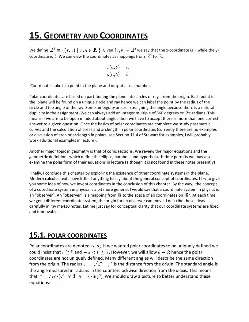
from the origin. The radius is the distance from the origin. The standard angle is
the angle measured in radians in the counterclockwise direction from the x-axis. This means
that . We should draw a picture to better understand these
equations:
You may recall that calculation of the standard angle requires some care. While it is true that
for all points with it is not true that in general. In quadrants II
and III the inverse tangent formula fails. You must think about this.
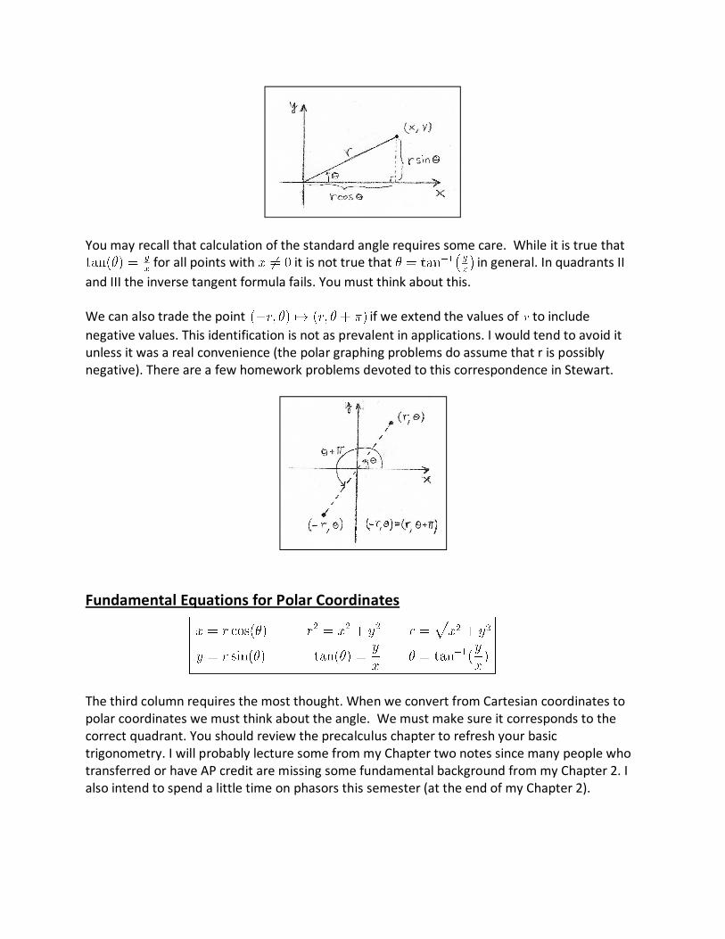
We can also trade the point if we extend the values of to include
negative values. This identification is not as prevalent in applications. I would tend to avoid it
unless it was a real convenience (the polar graphing problems do assume that r is possibly
negative). There are a few homework problems devoted to this correspondence in Stewart.
Fundamental Equations for Polar Coordinates
The third column requires the most thought. When we convert from Cartesian coordinates to
polar coordinates we must think about the angle. We must make sure it corresponds to the
correct quadrant. You should review the precalculus chapter to refresh your basic
trigonometry. I will probably lecture some from my Chapter two notes since many people who
transferred or have AP credit are missing some fundamental background from my Chapter 2. I
also intend to spend a little time on phasors this semester (at the end of my Chapter 2).
Example 15.1.1
Find the polar coordinates for the point (1,1).
If tangent is one that means , in quadrant I we find solution . Hence the
polar coordinates of this point are
Example 15.1.2
Find the polar coordinates for the point .
The given point is in quadrant II thus we find . Hence the polar coordinates of
this point are
Graphing with polar coordinates:
The goal for rest of this section is to get a feel for how to graph in polar coordinates. We work a
few purely polar problems. We also try translating a few standard Cartesian graphs. The general
story is that both polar and Cartesian coordinates have their own respective virtues. Broadly
speaking, polar coordinates help simplify equations of circles while Cartesian coordinates make
equations of lines particularly nice.
Example 15.1.3
Find the equation of the line in polar coordinates. We simply substitute the
transformation equations to obtain:
We don’t need to solve for the radius necessarily. I like to solve for it when I can since it’s easy
to think about constructing the graph. Logically the angle is just as primary. In the same sense it
is essentially a matter of habit and convenience that we almost always solve for y in the
Cartesian coordinates.
Remark: one important strategy to graph polar graphs is to first plot the radius as a function of
the standard angle in a separate graph. Then you can use that to create the graph in the xy-
plane. We will examine this approach in lecture, it is not emphasized in these notes . It’s easier
to see on the white board since it involves drawing one graph and then extrapolating to draw a
second graph. Examples 7 and 8 of Section 11.3 of Stewart illustrate this approach. My
approach is primarily algebraic in these notes, but in practice I would advocate a mixture of
algebraic reasoning and CAS-aided visualization.
Example 15.1.4
Consider the polar equation . Find the equivalent Cartesian equation:
This is a circle of radius two centered at the origin.
Example 15.1.5
If then what is the corresponding polar equation? Substitute as usual,
When the circle is not centered at the origin the equation for the circle in polar coordinates will
involve the standard angle in a non-trivial manner.
Example 15.1.6
What is the Cartesian equation that is equivalent to ? We have two equations:
We eliminate the radius by dividing the equations above:
To be careful I should emphasize this is only valid in quadrant I. The other half of the line goes
with . In other words, the graph of is a ray based at the origin. It would be the
whole line if we allowed for negative radius.
Remark: if we fix the standard angle to be some constant we have seen it gives us a ray from
the origin. If we set the radius to be some constant we obtain a circle. Contrast this to the
Cartesian case; is a vertical line, is a horizontal line.
In-class Exercise 15.1.7
Graph . Make a table of values to begin then use an algebraic argument to verify
your suspicion about the identity of this curve.
Not all polar curves correspond to known Cartesian curves. Sometimes we just have to make a
table of values and graph by connecting the dots, or Mathematica.
In-class Exercise 15.1.8
Graph . Consider using a graph in the -plane to generate the graph of the given
curve in the xy-plane. (Stewart calls the -plane “Cartesian coordinates” , see Fig. 10 or 12 on
page 679)
I suppose it took all of us a number of examples before we really understood Cartesian
coordinates. The same is true for other coordinate systems. Your homework explores a few
more examples that will hopefully help you better understand polar coordinates.
Polar Form of Complex Numbers Recall that we learned a complex number corresponds to the point . What are
the polar coordinates of that point and how does the imaginary exponential come into play
here? Observe,
The calculation above justifies the assertion that a complex number may be put into its polar
form. In particular we define,
Much can be said here, but we leave that discussion for the complex variables course. If this
interests you I have a book which is quite readable on the subject. Just ask.
In-class Exercise 15.1.10
Find the polar form of the complex number . Find the polar form of the complex
number . Find the polar form of the complex number . Graph both and in the
complex plane. How are the points related?
Remark: In electrical engineering complex numbers are used to model the impedance The
neat thing is that AC-circuits can be treated as DC-circuits if the voltage source is sinusoidal.
This is called the Phasor method. In short, resistances give real impedance while capacitors and
inductors give purely imaginary impedance. The net impedance for a circuit is generally
complex.
Remark: there is much more to read in my Chapter 2, go read my Section 2.9.
Definition 15.1.9: (Polar Form of Complex Number) Let the polar form
of is where and is the standard angle of .
15.2: Parametric Curves in Polar Coordinates Same idea as we have discussed thus far for Cartesian coordinates, except now we need a
parametric equation for .
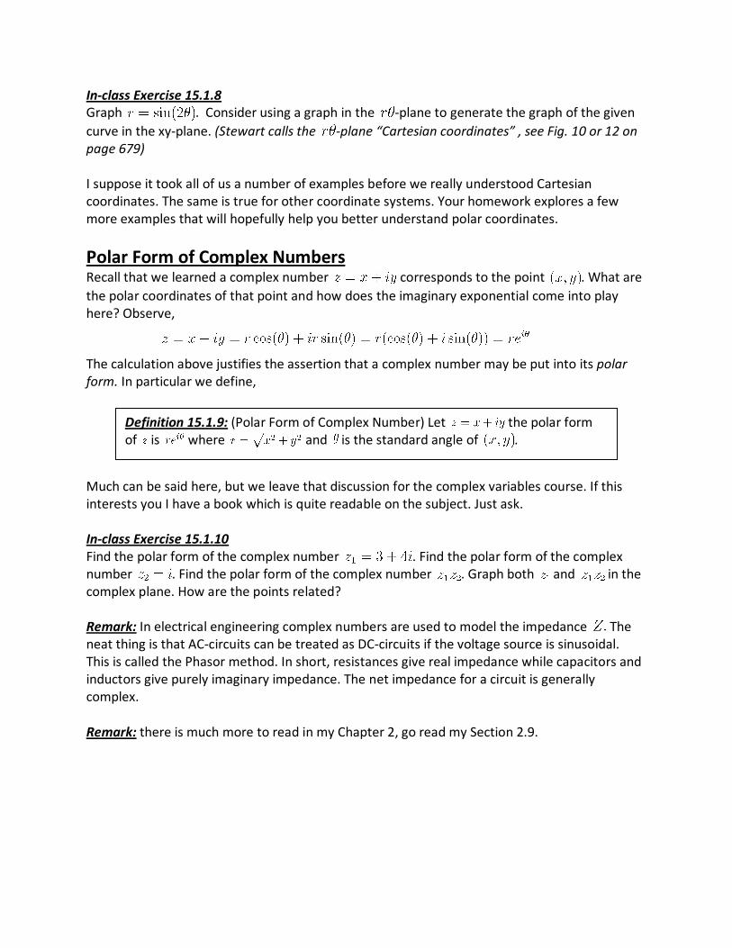
Example 15.2.1: Describe the curve given by the parametric equations for
. We can make a table of values to helps graph the curve,
Example 15.2.2: Describe the curve given by the parametric equations for
. This is spiral goes inward,
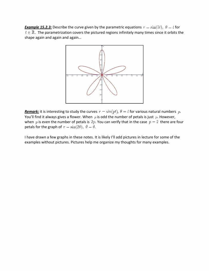
Example 15.2.3: Describe the curve given by the parametric equations for
. The parametrization covers the pictured regions infinitely many times since it orbits the
shape again and again and again…
Remark: it is interesting to study the curves , for various natural numbers .
You’ll find it always gives a flower. When is odd the number of petals is just . However,
when is even the number of petals is . You can verify that in the case there are four
petals for the graph of .
I have drawn a few graphs in these notes. It is likely I’ll add pictures in lecture for some of the
examples without pictures. Pictures help me organize my thoughts for many examples.
15.3. CONIC SECTIONS
Take a look in Stewart, he has a nice picture of how a cone can be sliced by a plane to give a
parabola, hyperbola or an ellipse. Let me remind you the basic definitions and canonical
(standard) formulae for the conic sections. I have saved the task of deriving the formula from
the geometric definition for homework. Each derivation is a good algebra exercise, and they can
be found in many text books.
Proof: see Stewart.
There are similar equations for parabolas built from a vertical directerix. If you understand this
equation it is a simple matter to twist it to get the sideways parabola equation.
Proof: see Stewart.
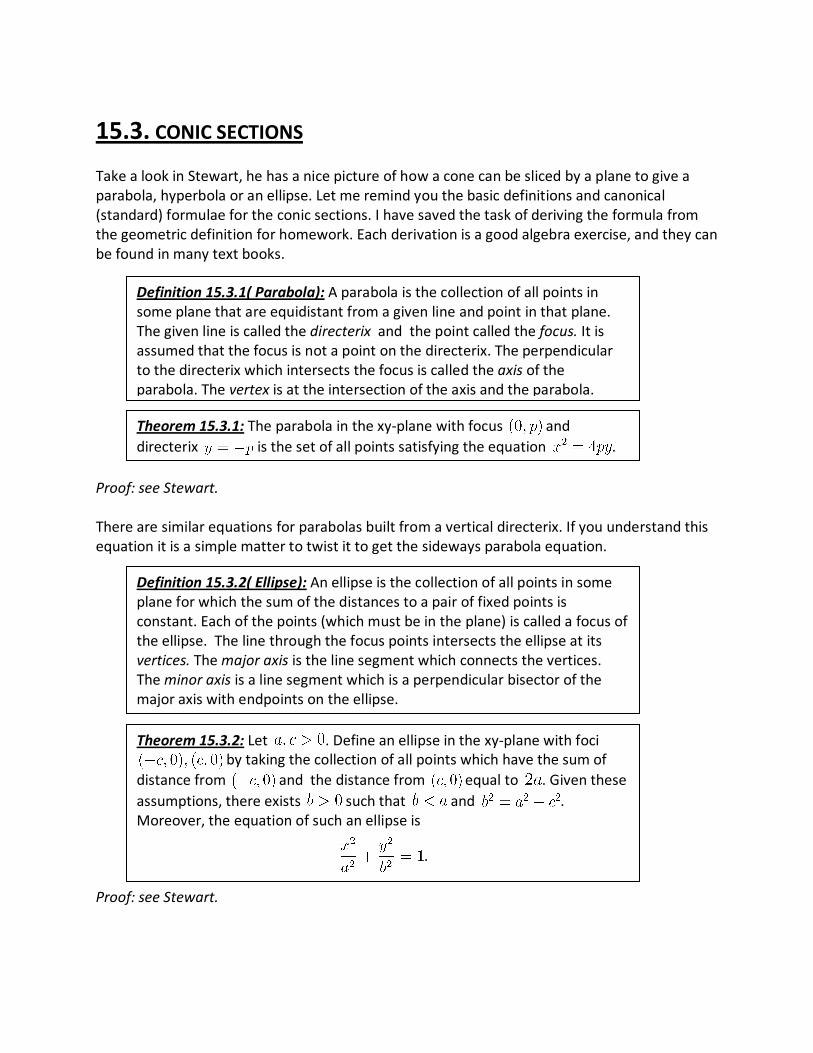
Definition 15.3.1( Parabola): A parabola is the collection of all points in
some plane that are equidistant from a given line and point in that plane.
The given line is called the directerix and the point called the focus. It is
assumed that the focus is not a point on the directerix. The perpendicular
to the directerix which intersects the focus is called the axis of the
parabola. The vertex is at the intersection of the axis and the parabola.
Definition 15.3.2( Ellipse): An ellipse is the collection of all points in some
plane for which the sum of the distances to a pair of fixed points is
constant. Each of the points (which must be in the plane) is called a focus of
the ellipse. The line through the focus points intersects the ellipse at its
vertices. The major axis is the line segment which connects the vertices.
The minor axis is a line segment which is a perpendicular bisector of the
major axis with endpoints on the ellipse.
Theorem 15.3.2: Let . Define an ellipse in the xy-plane with foci
by taking the collection of all points which have the sum of
distance from and the distance from equal to . Given these
assumptions, there exists such that and .
Moreover, the equation of such an ellipse is
.
Theorem 15.3.1: The parabola in the xy-plane with focus and
directerix is the set of all points satisfying the equation .
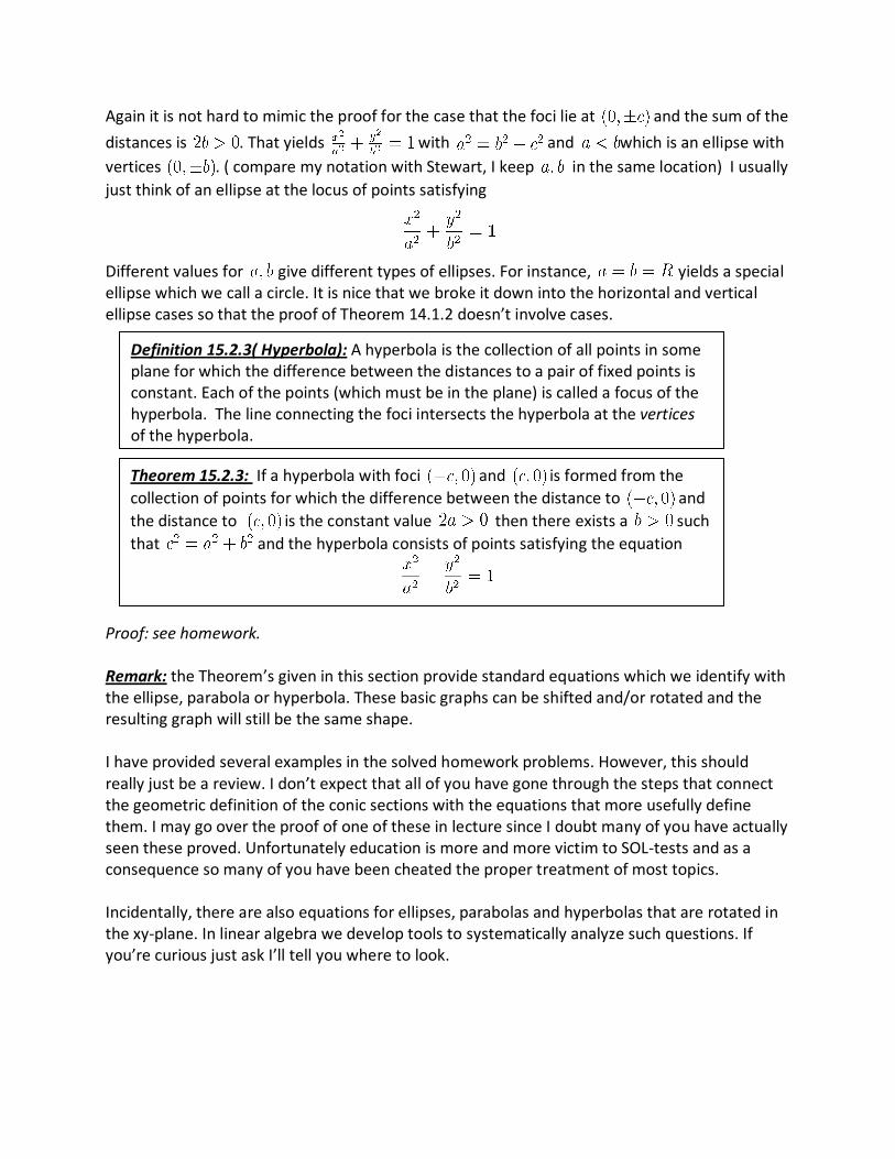
Again it is not hard to mimic the proof for the case that the foci lie at and the sum of the
distances is . That yields with and which is an ellipse with
vertices . ( compare my notation with Stewart, I keep in the same location) I usually
just think of an ellipse at the locus of points satisfying
Different values for give different types of ellipses. For instance, yields a special
ellipse which we call a circle. It is nice that we broke it down into the horizontal and vertical
ellipse cases so that the proof of Theorem 14.1.2 doesn’t involve cases.
Proof: see homework.
Remark: the Theorem’s given in this section provide standard equations which we identify with
the ellipse, parabola or hyperbola. These basic graphs can be shifted and/or rotated and the
resulting graph will still be the same shape.
I have provided several examples in the solved homework problems. However, this should
really just be a review. I don’t expect that all of you have gone through the steps that connect
the geometric definition of the conic sections with the equations that more usefully define
them. I may go over the proof of one of these in lecture since I doubt many of you have actually
seen these proved. Unfortunately education is more and more victim to SOL-tests and as a
consequence so many of you have been cheated the proper treatment of most topics.
Incidentally, there are also equations for ellipses, parabolas and hyperbolas that are rotated in
the xy-plane. In linear algebra we develop tools to systematically analyze such questions. If
you’re curious just ask I’ll tell you where to look.
Theorem 15.2.3: If a hyperbola with foci and is formed from the
collection of points for which the difference between the distance to and
the distance to is the constant value then there exists a such
that and the hyperbola consists of points satisfying the equation
Definition 15.2.3( Hyperbola): A hyperbola is the collection of all points in some
plane for which the difference between the distances to a pair of fixed points is
constant. Each of the points (which must be in the plane) is called a focus of the
hyperbola. The line connecting the foci intersects the hyperbola at the vertices
of the hyperbola.
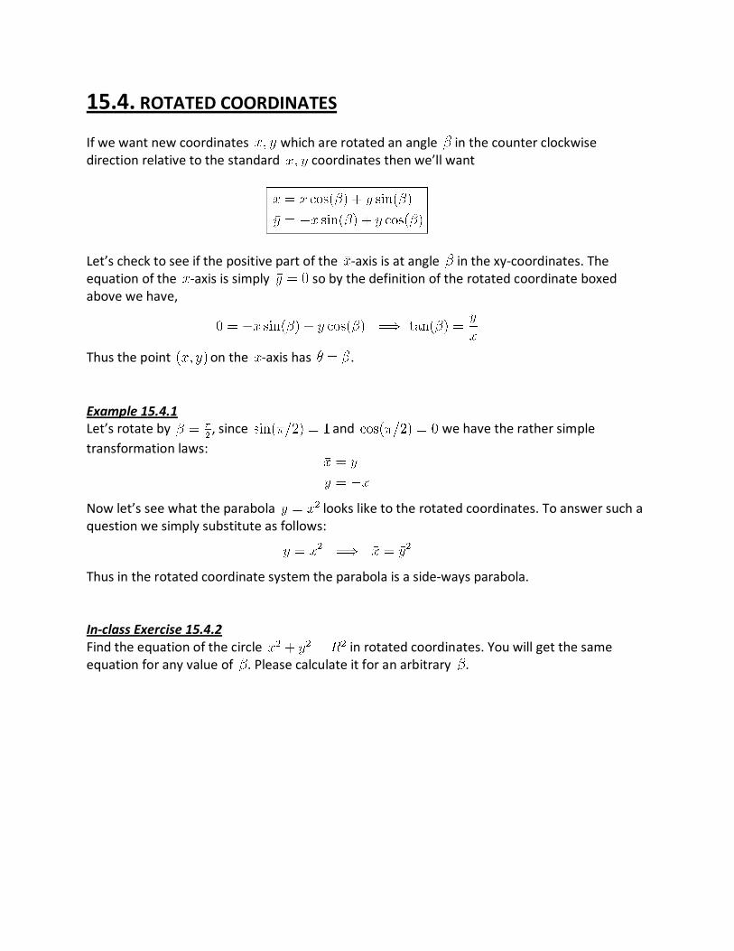
15.4. ROTATED COORDINATES
If we want new coordinates which are rotated an angle in the counter clockwise
direction relative to the standard coordinates then we’ll want
Let’s check to see if the positive part of the -axis is at angle in the xy-coordinates. The
equation of the -axis is simply so by the definition of the rotated coordinate boxed
above we have,
Thus the point on the -axis has .
Example 15.4.1
Let’s rotate by , since and we have the rather simple
transformation laws:
Now let’s see what the parabola looks like to the rotated coordinates. To answer such a
question we simply substitute as follows:
Thus in the rotated coordinate system the parabola is a side-ways parabola.
In-class Exercise 15.4.2
Find the equation of the circle in rotated coordinates. You will get the same
equation for any value of . Please calculate it for an arbitrary .
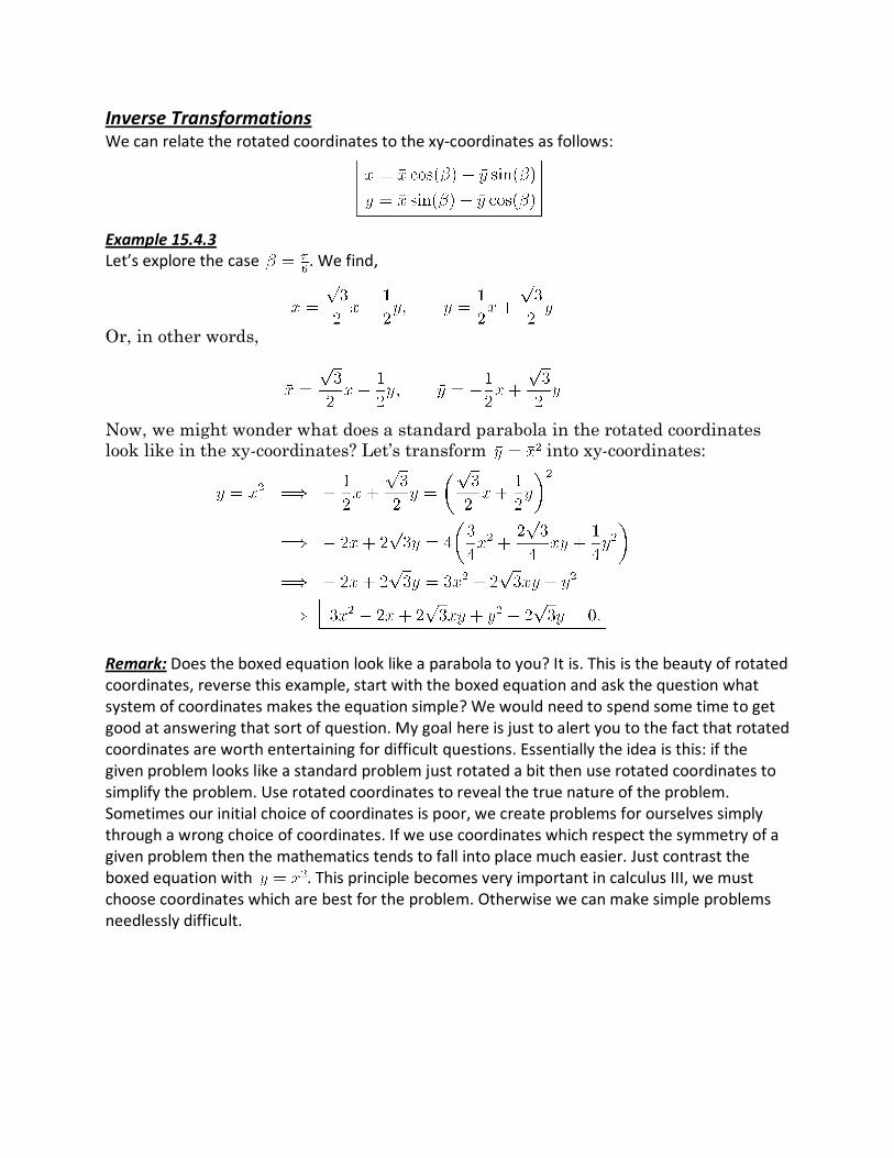
Inverse Transformations
We can relate the rotated coordinates to the xy-coordinates as follows:
Example 15.4.3
Let’s explore the case . We find,
Or, in other words,
Now, we might wonder what does a standard parabola in the rotated coordinates
look like in the xy-coordinates? Let’s transform into xy-coordinates:
Remark: Does the boxed equation look like a parabola to you? It is. This is the beauty of rotated
coordinates, reverse this example, start with the boxed equation and ask the question what
system of coordinates makes the equation simple? We would need to spend some time to get
good at answering that sort of question. My goal here is just to alert you to the fact that rotated
coordinates are worth entertaining for difficult questions. Essentially the idea is this: if the
given problem looks like a standard problem just rotated a bit then use rotated coordinates to
simplify the problem. Use rotated coordinates to reveal the true nature of the problem.
Sometimes our initial choice of coordinates is poor, we create problems for ourselves simply
through a wrong choice of coordinates. If we use coordinates which respect the symmetry of a
given problem then the mathematics tends to fall into place much easier. Just contrast the
boxed equation with . This principle becomes very important in calculus III, we must
choose coordinates which are best for the problem. Otherwise we can make simple problems
needlessly difficult.
15.5. OTHER COORDINATE SYSTEMS This section looks at a variety of non-standard coordinate systems.
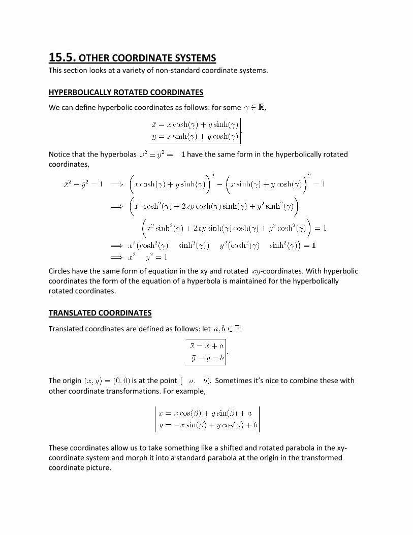
HYPERBOLICALLY ROTATED COORDINATES
We can define hyperbolic coordinates as follows: for some ,
Notice that the hyperbolas have the same form in the hyperbolically rotated
coordinates,
Circles have the same form of equation in the xy and rotated -coordinates. With hyperbolic
coordinates the form of the equation of a hyperbola is maintained for the hyperbolically
rotated coordinates.
TRANSLATED COORDINATES
Translated coordinates are defined as follows: let
.
The origin is at the point . Sometimes it’s nice to combine these with
other coordinate transformations. For example,
These coordinates allow us to take something like a shifted and rotated parabola in the xy-
coordinate system and morph it into a standard parabola at the origin in the transformed
coordinate picture.
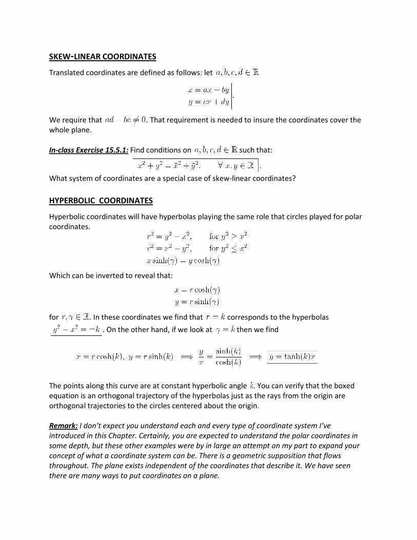
SKEW-LINEAR COORDINATES
Translated coordinates are defined as follows: let
.
We require that . That requirement is needed to insure the coordinates cover the
whole plane.
In-class Exercise 15.5.1: Find conditions on such that:
.
What system of coordinates are a special case of skew-linear coordinates?
HYPERBOLIC COORDINATES
Hyperbolic coordinates will have hyperbolas playing the same role that circles played for polar
coordinates.
Which can be inverted to reveal that:
for . In these coordinates we find that corresponds to the hyperbolas
. On the other hand, if we look at then we find
The points along this curve are at constant hyperbolic angle . You can verify that the boxed
equation is an orthogonal trajectory of the hyperbolas just as the rays from the origin are
orthogonal trajectories to the circles centered about the origin.
Remark: I don’t expect you understand each and every type of coordinate system I’ve
introduced in this Chapter. Certainly, you are expected to understand the polar coordinates in
some depth, but these other examples were by in large an attempt on my part to expand your
concept of what a coordinate system can be. There is a geometric supposition that flows
throughout. The plane exists independent of the coordinates that describe it. We have seen
there are many ways to put coordinates on a plane.
Coordinate Maps on a Surface (a window on higher math)
In abstract manifold theory we find it necessary to refine our concept of a coordinate mapping
to fit the following rather technical prescription. The coordinates discussed in this chapter don’t
quite make the grade. We realize certain coordinates are not one-one. There are multiple
values of the coordinate which map to the same point on the surface. Also, we have not even
begun to worry about smoothness. We need tools from calculus III to tackle that question and
even then this topic is a bit beyond calculus III.
Let be a surface. In fact, let be a two-dimensional manifold. What this means is that there
is a family of open sets for which cover . For each one of these
open sets there exists a one-one mapping which is called a
coordinate map. These coordinate maps must be compatible. This means
is a smooth mapping on .
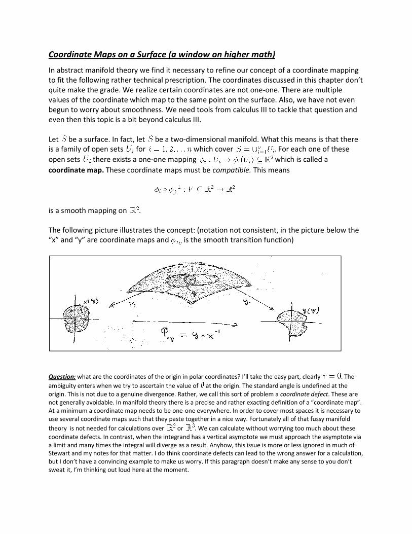
The following picture illustrates the concept: (notation not consistent, in the picture below the
“x” and “y” are coordinate maps and is the smooth transition function)
Question: what are the coordinates of the origin in polar coordinates? I’ll take the easy part, clearly . The
ambiguity enters when we try to ascertain the value of at the origin. The standard angle is undefined at the
origin. This is not due to a genuine divergence. Rather, we call this sort of problem a coordinate defect. These are
not generally avoidable. In manifold theory there is a precise and rather exacting definition of a “coordinate map”.
At a minimum a coordinate map needs to be one-one everywhere. In order to cover most spaces it is necessary to
use several coordinate maps such that they paste together in a nice way. Fortunately all of that fussy manifold
theory is not needed for calculations over or . We can calculate without worrying too much about these
coordinate defects. In contrast, when the integrand has a vertical asymptote we must approach the asymptote via
a limit and many times the integral will diverge as a result. Anyhow, this issue is more or less ignored in much of
Stewart and my notes for that matter. I do think coordinate defects can lead to the wrong answer for a calculation,
but I don’t have a convincing example to make us worry. If this paragraph doesn’t make any sense to you don’t
sweat it, I’m thinking out loud here at the moment.

![Vector Calculus & General Coordinate Systems Orthogonal curvilinear coordinates For orthogonal curvilinear coordinates, recall, Vector Calculus & General Coordinate Systems [, ]](https://img.pdfslide.net/doc/110x75/5b0d24927f8b9a8b038d43de/vector-calculus-general-coordinate-systems-orthogonal-curvilinear-coordinates-for.jpg)