Intro to Database Systems

15-445/15-645

Fall 2020

Andy PavloComputer Science Carnegie Mellon UniversityAP

15 Query PlanningPart II

15-445/645 (Fall 2020)

HAIRCUT

2

15-445/645 (Fall 2020)

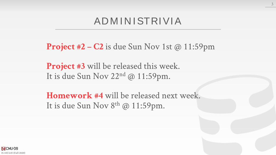
ADMINISTRIVIA

Project #2 – C2 is due Sun Nov 1st @ 11:59pm

Project #3 will be released this week.It is due Sun Nov 22nd @ 11:59pm.

Homework #4 will be released next week.It is due Sun Nov 8th @ 11:59pm.

3

15-445/645 (Fall 2020)

UPCOMING DATABASE TALKS

Datometry→ Monday Oct 26th @ 5pm ET

MySQL Query Optimizer→ Monday Nov 2nd @ 5pm ET

EraDB "Magical Indexes"→ Monday Nov 9th @ 5pm ET

4

15-445/645 (Fall 2020)

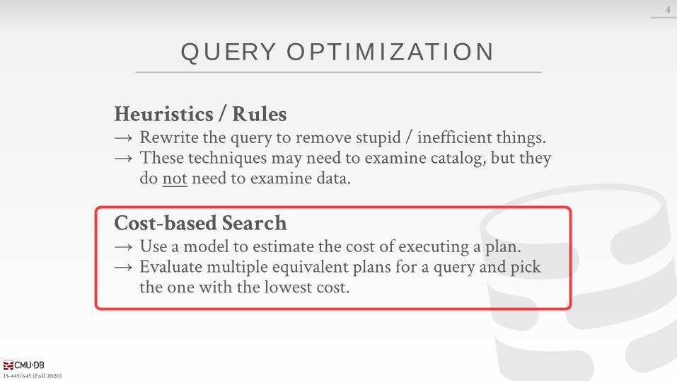
QUERY OPTIMIZATION

Heuristics / Rules→ Rewrite the query to remove stupid / inefficient things.→ These techniques may need to examine catalog, but they

do not need to examine data.

Cost-based Search→ Use a model to estimate the cost of executing a plan.→ Evaluate multiple equivalent plans for a query and pick

the one with the lowest cost.

4

15-445/645 (Fall 2020)

TODAY'S AGENDA

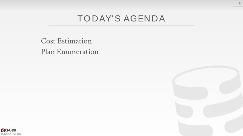
Cost Estimation

Plan Enumeration

5

15-445/645 (Fall 2020)

COST-BASED QUERY PL ANNING

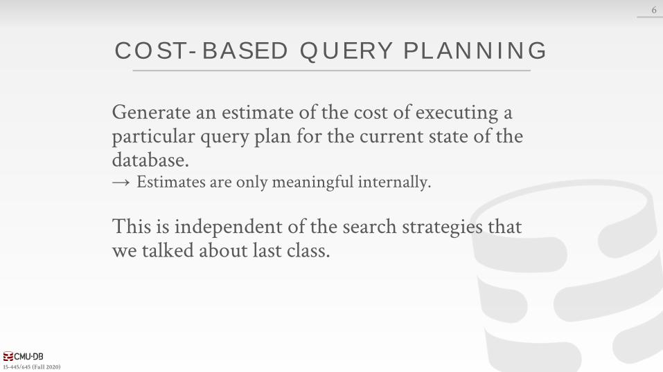
Generate an estimate of the cost of executing a particular query plan for the current state of the database.→ Estimates are only meaningful internally.

This is independent of the search strategies that we talked about last class.

6

15-445/645 (Fall 2020)

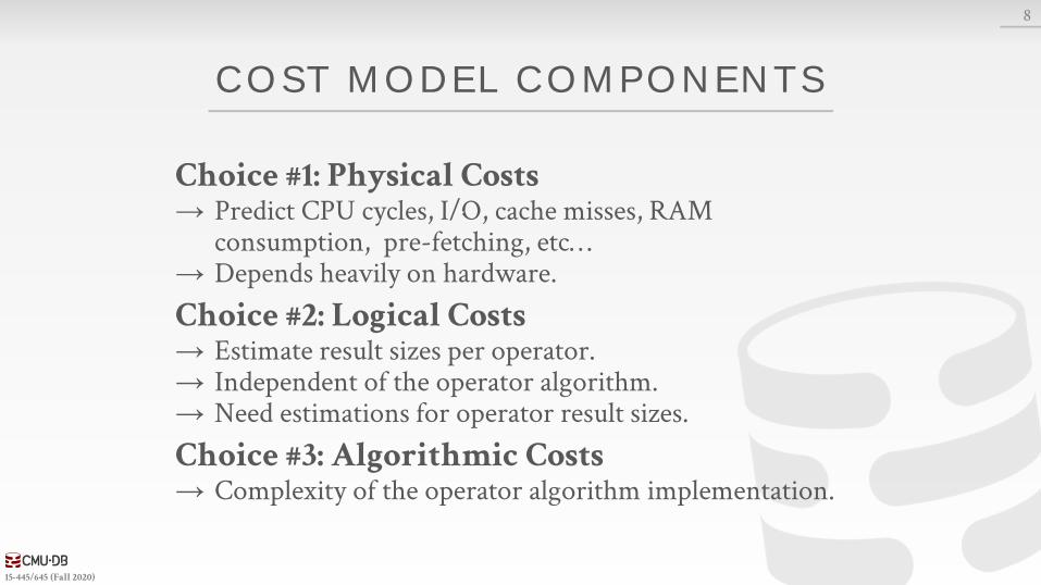
COST MODEL COMPONENTS

Choice #1: Physical Costs→ Predict CPU cycles, I/O, cache misses, RAM

consumption, pre-fetching, etc…→ Depends heavily on hardware.

Choice #2: Logical Costs→ Estimate result sizes per operator.→ Independent of the operator algorithm.→ Need estimations for operator result sizes.

Choice #3: Algorithmic Costs→ Complexity of the operator algorithm implementation.

8

15-445/645 (Fall 2020)

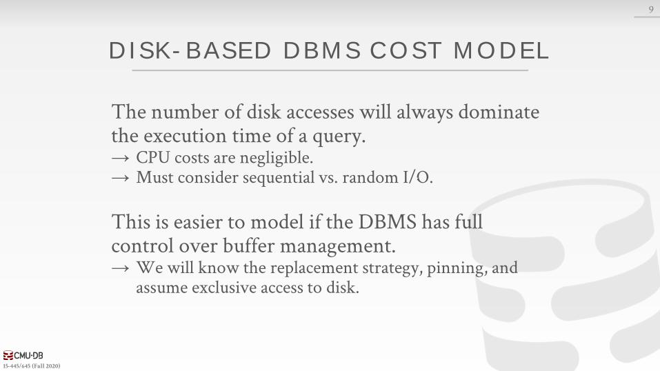
DISK-BASED DBMS COST MODEL

The number of disk accesses will always dominate the execution time of a query.→ CPU costs are negligible.→ Must consider sequential vs. random I/O.

This is easier to model if the DBMS has full control over buffer management.→ We will know the replacement strategy, pinning, and

assume exclusive access to disk.

9

15-445/645 (Fall 2020)

POSTGRES COST MODEL

Uses a combination of CPU and I/O costs that are weighted by “magic” constant factors.

Default settings are obviously for a disk-resident database without a lot of memory:→ Processing a tuple in memory is 400x faster than reading

a tuple from disk.→ Sequential I/O is 4x faster than random I/O.

10

15-445/645 (Fall 2020)

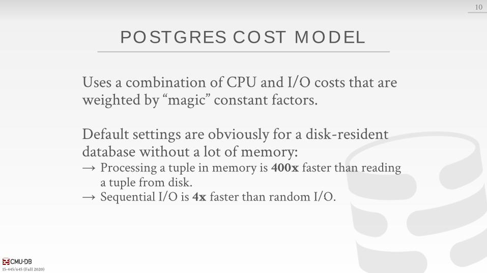
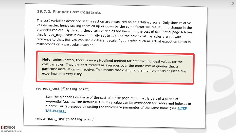
POSTGRES COST MODEL

Uses a combination of CPU and I/O costs that are weighted by “magic” constant factors.

Default settings are obviously for a disk-resident database without a lot of memory:→ Processing a tuple in memory is 400x faster than reading

a tuple from disk.→ Sequential I/O is 4x faster than random I/O.

10

15-445/645 (Fall 2020)

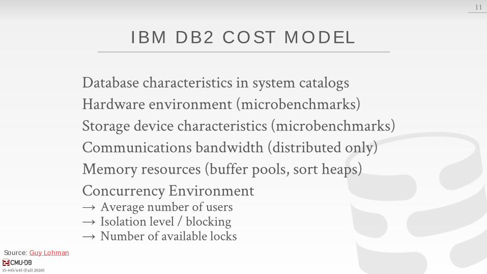
IBM DB2 COST MODEL

Database characteristics in system catalogs

Hardware environment (microbenchmarks)

Storage device characteristics (microbenchmarks)

Communications bandwidth (distributed only)

Memory resources (buffer pools, sort heaps)

Concurrency Environment→ Average number of users→ Isolation level / blocking→ Number of available locks

11

Source: Guy Lohman

15-445/645 (Fall 2020)

STATISTICS

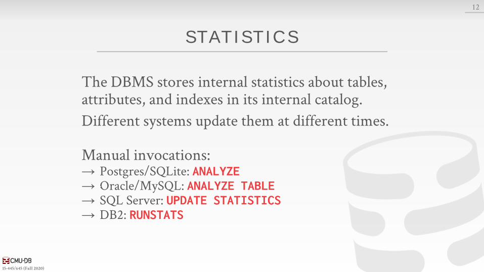
The DBMS stores internal statistics about tables, attributes, and indexes in its internal catalog.

Different systems update them at different times.

Manual invocations:→ Postgres/SQLite: ANALYZE→ Oracle/MySQL: ANALYZE TABLE→ SQL Server: UPDATE STATISTICS→ DB2: RUNSTATS

12

15-445/645 (Fall 2020)

STATISTICS

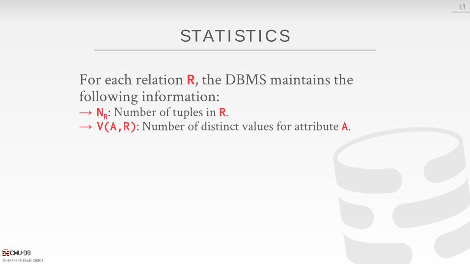
For each relation R, the DBMS maintains the following information:→ NR: Number of tuples in R.→ V(A,R): Number of distinct values for attribute A.

13

15-445/645 (Fall 2020)

DERIVABLE STATISTICS

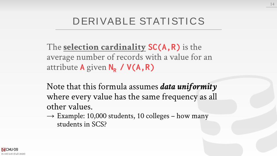
The selection cardinality SC(A,R) is the average number of records with a value for an attribute A given NR / V(A,R)

Note that this formula assumes data uniformitywhere every value has the same frequency as all other values.→ Example: 10,000 students, 10 colleges – how many

students in SCS?

14

15-445/645 (Fall 2020)

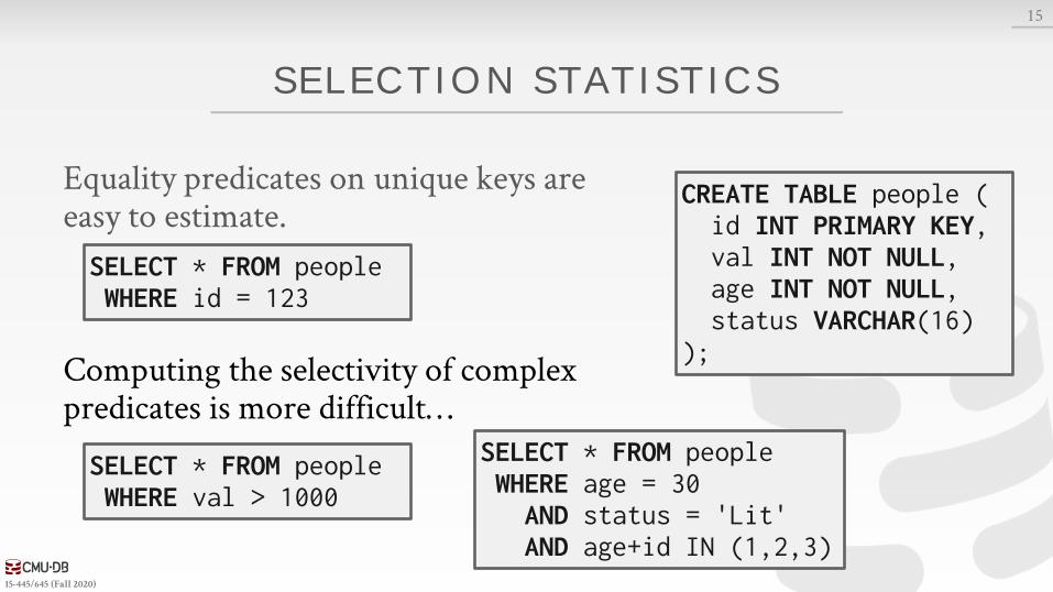
SELECTION STATISTICS

Equality predicates on unique keys are easy to estimate.

Computing the selectivity of complex predicates is more difficult…

15

SELECT * FROM people WHERE id = 123

SELECT * FROM people WHERE val > 1000

SELECT * FROM people WHERE age = 30AND status = 'Lit'AND age+id IN (1,2,3)

CREATE TABLE people (id INT PRIMARY KEY,val INT NOT NULL,age INT NOT NULL,status VARCHAR(16)

);

15-445/645 (Fall 2020)

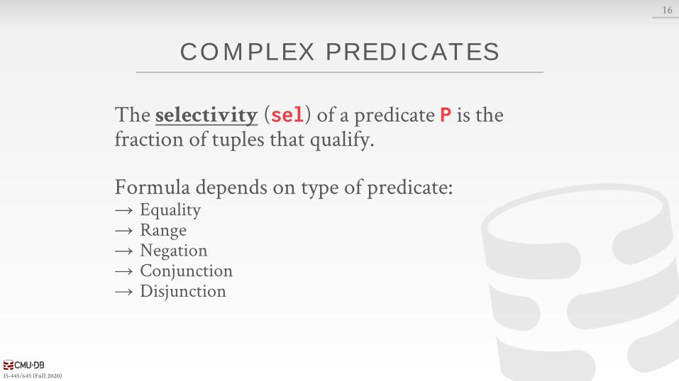
COMPLEX PREDICATES

The selectivity (sel) of a predicate P is the fraction of tuples that qualify.

Formula depends on type of predicate:→ Equality→ Range→ Negation→ Conjunction→ Disjunction

16

15-445/645 (Fall 2020)

COMPLEX PREDICATES

The selectivity (sel) of a predicate P is the fraction of tuples that qualify.

Formula depends on type of predicate:→ Equality→ Range→ Negation→ Conjunction→ Disjunction

16

15-445/645 (Fall 2020)

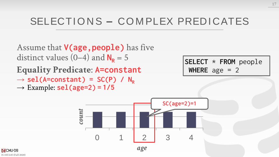
SELECTIONS COMPLEX PREDICATES

Assume that V(age,people) has five distinct values (0–4) and NR = 5

Equality Predicate: A=constant→ sel(A=constant) = SC(P) / NR→ Example: sel(age=2) =

17

0 1 2 3 4

cou

nt

age

SC(age=2)=1

SELECT * FROM people WHERE age = 2

1/5

15-445/645 (Fall 2020)

0 1 2 3 4

cou

nt

age

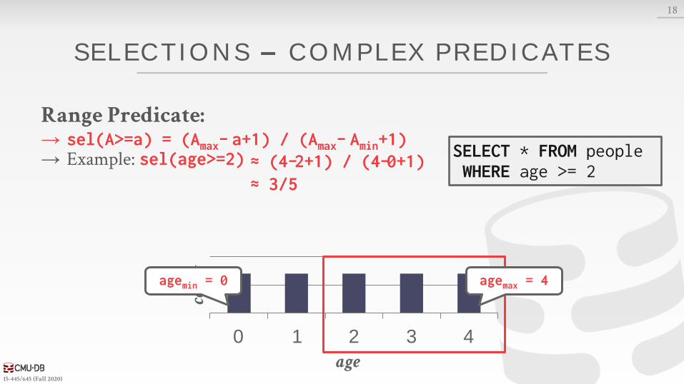
SELECTIONS COMPLEX PREDICATES

Range Predicate:→ sel(A>=a) = (Amax– a+1) / (Amax– Amin+1)→ Example: sel(age>=2)

18

≈ (4–2+1) / (4–0+1)≈ 3/5

agemin = 0

SELECT * FROM people WHERE age >= 2

agemax = 4

15-445/645 (Fall 2020)

0 1 2 3 4

cou

nt

age

SELECTIONS COMPLEX PREDICATES

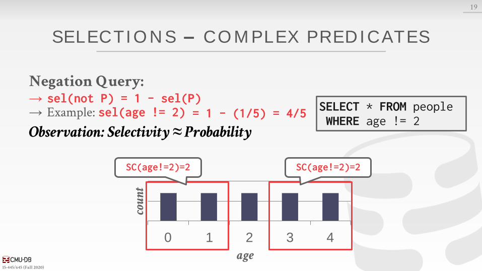
Negation Query:→ sel(not P) = 1 – sel(P)→ Example: sel(age != 2)

Observation: Selectivity ≈ Probability

19

= 1 – (1/5) = 4/5

SC(age!=2)=2 SC(age!=2)=2

SELECT * FROM people WHERE age != 2

15-445/645 (Fall 2020)

SELECTIONS COMPLEX PREDICATES

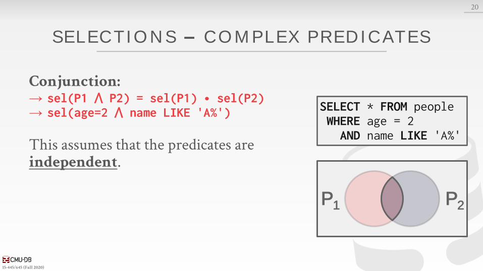
Conjunction: → sel(P1 ⋀ P2) = sel(P1) ∙ sel(P2)→ sel(age=2 ⋀ name LIKE 'A%')

This assumes that the predicates are independent.

20

SELECT * FROM people WHERE age = 2AND name LIKE 'A%'

P1 P2

15-445/645 (Fall 2020)

SELECTIONS COMPLEX PREDICATES

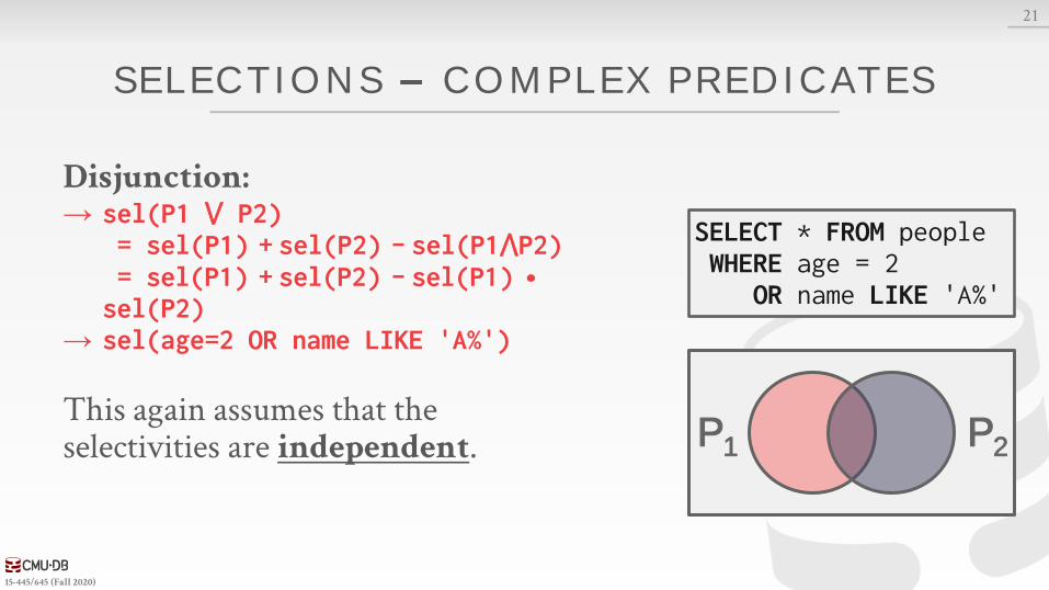
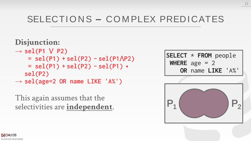
Disjunction: → sel(P1 ⋁ P2)

= sel(P1) + sel(P2) – sel(P1⋀P2)= sel(P1) + sel(P2) – sel(P1) ∙

sel(P2)→ sel(age=2 OR name LIKE 'A%')

This again assumes that theselectivities are independent.

21

SELECT * FROM people WHERE age = 2

OR name LIKE 'A%'

P1 P2

15-445/645 (Fall 2020)

SELECTIONS COMPLEX PREDICATES

Disjunction: → sel(P1 ⋁ P2)

= sel(P1) + sel(P2) – sel(P1⋀P2)= sel(P1) + sel(P2) – sel(P1) ∙

sel(P2)→ sel(age=2 OR name LIKE 'A%')

This again assumes that theselectivities are independent.

21

SELECT * FROM people WHERE age = 2

OR name LIKE 'A%'

P1 P2

15-445/645 (Fall 2020)

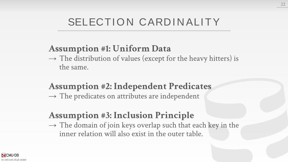
SELECTION CARDINALIT Y

Assumption #1: Uniform Data→ The distribution of values (except for the heavy hitters) is

the same.

Assumption #2: Independent Predicates→ The predicates on attributes are independent

Assumption #3: Inclusion Principle→ The domain of join keys overlap such that each key in the

inner relation will also exist in the outer table.

22

15-445/645 (Fall 2020)

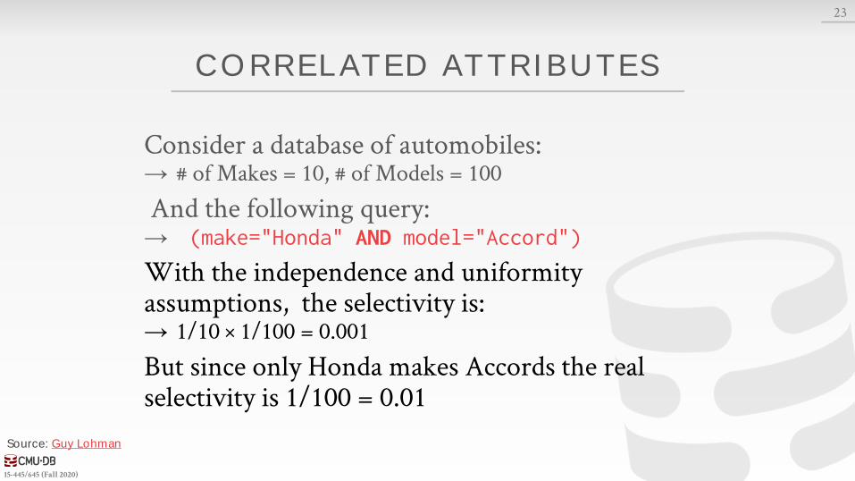
CORREL ATED AT TRIBUTES

Consider a database of automobiles:→ # of Makes = 10, # of Models = 100

And the following query:→ (make="Honda" AND model="Accord")

With the independence and uniformity assumptions, the selectivity is:→ 1/10 × 1/100 = 0.001

But since only Honda makes Accords the real selectivity is 1/100 = 0.01

23

Source: Guy Lohman

15-445/645 (Fall 2020)

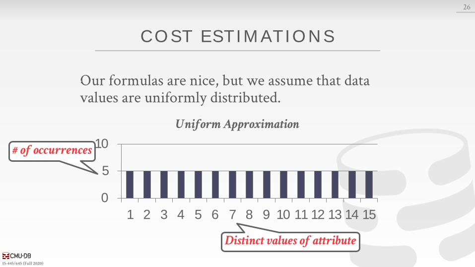
COST ESTIMATIONS

Our formulas are nice, but we assume that data values are uniformly distributed.

26

0

5

10

1 2 3 4 5 6 7 8 9 10 11 12 13 14 15

Uniform Approximation

Distinct values of attribute

# of occurrences

15-445/645 (Fall 2020)

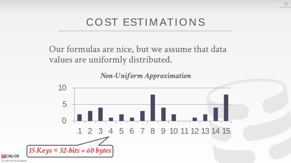
COST ESTIMATIONS

Our formulas are nice, but we assume that data values are uniformly distributed.

27

0

5

10

1 2 3 4 5 6 7 8 9 10 11 12 13 14 15

Non-Uniform Approximation

15 Keys × 32-bits = 60 bytes

15-445/645 (Fall 2020)

0

5

10

1 2 3 4 5 6 7 8 9 10 11 12 13 14 15

Non-Uniform Approximation

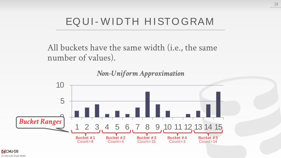
EQUI-WIDTH HISTOGRAM

All buckets have the same width (i.e., the same number of values).

28

Bucket #1Count=8

Bucket #2Count=4

Bucket #3Count=15

Bucket #4Count=3

Bucket #5Count=14

Bucket Ranges

15-445/645 (Fall 2020)

EQUI-WIDTH HISTOGRAM

All buckets have the same width (i.e., the same number of values).

28

Bucket #1Count=8

Bucket #2Count=4

Bucket #3Count=15

Bucket #4Count=3

Bucket #5Count=14

0

5

10

15

1-3 4-6 7-9 10-12 13-15

Equi-Width Histogram

Bucket Ranges

15-445/645 (Fall 2020)

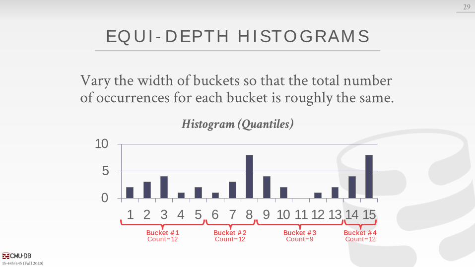
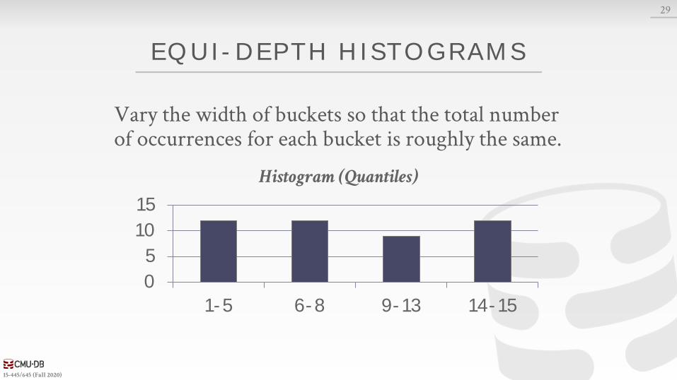
EQUI-DEPTH HISTOGRAMS

Vary the width of buckets so that the total number of occurrences for each bucket is roughly the same.

29

0

5

10

1 2 3 4 5 6 7 8 9 10 11 12 13 14 15

Histogram (Quantiles)

Bucket #1Count=12

Bucket #2Count=12

Bucket #3Count=9

Bucket #4Count=12

15-445/645 (Fall 2020)

EQUI-DEPTH HISTOGRAMS

Vary the width of buckets so that the total number of occurrences for each bucket is roughly the same.

29

0

5

10

15

1-5 6-8 9-13 14-15

Histogram (Quantiles)

15-445/645 (Fall 2020)

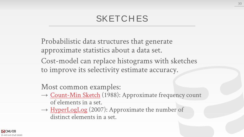
SKETCHES

Probabilistic data structures that generate approximate statistics about a data set.

Cost-model can replace histograms with sketches to improve its selectivity estimate accuracy.

Most common examples:→ Count-Min Sketch (1988): Approximate frequency count

of elements in a set.→ HyperLogLog (2007): Approximate the number of

distinct elements in a set.

30

15-445/645 (Fall 2020)

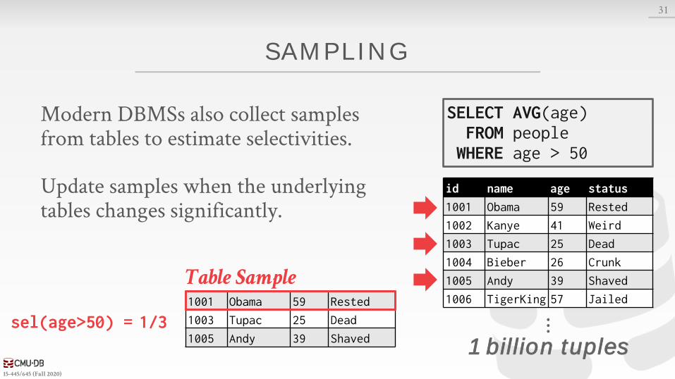
SAMPLING

Modern DBMSs also collect samples from tables to estimate selectivities.

Update samples when the underlying tables changes significantly.

31

⋮1 billion tuples

1/3sel(age>50) =

SELECT AVG(age)FROM people WHERE age > 50

id name age status

1001 Obama 59 Rested

1002 Kanye 41 Weird

1003 Tupac 25 Dead

1004 Bieber 26 Crunk

1005 Andy 39 Shaved

1006 TigerKing 57 Jailed1001 Obama 59 Rested

1003 Tupac 25 Dead

1005 Andy 39 Shaved

Table Sample

15-445/645 (Fall 2020)

OBSERVATION

Now that we can (roughly) estimate the selectivity of predicates, what can we do with them?

32

15-445/645 (Fall 2020)

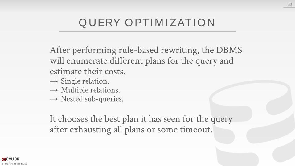
QUERY OPTIMIZATION

After performing rule-based rewriting, the DBMS will enumerate different plans for the query and estimate their costs.→ Single relation.→ Multiple relations.→ Nested sub-queries.

It chooses the best plan it has seen for the query after exhausting all plans or some timeout.

33

15-445/645 (Fall 2020)

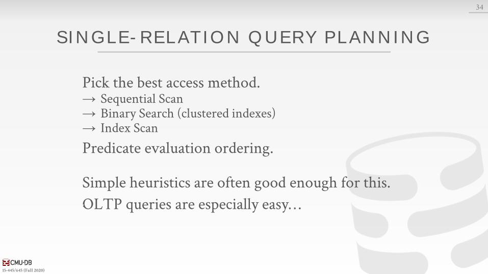
SINGLE-REL ATION QUERY PL ANNING

Pick the best access method.→ Sequential Scan→ Binary Search (clustered indexes)→ Index Scan

Predicate evaluation ordering.

Simple heuristics are often good enough for this.

OLTP queries are especially easy…

34

15-445/645 (Fall 2020)

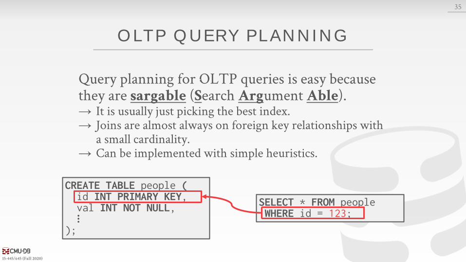
OLTP QUERY PL ANNING

Query planning for OLTP queries is easy because they are sargable (Search Argument Able).→ It is usually just picking the best index.→ Joins are almost always on foreign key relationships with

a small cardinality.→ Can be implemented with simple heuristics.

35

CREATE TABLE people (id INT PRIMARY KEY,val INT NOT NULL,⋮

);

SELECT * FROM peopleWHERE id = 123;

15-445/645 (Fall 2020)

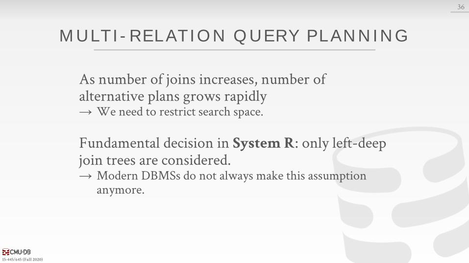
MULTI-REL ATION QUERY PL ANNING

As number of joins increases, number of alternative plans grows rapidly→ We need to restrict search space.

Fundamental decision in System R: only left-deep join trees are considered.→ Modern DBMSs do not always make this assumption

anymore.

36

15-445/645 (Fall 2020)

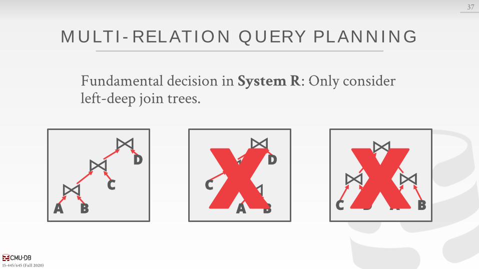
MULTI-REL ATION QUERY PL ANNING

Fundamental decision in System R: Only consider left-deep join trees.

37

⨝

⨝⨝

A B

C

D

⨝

⨝⨝

A B

C

D

⨝⨝

⨝

A BC D

15-445/645 (Fall 2020)

MULTI-REL ATION QUERY PL ANNING

Fundamental decision in System R: Only consider left-deep join trees.

37

⨝

⨝⨝

A B

C

D

⨝

⨝⨝

A B

C

D

⨝⨝

⨝

A BC DX X

15-445/645 (Fall 2020)

MULTI-REL ATION QUERY PL ANNING

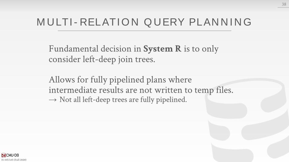
Fundamental decision in System R is to only consider left-deep join trees.

Allows for fully pipelined plans where intermediate results are not written to temp files.→ Not all left-deep trees are fully pipelined.

38

15-445/645 (Fall 2020)

MULTI-REL ATION QUERY PL ANNING

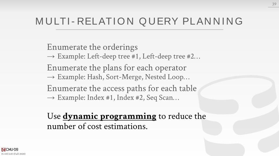
Enumerate the orderings→ Example: Left-deep tree #1, Left-deep tree #2…

Enumerate the plans for each operator→ Example: Hash, Sort-Merge, Nested Loop…

Enumerate the access paths for each table→ Example: Index #1, Index #2, Seq Scan…

Use dynamic programming to reduce the number of cost estimations.

39

15-445/645 (Fall 2020)

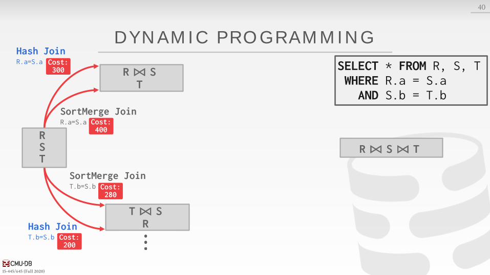
DYNAMIC PROGRAMMING

40

SortMerge JoinR.a=S.a

SortMerge JoinT.b=S.b

Hash JoinT.b=S.b

R ⨝ ST

T ⨝ SR

R ⨝ S ⨝ T

Hash JoinR.a=S.a SELECT * FROM R, S, T

WHERE R.a = S.aAND S.b = T.b

Cost: 300

Cost: 400

Cost: 280

Cost: 200

RST

15-445/645 (Fall 2020)

DYNAMIC PROGRAMMING

40

Hash JoinT.b=S.b

R ⨝ ST

T ⨝ SR

R ⨝ S ⨝ T

Hash JoinR.a=S.a

Hash JoinS.b=T.b

SortMerge JoinS.b=T.b

SortMerge JoinS.a=R.a

Hash JoinS.a=R.a

SELECT * FROM R, S, TWHERE R.a = S.aAND S.b = T.b

Cost: 300

Cost: 200

Cost: 450

Cost: 300

Cost: 400

Cost: 380

RST

15-445/645 (Fall 2020)

DYNAMIC PROGRAMMING

40

Hash JoinT.b=S.b

R ⨝ ST

T ⨝ SR

R ⨝ S ⨝ T

Hash JoinR.a=S.a

Hash JoinS.b=T.b

SortMerge JoinS.a=R.a

SELECT * FROM R, S, TWHERE R.a = S.aAND S.b = T.b

Cost: 300

Cost: 200

Cost: 300

Cost: 380

RST

15-445/645 (Fall 2020)

DYNAMIC PROGRAMMING

40

Hash JoinT.b=S.b

R ⨝ ST

T ⨝ SR

R ⨝ S ⨝ TSortMerge JoinS.a=R.a

SELECT * FROM R, S, TWHERE R.a = S.aAND S.b = T.b

Cost: 200

Cost: 300

RST

15-445/645 (Fall 2020)

CANDIDATE PL AN EXAMPLE

How to generate plans for search algorithm:→ Enumerate relation orderings→ Enumerate join algorithm choices→ Enumerate access method choices

No real DBMSs does it this way.It’s actually more messy…

41

SELECT * FROM R, S, TWHERE R.a = S.aAND S.b = T.b

15-445/645 (Fall 2020)

CANDIDATE PL ANS

Step #1: Enumerate relation orderings

42

⨝

⨝

T R

S ⨝

⨝

S T

R ×

⨝

R S

T

⨝

⨝

R S

T ⨝

⨝

S R

T ×

⨝

S T

R

Prune plans with cross-products immediately!

15-445/645 (Fall 2020)

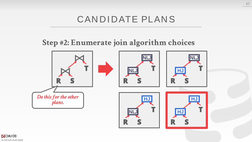
CANDIDATE PL ANS

Step #2: Enumerate join algorithm choices

43

⨝

⨝

R S

T

Do this for the other plans.

R S

TNLJ

NLJ

R S

THJ

NLJ

R S

TNLJ

HJ

R S

T

HJ

HJ

15-445/645 (Fall 2020)

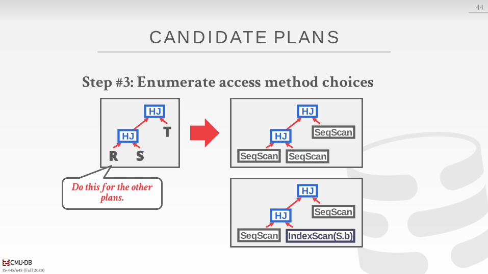
CANDIDATE PL ANS

Step #3: Enumerate access method choices

44

R S

T

HJ

HJ

Do this for the other plans.

HJ

HJ

SeqScan SeqScan

SeqScan

HJ

HJ

SeqScan IndexScan(S.b)

SeqScan

15-445/645 (Fall 2020)

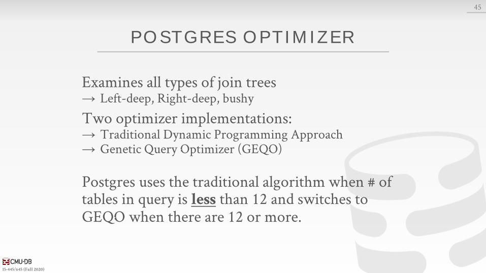
POSTGRES OPTIMIZER

Examines all types of join trees→ Left-deep, Right-deep, bushy

Two optimizer implementations:→ Traditional Dynamic Programming Approach→ Genetic Query Optimizer (GEQO)

Postgres uses the traditional algorithm when # of tables in query is less than 12 and switches to GEQO when there are 12 or more.

45

15-445/645 (Fall 2020)

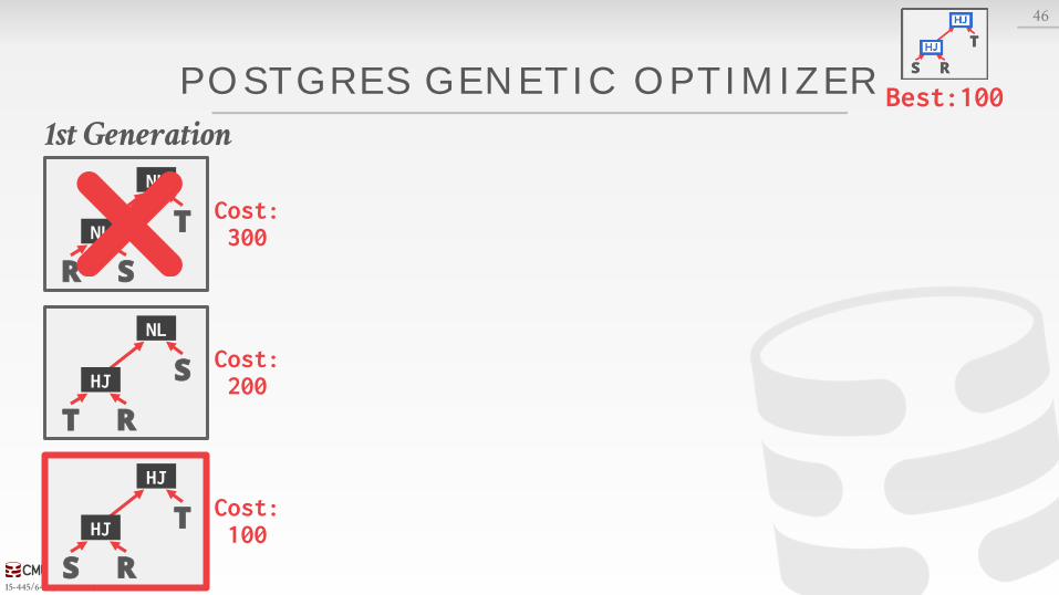
POSTGRES GENETIC OPTIMIZER

46

Best:1001st Generation

R S

T

NL

NLCost:300

T R

S

NL

HJ

S R

T

HJ

HJ

Cost:200

Cost:100

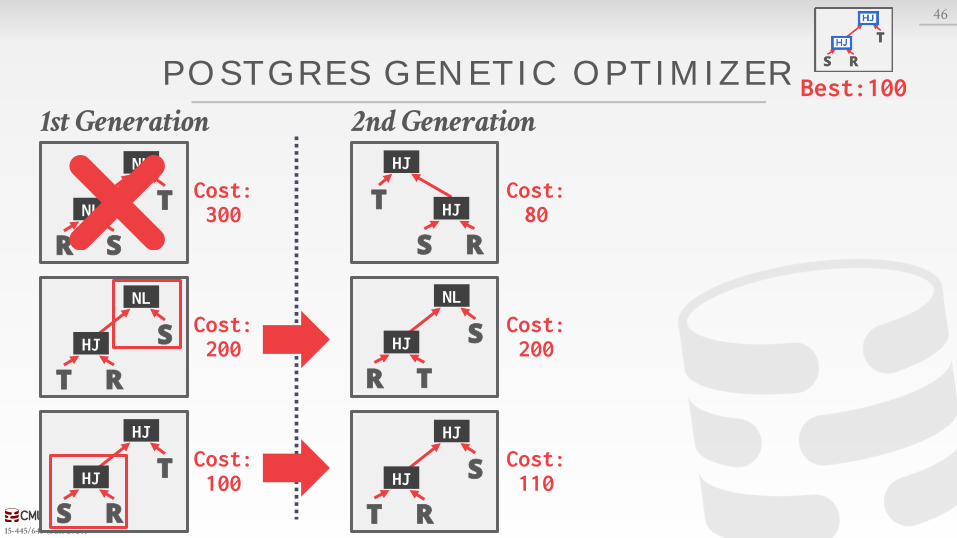
15-445/645 (Fall 2020)

POSTGRES GENETIC OPTIMIZER

46

Best:1001st Generation 2nd Generation

R S

T

NL

NLCost:300

T R

S

NL

HJ

S R

T

HJ

HJ

Cost:200

Cost:100

S R

T

HJ

HJ

R T

S

NL

HJ

T R

S

HJ

HJ

Cost:80

Cost:200

Cost:110

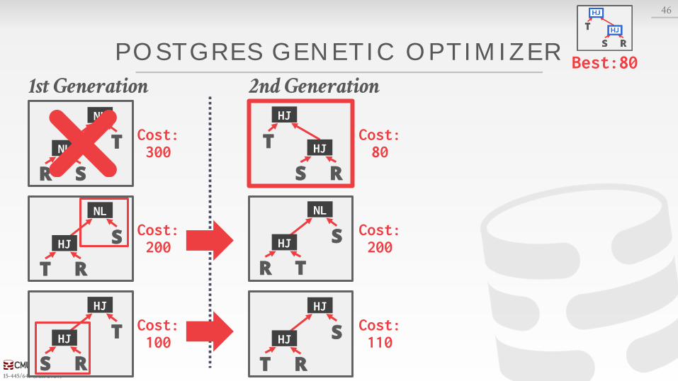
15-445/645 (Fall 2020)

POSTGRES GENETIC OPTIMIZER

46

1st Generation 2nd GenerationBest:80

R S

T

NL

NLCost:300

T R

S

NL

HJ

S R

T

HJ

HJ

Cost:200

Cost:100

S R

T

HJ

HJ

R T

S

NL

HJ

T R

S

HJ

HJ

Cost:80

Cost:200

Cost:110

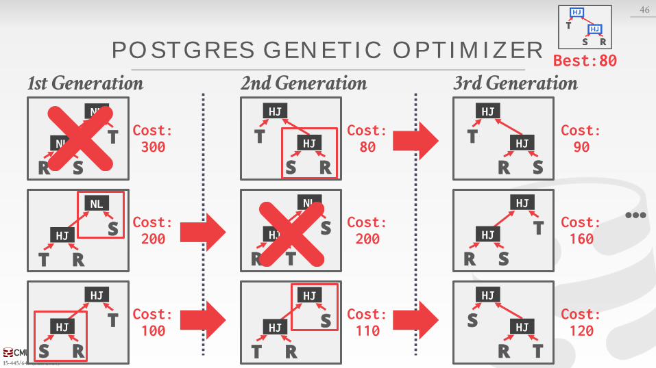
15-445/645 (Fall 2020)

POSTGRES GENETIC OPTIMIZER

46

1st Generation 2nd Generation 3rd Generation

…

Best:80

R S

T

NL

NLCost:300

T R

S

NL

HJ

S R

T

HJ

HJ

Cost:200

Cost:100

S R

T

HJ

HJ

R T

S

NL

HJ

T R

S

HJ

HJ

Cost:80

Cost:200

Cost:110

R S

T

HJ

HJ

R S

T

HJ

HJ

R T

S

HJ

HJ

Cost:90

Cost:160

Cost:120

15-445/645 (Fall 2020)

CONCLUSION

Filter early as possible.

Selectivity estimations→ Uniformity→ Independence→ Histograms→ Join selectivity

Dynamic programming for join orderings

Again, query optimization is hard…

47

15-445/645 (Fall 2020)

NEXT CL ASS

Transactions!→ aka the second hardest part about database systems

48