Embed Size (px)
Citation preview
150C Causal Inference
Randomized Experiments 2
Jonathan Mummolo
1 / 104
Outline
1 Hypothesis Testing in Small Samples
2 Using Covariates in Experiments
3 Examples
Social Pressure Experiment
Tax Compliance
Labor Market Discrimination
Job Training Partnership Act (JTPA)
4 Threats to Validity and Ethics
2 / 104
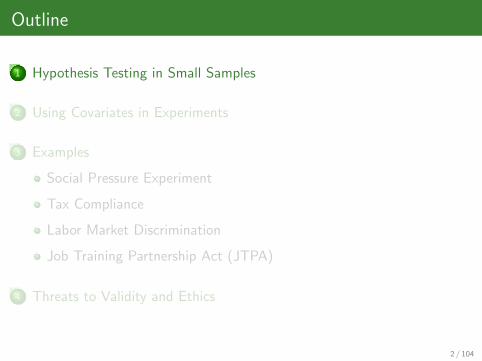
Regression to Estimate the Average Treatment Effect
R Code> library(sandwich)
> library(lmtest)
>
> lout <- lm(earnings~assignmt,data=d)
> coeftest(lout,vcov = vcovHC(lout, type = "HC1")) # matches Stata
t test of coefficients:
Estimate Std. Error t value Pr(>|t|)
(Intercept) 15040.50 265.38 56.6752 < 2.2e-16 ***
assignmt 1159.43 330.46 3.5085 0.0004524 ***
---
3 / 104
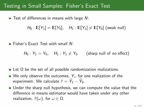
Testing in Small Samples: Fisher’s Exact Test
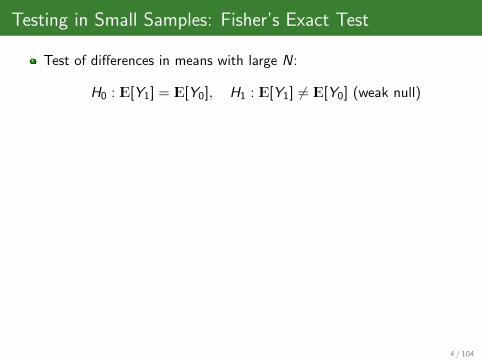
Test of differences in means with large N:
H0 : IE[Y1] = IE[Y0], H1 : IE[Y1] 6= IE[Y0] (weak null)
Fisher’s Exact Test with small N:
H0 : Y1 = Y0, H1 : Y1 6= Y0 (sharp null of no effect)
Let Ω be the set of all possible randomization realizations.
We only observe the outcomes, Yi , for one realization of theexperiment. We calculate τ = Y1 − Y0.
Under the sharp null hypothesis, we can compute the value that thedifference in means estimator would have taken under any otherrealization, τ(ω), for ω ∈ Ω.
4 / 104
Testing in Small Samples: Fisher’s Exact Test
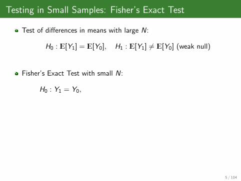
Test of differences in means with large N:
H0 : IE[Y1] = IE[Y0], H1 : IE[Y1] 6= IE[Y0] (weak null)
Fisher’s Exact Test with small N:
H0 : Y1 = Y0,
H1 : Y1 6= Y0 (sharp null of no effect)
Let Ω be the set of all possible randomization realizations.
We only observe the outcomes, Yi , for one realization of theexperiment. We calculate τ = Y1 − Y0.
Under the sharp null hypothesis, we can compute the value that thedifference in means estimator would have taken under any otherrealization, τ(ω), for ω ∈ Ω.
5 / 104
Testing in Small Samples: Fisher’s Exact Test
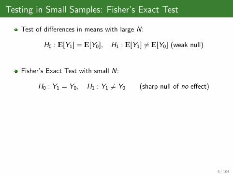
Test of differences in means with large N:
H0 : IE[Y1] = IE[Y0], H1 : IE[Y1] 6= IE[Y0] (weak null)
Fisher’s Exact Test with small N:
H0 : Y1 = Y0, H1 : Y1 6= Y0 (sharp null of no effect)
Let Ω be the set of all possible randomization realizations.
We only observe the outcomes, Yi , for one realization of theexperiment. We calculate τ = Y1 − Y0.
Under the sharp null hypothesis, we can compute the value that thedifference in means estimator would have taken under any otherrealization, τ(ω), for ω ∈ Ω.
6 / 104
Testing in Small Samples: Fisher’s Exact Test
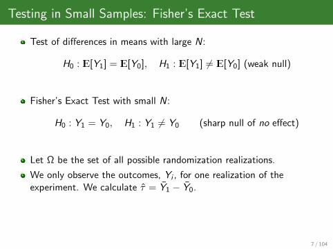
Test of differences in means with large N:
H0 : IE[Y1] = IE[Y0], H1 : IE[Y1] 6= IE[Y0] (weak null)
Fisher’s Exact Test with small N:
H0 : Y1 = Y0, H1 : Y1 6= Y0 (sharp null of no effect)
Let Ω be the set of all possible randomization realizations.
We only observe the outcomes, Yi , for one realization of theexperiment. We calculate τ = Y1 − Y0.
Under the sharp null hypothesis, we can compute the value that thedifference in means estimator would have taken under any otherrealization, τ(ω), for ω ∈ Ω.
7 / 104
Testing in Small Samples: Fisher’s Exact Test
Test of differences in means with large N:
H0 : IE[Y1] = IE[Y0], H1 : IE[Y1] 6= IE[Y0] (weak null)
Fisher’s Exact Test with small N:
H0 : Y1 = Y0, H1 : Y1 6= Y0 (sharp null of no effect)
Let Ω be the set of all possible randomization realizations.
We only observe the outcomes, Yi , for one realization of theexperiment. We calculate τ = Y1 − Y0.
Under the sharp null hypothesis, we can compute the value that thedifference in means estimator would have taken under any otherrealization, τ(ω), for ω ∈ Ω.
8 / 104
Testing in Small Samples: Fisher’s Exact Test
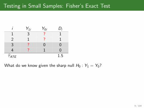
i Y1i Y0i Di
1 3 ? 12 1 ? 13 ? 0 04 ? 1 0
τATE 1.5
What do we know given the sharp null H0 : Y1 = Y0?
9 / 104
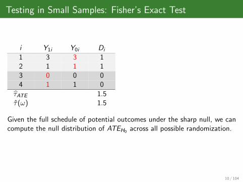
Testing in Small Samples: Fisher’s Exact Test
i Y1i Y0i Di
1 3 3 12 1 1 13 0 0 04 1 1 0
τATE 1.5τ(ω) 1.5
Given the full schedule of potential outcomes under the sharp null, we cancompute the null distribution of ATEH0 across all possible randomization.
10 / 104
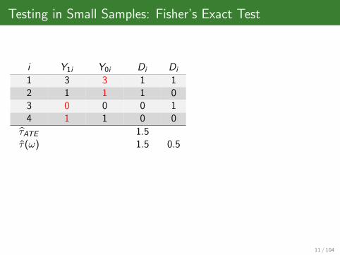
Testing in Small Samples: Fisher’s Exact Test
i Y1i Y0i Di Di
1 3 3 1 12 1 1 1 03 0 0 0 14 1 1 0 0
τATE 1.5τ(ω) 1.5 0.5
11 / 104
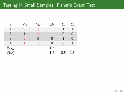
Testing in Small Samples: Fisher’s Exact Test
i Y1i Y0i Di Di Di
1 3 3 1 1 12 1 1 1 0 03 0 0 0 1 04 1 1 0 0 1
τATE 1.5τ(ω) 1.5 0.5 1.5
12 / 104
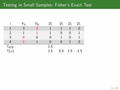
Testing in Small Samples: Fisher’s Exact Test
i Y1i Y0i Di Di Di Di
1 3 3 1 1 1 02 1 1 1 0 0 13 0 0 0 1 0 14 1 1 0 0 1 0
τATE 1.5τ(ω) 1.5 0.5 1.5 -1.5
13 / 104
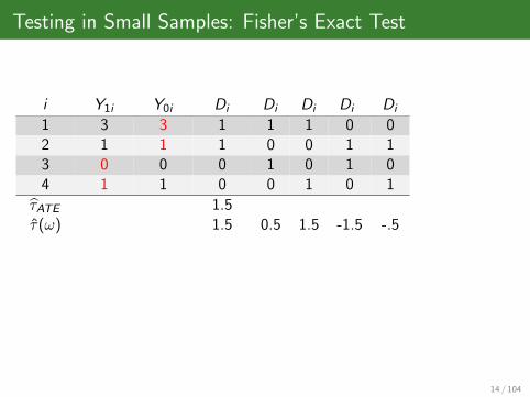
Testing in Small Samples: Fisher’s Exact Test
i Y1i Y0i Di Di Di Di Di
1 3 3 1 1 1 0 02 1 1 1 0 0 1 13 0 0 0 1 0 1 04 1 1 0 0 1 0 1
τATE 1.5τ(ω) 1.5 0.5 1.5 -1.5 -.5
14 / 104
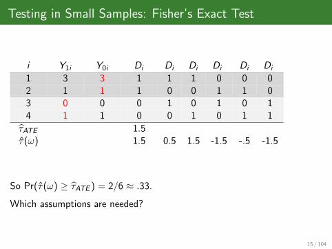
Testing in Small Samples: Fisher’s Exact Test
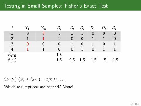
i Y1i Y0i Di Di Di Di Di Di
1 3 3 1 1 1 0 0 02 1 1 1 0 0 1 1 03 0 0 0 1 0 1 0 14 1 1 0 0 1 0 1 1
τATE 1.5τ(ω) 1.5 0.5 1.5 -1.5 -.5 -1.5
So Pr(τ(ω) ≥ τATE ) = 2/6 ≈ .33.
Which assumptions are needed?
15 / 104
Testing in Small Samples: Fisher’s Exact Test
i Y1i Y0i Di Di Di Di Di Di
1 3 3 1 1 1 0 0 02 1 1 1 0 0 1 1 03 0 0 0 1 0 1 0 14 1 1 0 0 1 0 1 1
τATE 1.5τ(ω) 1.5 0.5 1.5 -1.5 -.5 -1.5
So Pr(τ(ω) ≥ τATE ) = 2/6 ≈ .33.
Which assumptions are needed? None!
16 / 104
Outline
1 Hypothesis Testing in Small Samples
2 Using Covariates in Experiments
3 Examples
Social Pressure Experiment
Tax Compliance
Labor Market Discrimination
Job Training Partnership Act (JTPA)
4 Threats to Validity and Ethics
17 / 104
Covariates and Experiments
Y1 Y0
Y1 Y0
Y1 Y0
Y1 Y0
Y1 Y0
Y1 Y0
Y1 Y0 Y1 Y0 Y1 Y0Y1 Y0 Y1 Y0 Y1 Y0 Y1 Y0 Y1 Y0 Y1 Y0
X
X
X
X
XX
X X X X X X
18 / 104
Controlling for All Confounders, Seen and Unseen
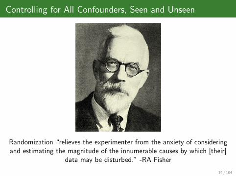
Randomization “relieves the experimenter from the anxiety of consideringand estimating the magnitude of the innumerable causes by which [their]
data may be disturbed.” -RA Fisher
19 / 104
Covariates for Balance Checks
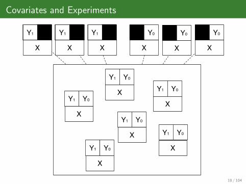
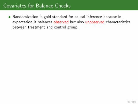
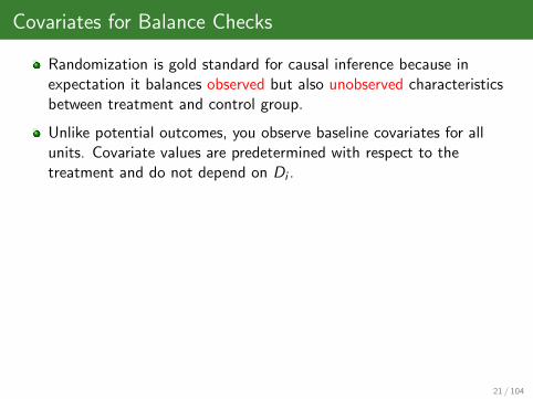
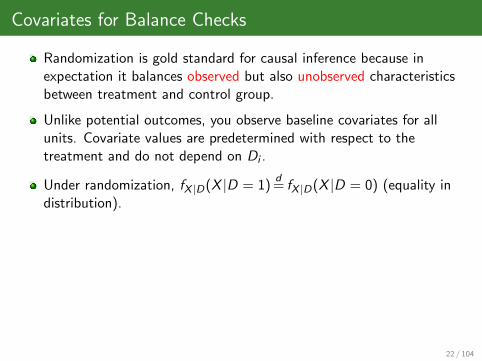
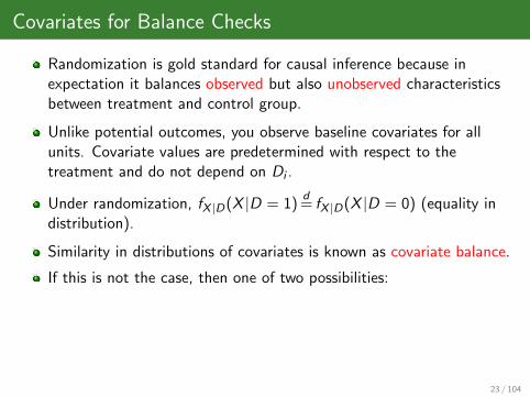
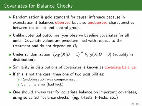
Randomization is gold standard for causal inference because inexpectation it balances observed but also unobserved characteristicsbetween treatment and control group.
Unlike potential outcomes, you observe baseline covariates for allunits. Covariate values are predetermined with respect to thetreatment and do not depend on Di .
Under randomization, fX |D(X |D = 1)d= fX |D(X |D = 0) (equality in
distribution).
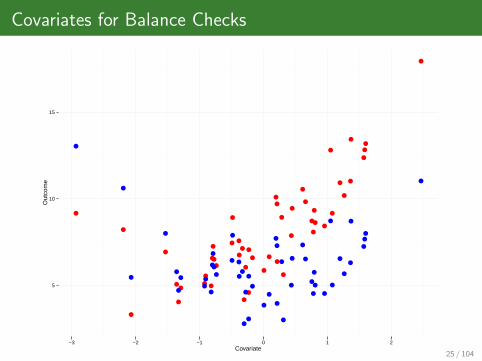
Similarity in distributions of covariates is known as covariate balance.
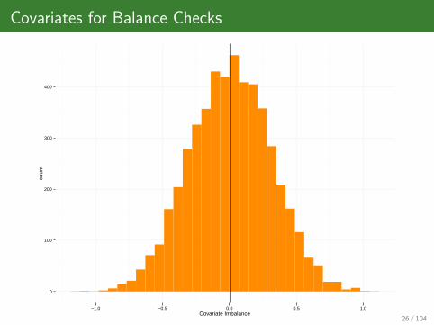
If this is not the case, then one of two possibilities:Randomization was compromised.
Sampling error (bad luck)
One should always test for covariate balance on important covariates,using so called “balance checks” (eg. t-tests, F-tests, etc.)
20 / 104
Covariates for Balance Checks
Randomization is gold standard for causal inference because inexpectation it balances observed but also unobserved characteristicsbetween treatment and control group.
Unlike potential outcomes, you observe baseline covariates for allunits. Covariate values are predetermined with respect to thetreatment and do not depend on Di .
Under randomization, fX |D(X |D = 1)d= fX |D(X |D = 0) (equality in
distribution).
Similarity in distributions of covariates is known as covariate balance.
If this is not the case, then one of two possibilities:Randomization was compromised.
Sampling error (bad luck)
One should always test for covariate balance on important covariates,using so called “balance checks” (eg. t-tests, F-tests, etc.)
21 / 104
Covariates for Balance Checks
Randomization is gold standard for causal inference because inexpectation it balances observed but also unobserved characteristicsbetween treatment and control group.
Unlike potential outcomes, you observe baseline covariates for allunits. Covariate values are predetermined with respect to thetreatment and do not depend on Di .
Under randomization, fX |D(X |D = 1)d= fX |D(X |D = 0) (equality in
distribution).
Similarity in distributions of covariates is known as covariate balance.
If this is not the case, then one of two possibilities:Randomization was compromised.
Sampling error (bad luck)
One should always test for covariate balance on important covariates,using so called “balance checks” (eg. t-tests, F-tests, etc.)
22 / 104
Covariates for Balance Checks
Randomization is gold standard for causal inference because inexpectation it balances observed but also unobserved characteristicsbetween treatment and control group.
Unlike potential outcomes, you observe baseline covariates for allunits. Covariate values are predetermined with respect to thetreatment and do not depend on Di .
Under randomization, fX |D(X |D = 1)d= fX |D(X |D = 0) (equality in
distribution).
Similarity in distributions of covariates is known as covariate balance.
If this is not the case, then one of two possibilities:
Randomization was compromised.
Sampling error (bad luck)
One should always test for covariate balance on important covariates,using so called “balance checks” (eg. t-tests, F-tests, etc.)
23 / 104
Covariates for Balance Checks
Randomization is gold standard for causal inference because inexpectation it balances observed but also unobserved characteristicsbetween treatment and control group.
Unlike potential outcomes, you observe baseline covariates for allunits. Covariate values are predetermined with respect to thetreatment and do not depend on Di .
Under randomization, fX |D(X |D = 1)d= fX |D(X |D = 0) (equality in
distribution).
Similarity in distributions of covariates is known as covariate balance.
If this is not the case, then one of two possibilities:Randomization was compromised.
Sampling error (bad luck)
One should always test for covariate balance on important covariates,using so called “balance checks” (eg. t-tests, F-tests, etc.)
24 / 104
Covariates for Balance Checks
5
10
15
−3 −2 −1 0 1 2Covariate
Out
com
e
25 / 104
Covariates for Balance Checks
0
100
200
300
400
−1.0 −0.5 0.0 0.5 1.0Covariate Imbalance
coun
t
26 / 104
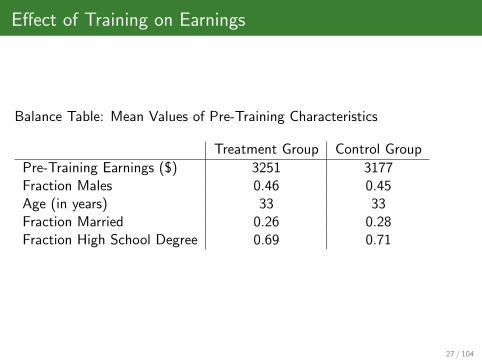
Effect of Training on Earnings
Balance Table: Mean Values of Pre-Training Characteristics
Treatment Group Control Group
Pre-Training Earnings ($) 3251 3177Fraction Males 0.46 0.45Age (in years) 33 33Fraction Married 0.26 0.28Fraction High School Degree 0.69 0.71
27 / 104
Regression Adjusted Estimator for ATE
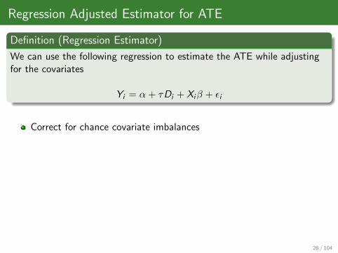
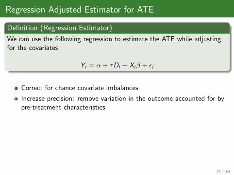
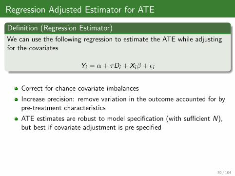
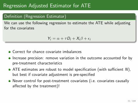
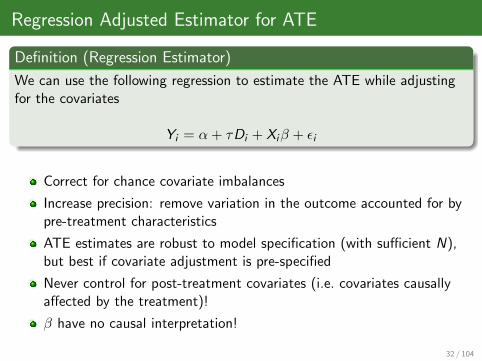
Definition (Regression Estimator)
We can use the following regression to estimate the ATE while adjustingfor the covariates
Yi = α + τDi + Xiβ + εi
Correct for chance covariate imbalances
Increase precision: remove variation in the outcome accounted for bypre-treatment characteristics
ATE estimates are robust to model specification (with sufficient N),but best if covariate adjustment is pre-specified
Never control for post-treatment covariates (i.e. covariates causallyaffected by the treatment)!
β have no causal interpretation!
28 / 104
Regression Adjusted Estimator for ATE
Definition (Regression Estimator)
We can use the following regression to estimate the ATE while adjustingfor the covariates
Yi = α + τDi + Xiβ + εi
Correct for chance covariate imbalances
Increase precision: remove variation in the outcome accounted for bypre-treatment characteristics
ATE estimates are robust to model specification (with sufficient N),but best if covariate adjustment is pre-specified
Never control for post-treatment covariates (i.e. covariates causallyaffected by the treatment)!
β have no causal interpretation!
29 / 104
Regression Adjusted Estimator for ATE
Definition (Regression Estimator)
We can use the following regression to estimate the ATE while adjustingfor the covariates
Yi = α + τDi + Xiβ + εi
Correct for chance covariate imbalances
Increase precision: remove variation in the outcome accounted for bypre-treatment characteristics
ATE estimates are robust to model specification (with sufficient N),but best if covariate adjustment is pre-specified
Never control for post-treatment covariates (i.e. covariates causallyaffected by the treatment)!
β have no causal interpretation!
30 / 104
Regression Adjusted Estimator for ATE
Definition (Regression Estimator)
We can use the following regression to estimate the ATE while adjustingfor the covariates
Yi = α + τDi + Xiβ + εi
Correct for chance covariate imbalances
Increase precision: remove variation in the outcome accounted for bypre-treatment characteristics
ATE estimates are robust to model specification (with sufficient N),but best if covariate adjustment is pre-specified
Never control for post-treatment covariates (i.e. covariates causallyaffected by the treatment)!
β have no causal interpretation!
31 / 104
Regression Adjusted Estimator for ATE
Definition (Regression Estimator)
We can use the following regression to estimate the ATE while adjustingfor the covariates
Yi = α + τDi + Xiβ + εi
Correct for chance covariate imbalances
Increase precision: remove variation in the outcome accounted for bypre-treatment characteristics
ATE estimates are robust to model specification (with sufficient N),but best if covariate adjustment is pre-specified
Never control for post-treatment covariates (i.e. covariates causallyaffected by the treatment)!
β have no causal interpretation!
32 / 104
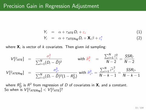
Precision Gain in Regression Adjustment
Yi = α + τATEDi + εi (1)
Yi = α + τATERegDi + Xiβ + ε∗i (2)
where Xi is vector of k covariates. Then given iid sampling:
V [τATE ] =σ2ε∑N
i=1(Di − D)2with σ2
ε =
∑Ni=1 ε
2i
N − 2=
SSRε
N − 2
V [τATEReg ] =σ2ε∗∑N
i=1(Di − D)2(1− R2D)
with σ2ε∗ =
∑Ni=1 ε
∗2i
N − k − 1=
SSRε∗
N − k − 1
where R2D is R2 from regression of D of covariates in Xi and a constant.
So when is V [τATEReg ] < V [τATE ]?
33 / 104
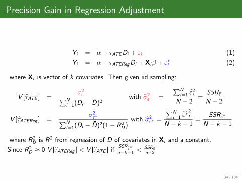
Precision Gain in Regression Adjustment
Yi = α + τATEDi + εi (1)
Yi = α + τATERegDi + Xiβ + ε∗i (2)
where Xi is vector of k covariates. Then given iid sampling:
V [τATE ] =σ2ε∑N
i=1(Di − D)2with σ2
ε =
∑Ni=1 ε
2i
N − 2=
SSRε
N − 2
V [τATEReg ] =σ2ε∗∑N
i=1(Di − D)2(1− R2D)
with σ2ε∗ =
∑Ni=1 ε
∗2i
N − k − 1=
SSRε∗
N − k − 1
where R2D is R2 from regression of D of covariates in Xi and a constant.
Since R2D ≈ 0 V [τATEReg ] < V [τATE ] if
SSRε∗
n−k−1 <SSRε
n−2
34 / 104
Regression Adjusted Estimator for ATE
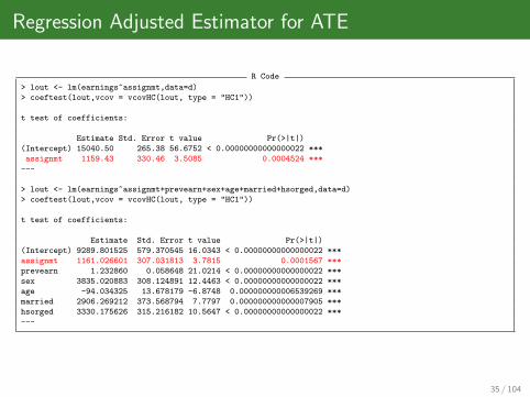
R Code
> lout <- lm(earnings~assignmt,data=d)
> coeftest(lout,vcov = vcovHC(lout, type = "HC1"))
t test of coefficients:
Estimate Std. Error t value Pr(>|t|)
(Intercept) 15040.50 265.38 56.6752 < 0.00000000000000022 ***
assignmt 1159.43 330.46 3.5085 0.0004524 ***
---
> lout <- lm(earnings~assignmt+prevearn+sex+age+married+hsorged,data=d)
> coeftest(lout,vcov = vcovHC(lout, type = "HC1"))
t test of coefficients:
Estimate Std. Error t value Pr(>|t|)
(Intercept) 9289.801525 579.370545 16.0343 < 0.00000000000000022 ***
assignmt 1161.026601 307.031813 3.7815 0.0001567 ***
prevearn 1.232860 0.058648 21.0214 < 0.00000000000000022 ***
sex 3835.020883 308.124891 12.4463 < 0.00000000000000022 ***
age -94.034325 13.678179 -6.8748 0.000000000006539269 ***
married 2906.269212 373.568794 7.7797 0.000000000000007905 ***
hsorged 3330.175626 315.216182 10.5647 < 0.00000000000000022 ***
---
35 / 104
Outline
1 Hypothesis Testing in Small Samples
2 Using Covariates in Experiments
3 Examples
Social Pressure Experiment
Tax Compliance
Labor Market Discrimination
Job Training Partnership Act (JTPA)
4 Threats to Validity and Ethics
36 / 104

Experiments in Popular Culture
37 / 104
The Rise of Experiments
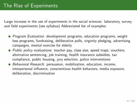
Large increase in the use of experiments in the social sciences: laboratory, survey,and field experiments (see syllabus)
Abbreviated list of examples:
Program Evaluation: development programs, education programs, weightloss programs, fundraising, deliberative polls, virginity pledging, advertisingcampaigns, mental exercise for elderly
Public policy evaluations: teacher pay, class size, speed traps, vouchers,alternative sentencing, job training, health insurance subsidies, taxcompliance, public housing, jury selection, police interventions
Behavioral Research: persuasion, mobilization, education, income,interpersonal influence, conscientious health behaviors, media exposure,deliberation, discrimination
Research on Institutions: rules for authorizing decisions, rules of succession,monitoring performance, transparency, corruption auditing, electoral systems
38 / 104
The Rise of Experiments
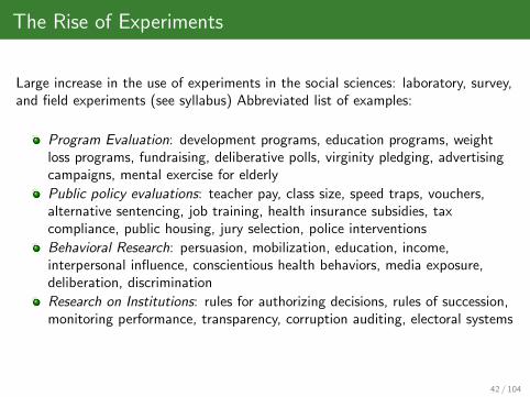
Large increase in the use of experiments in the social sciences: laboratory, survey,and field experiments (see syllabus) Abbreviated list of examples:
Program Evaluation: development programs, education programs, weightloss programs, fundraising, deliberative polls, virginity pledging, advertisingcampaigns, mental exercise for elderly
Public policy evaluations: teacher pay, class size, speed traps, vouchers,alternative sentencing, job training, health insurance subsidies, taxcompliance, public housing, jury selection, police interventions
Behavioral Research: persuasion, mobilization, education, income,interpersonal influence, conscientious health behaviors, media exposure,deliberation, discrimination
Research on Institutions: rules for authorizing decisions, rules of succession,monitoring performance, transparency, corruption auditing, electoral systems
39 / 104
The Rise of Experiments
Large increase in the use of experiments in the social sciences: laboratory, survey,and field experiments (see syllabus) Abbreviated list of examples:
Program Evaluation: development programs, education programs, weightloss programs, fundraising, deliberative polls, virginity pledging, advertisingcampaigns, mental exercise for elderly
Public policy evaluations: teacher pay, class size, speed traps, vouchers,alternative sentencing, job training, health insurance subsidies, taxcompliance, public housing, jury selection, police interventions
Behavioral Research: persuasion, mobilization, education, income,interpersonal influence, conscientious health behaviors, media exposure,deliberation, discrimination
Research on Institutions: rules for authorizing decisions, rules of succession,monitoring performance, transparency, corruption auditing, electoral systems
40 / 104
The Rise of Experiments
Large increase in the use of experiments in the social sciences: laboratory, survey,and field experiments (see syllabus) Abbreviated list of examples:
Program Evaluation: development programs, education programs, weightloss programs, fundraising, deliberative polls, virginity pledging, advertisingcampaigns, mental exercise for elderly
Public policy evaluations: teacher pay, class size, speed traps, vouchers,alternative sentencing, job training, health insurance subsidies, taxcompliance, public housing, jury selection, police interventions
Behavioral Research: persuasion, mobilization, education, income,interpersonal influence, conscientious health behaviors, media exposure,deliberation, discrimination
Research on Institutions: rules for authorizing decisions, rules of succession,monitoring performance, transparency, corruption auditing, electoral systems
41 / 104
The Rise of Experiments
Large increase in the use of experiments in the social sciences: laboratory, survey,and field experiments (see syllabus) Abbreviated list of examples:
Program Evaluation: development programs, education programs, weightloss programs, fundraising, deliberative polls, virginity pledging, advertisingcampaigns, mental exercise for elderly
Public policy evaluations: teacher pay, class size, speed traps, vouchers,alternative sentencing, job training, health insurance subsidies, taxcompliance, public housing, jury selection, police interventions
Behavioral Research: persuasion, mobilization, education, income,interpersonal influence, conscientious health behaviors, media exposure,deliberation, discrimination
Research on Institutions: rules for authorizing decisions, rules of succession,monitoring performance, transparency, corruption auditing, electoral systems
42 / 104
Outline
1 Hypothesis Testing in Small Samples
2 Using Covariates in Experiments
3 Examples
Social Pressure Experiment
Tax Compliance
Labor Market Discrimination
Job Training Partnership Act (JTPA)
4 Threats to Validity and Ethics
43 / 104
Social Pressure Experiment: Design
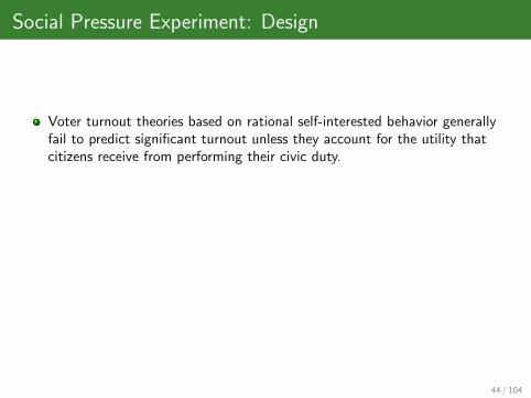
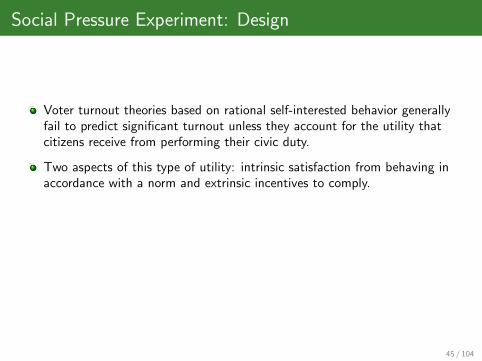
Voter turnout theories based on rational self-interested behavior generallyfail to predict significant turnout unless they account for the utility thatcitizens receive from performing their civic duty.
Two aspects of this type of utility: intrinsic satisfaction from behaving inaccordance with a norm and extrinsic incentives to comply.
Gerber, Green, and Larimer (2008) test these motives in a large scale fieldexperiment by applying varying degrees of intrinsic and extrinsic pressure onvoters using a series of mailings to 180,002 households before the August2006 primary election in Michigan.
44 / 104
Social Pressure Experiment: Design
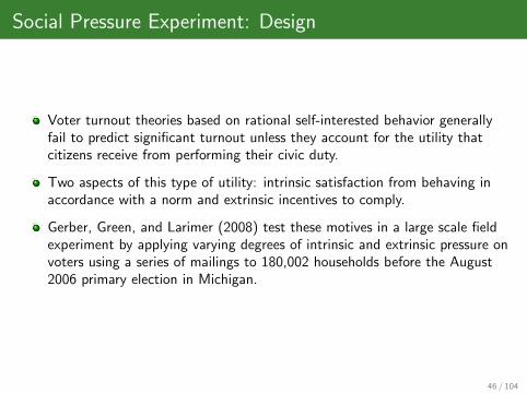
Voter turnout theories based on rational self-interested behavior generallyfail to predict significant turnout unless they account for the utility thatcitizens receive from performing their civic duty.
Two aspects of this type of utility: intrinsic satisfaction from behaving inaccordance with a norm and extrinsic incentives to comply.
Gerber, Green, and Larimer (2008) test these motives in a large scale fieldexperiment by applying varying degrees of intrinsic and extrinsic pressure onvoters using a series of mailings to 180,002 households before the August2006 primary election in Michigan.
45 / 104
Social Pressure Experiment: Design
Voter turnout theories based on rational self-interested behavior generallyfail to predict significant turnout unless they account for the utility thatcitizens receive from performing their civic duty.
Two aspects of this type of utility: intrinsic satisfaction from behaving inaccordance with a norm and extrinsic incentives to comply.
Gerber, Green, and Larimer (2008) test these motives in a large scale fieldexperiment by applying varying degrees of intrinsic and extrinsic pressure onvoters using a series of mailings to 180,002 households before the August2006 primary election in Michigan.
46 / 104
Social Pressure Experiment: Treatments
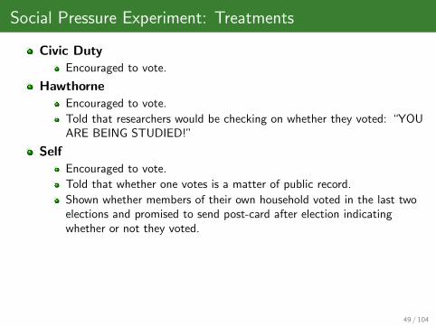
Civic DutyEncouraged to vote.
HawthorneEncouraged to vote.
Told that researchers would be checking on whether they voted: “YOUARE BEING STUDIED!”
SelfEncouraged to vote.
Told that whether one votes is a matter of public record.
Shown whether members of their own household voted in the last twoelections and promised to send post-card after election indicatingwhether or not they voted.
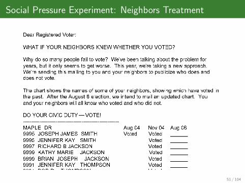
NeighborsLike Self treatment but in addition recipients are shown whether theneighbors on the block voted in the last two elections.
Promised to inform neighbors whether or not subject voted afterelection.
47 / 104
Social Pressure Experiment: Treatments
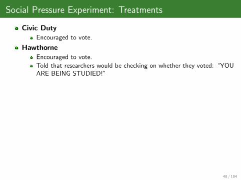
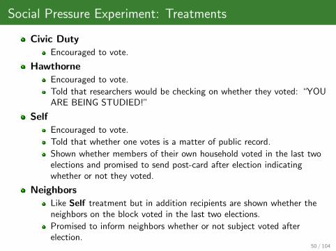
Civic DutyEncouraged to vote.
HawthorneEncouraged to vote.
Told that researchers would be checking on whether they voted: “YOUARE BEING STUDIED!”
SelfEncouraged to vote.
Told that whether one votes is a matter of public record.
Shown whether members of their own household voted in the last twoelections and promised to send post-card after election indicatingwhether or not they voted.
NeighborsLike Self treatment but in addition recipients are shown whether theneighbors on the block voted in the last two elections.
Promised to inform neighbors whether or not subject voted afterelection.
48 / 104
Social Pressure Experiment: Treatments
Civic DutyEncouraged to vote.
HawthorneEncouraged to vote.
Told that researchers would be checking on whether they voted: “YOUARE BEING STUDIED!”
SelfEncouraged to vote.
Told that whether one votes is a matter of public record.
Shown whether members of their own household voted in the last twoelections and promised to send post-card after election indicatingwhether or not they voted.
NeighborsLike Self treatment but in addition recipients are shown whether theneighbors on the block voted in the last two elections.
Promised to inform neighbors whether or not subject voted afterelection.
49 / 104
Social Pressure Experiment: Treatments
Civic DutyEncouraged to vote.
HawthorneEncouraged to vote.
Told that researchers would be checking on whether they voted: “YOUARE BEING STUDIED!”
SelfEncouraged to vote.
Told that whether one votes is a matter of public record.
Shown whether members of their own household voted in the last twoelections and promised to send post-card after election indicatingwhether or not they voted.
NeighborsLike Self treatment but in addition recipients are shown whether theneighbors on the block voted in the last two elections.
Promised to inform neighbors whether or not subject voted afterelection.
50 / 104
Social Pressure Experiment: Neighbors Treatment
Social Pressure and Voter Turnout February 2008
46
51 / 104
Social Pressure Experiment: Balance Check
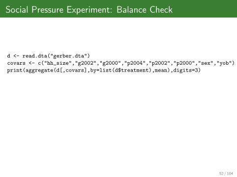
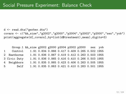
d <- read.dta("gerber.dta")
covars <- c("hh_size","g2002","g2000","p2004","p2002","p2000","sex","yob")
print(aggregate(d[,covars],by=list(d$treatment),mean),digits=3)
Group.1 hh_size g2002 g2000 p2004 p2002 p2000 sex yob
1 Control 1.91 0.834 0.866 0.417 0.409 0.265 0.502 1955
2 Hawthorne 1.91 0.836 0.867 0.419 0.412 0.263 0.503 1955
3 Civic Duty 1.91 0.836 0.865 0.416 0.410 0.266 0.503 1955
4 Neighbors 1.91 0.835 0.865 0.423 0.406 0.263 0.505 1955
5 Self 1.91 0.835 0.863 0.421 0.410 0.263 0.501 1955
52 / 104
Social Pressure Experiment: Balance Check
d <- read.dta("gerber.dta")
covars <- c("hh_size","g2002","g2000","p2004","p2002","p2000","sex","yob")
print(aggregate(d[,covars],by=list(d$treatment),mean),digits=3)
Group.1 hh_size g2002 g2000 p2004 p2002 p2000 sex yob
1 Control 1.91 0.834 0.866 0.417 0.409 0.265 0.502 1955
2 Hawthorne 1.91 0.836 0.867 0.419 0.412 0.263 0.503 1955
3 Civic Duty 1.91 0.836 0.865 0.416 0.410 0.266 0.503 1955
4 Neighbors 1.91 0.835 0.865 0.423 0.406 0.263 0.505 1955
5 Self 1.91 0.835 0.863 0.421 0.410 0.263 0.501 1955
53 / 104
Social Pressure Experiment: Balance Check
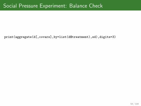
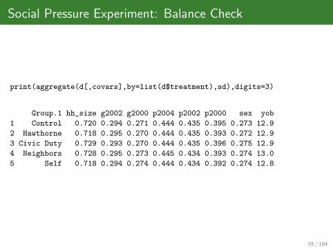
print(aggregate(d[,covars],by=list(d$treatment),sd),digits=3)
Group.1 hh_size g2002 g2000 p2004 p2002 p2000 sex yob
1 Control 0.720 0.294 0.271 0.444 0.435 0.395 0.273 12.9
2 Hawthorne 0.718 0.295 0.270 0.444 0.435 0.393 0.272 12.9
3 Civic Duty 0.729 0.293 0.270 0.444 0.435 0.396 0.275 12.9
4 Neighbors 0.728 0.295 0.273 0.445 0.434 0.393 0.274 13.0
5 Self 0.718 0.294 0.274 0.444 0.434 0.392 0.274 12.8
54 / 104
Social Pressure Experiment: Balance Check
print(aggregate(d[,covars],by=list(d$treatment),sd),digits=3)
Group.1 hh_size g2002 g2000 p2004 p2002 p2000 sex yob
1 Control 0.720 0.294 0.271 0.444 0.435 0.395 0.273 12.9
2 Hawthorne 0.718 0.295 0.270 0.444 0.435 0.393 0.272 12.9
3 Civic Duty 0.729 0.293 0.270 0.444 0.435 0.396 0.275 12.9
4 Neighbors 0.728 0.295 0.273 0.445 0.434 0.393 0.274 13.0
5 Self 0.718 0.294 0.274 0.444 0.434 0.392 0.274 12.8
55 / 104
Social Pressure Experiment: Balance Check
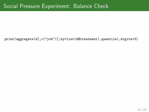
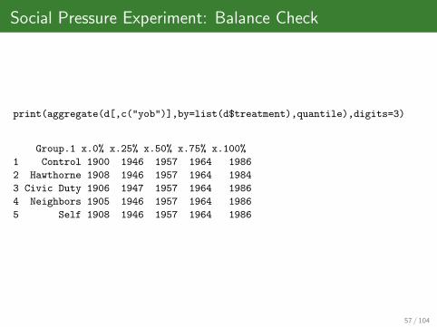
print(aggregate(d[,c("yob")],by=list(d$treatment),quantile),digits=3)
Group.1 x.0% x.25% x.50% x.75% x.100%
1 Control 1900 1946 1957 1964 1986
2 Hawthorne 1908 1946 1957 1964 1984
3 Civic Duty 1906 1947 1957 1964 1986
4 Neighbors 1905 1946 1957 1964 1986
5 Self 1908 1946 1957 1964 1986
56 / 104
Social Pressure Experiment: Balance Check
print(aggregate(d[,c("yob")],by=list(d$treatment),quantile),digits=3)
Group.1 x.0% x.25% x.50% x.75% x.100%
1 Control 1900 1946 1957 1964 1986
2 Hawthorne 1908 1946 1957 1964 1984
3 Civic Duty 1906 1947 1957 1964 1986
4 Neighbors 1905 1946 1957 1964 1986
5 Self 1908 1946 1957 1964 1986
57 / 104
Social Pressure Experiment: Multivariate Balance Check
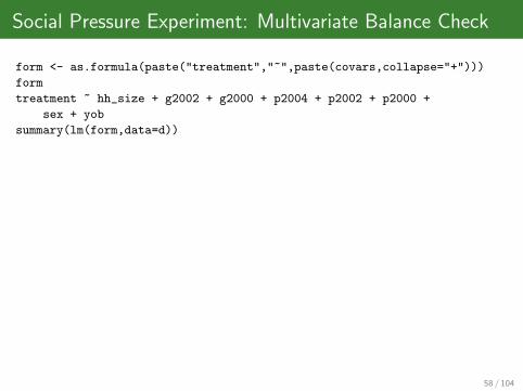
form <- as.formula(paste("treatment","~",paste(covars,collapse="+")))
form
treatment ~ hh_size + g2002 + g2000 + p2004 + p2002 + p2000 +
sex + yob
summary(lm(form,data=d))
Estimate Std. Error t value Pr(>|t|)
(Intercept) 1.7944614 0.5496699 3.265 0.0011 **
hh_size -0.0032727 0.0051836 -0.631 0.5278
g2002 0.0121818 0.0123389 0.987 0.3235
g2000 -0.0233410 0.0133489 -1.749 0.0804 .
p2004 0.0118147 0.0079130 1.493 0.1354
p2002 0.0018055 0.0081488 0.222 0.8247
p2000 -0.0031604 0.0087721 -0.360 0.7186
sex 0.0031331 0.0125052 0.251 0.8022
yob 0.0001671 0.0002815 0.594 0.5528
Residual standard error: 1.449 on 179993 degrees of freedom
Multiple R-squared: 4.004e-05, Adjusted R-squared: -4.406e-06
F-statistic: 0.9009 on 8 and 179993 DF, p-value: 0.5145
58 / 104
Social Pressure Experiment: Multivariate Balance Check
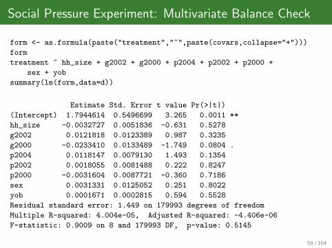
form <- as.formula(paste("treatment","~",paste(covars,collapse="+")))
form
treatment ~ hh_size + g2002 + g2000 + p2004 + p2002 + p2000 +
sex + yob
summary(lm(form,data=d))
Estimate Std. Error t value Pr(>|t|)
(Intercept) 1.7944614 0.5496699 3.265 0.0011 **
hh_size -0.0032727 0.0051836 -0.631 0.5278
g2002 0.0121818 0.0123389 0.987 0.3235
g2000 -0.0233410 0.0133489 -1.749 0.0804 .
p2004 0.0118147 0.0079130 1.493 0.1354
p2002 0.0018055 0.0081488 0.222 0.8247
p2000 -0.0031604 0.0087721 -0.360 0.7186
sex 0.0031331 0.0125052 0.251 0.8022
yob 0.0001671 0.0002815 0.594 0.5528
Residual standard error: 1.449 on 179993 degrees of freedom
Multiple R-squared: 4.004e-05, Adjusted R-squared: -4.406e-06
F-statistic: 0.9009 on 8 and 179993 DF, p-value: 0.5145
59 / 104
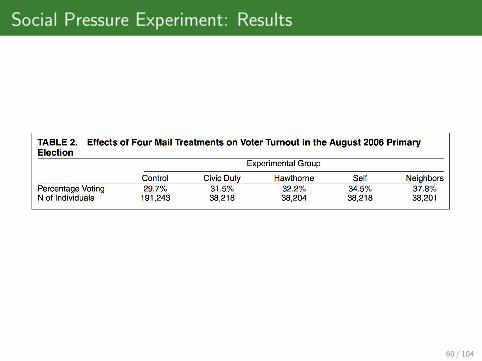
Social Pressure Experiment: Results
60 / 104
Social Pressure Experiment: Results
American Political Science Review Vol. 102, No. 1
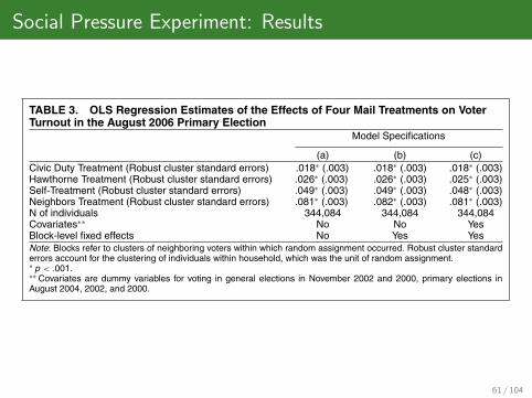
TABLE 3. OLS Regression Estimates of the Effects of Four Mail Treatments on VoterTurnout in the August 2006 Primary Election
Model Specifications
(a) (b) (c)Civic Duty Treatment (Robust cluster standard errors) .018∗ (.003) .018∗ (.003) .018∗ (.003)Hawthorne Treatment (Robust cluster standard errors) .026∗ (.003) .026∗ (.003) .025∗ (.003)Self-Treatment (Robust cluster standard errors) .049∗ (.003) .049∗ (.003) .048∗ (.003)Neighbors Treatment (Robust cluster standard errors) .081∗ (.003) .082∗ (.003) .081∗ (.003)N of individuals 344,084 344,084 344,084Covariates∗∗ No No YesBlock-level fixed effects No Yes YesNote: Blocks refer to clusters of neighboring voters within which random assignment occurred. Robust cluster standarderrors account for the clustering of individuals within household, which was the unit of random assignment.∗ p < .001.∗∗ Covariates are dummy variables for voting in general elections in November 2002 and 2000, primary elections inAugust 2004, 2002, and 2000.
randomized at the household-level is that proper esti-mation of the standard errors requires a correction forthe possibility that individuals within each householdshare unobserved characteristics (Arceneaux 2005).For this reason, Table 3 reports robust cluster stan-dard errors, which take intrahousehold correlation intoaccount. We also consider a range of different modelspecifications in order to gauge the robustness of theresults.
The first column of Table 3 reports the results of alinear regression in which voter turnout (Yi) for indi-vidual i is regressed on dummy variables D1i, D2i, D3i,D4i marking each of the four treatments (the refer-ence category is the control group). This model may bewritten simply as
Yi = β0 + β1D1i + β2D2i + β3D3i + β4D4i + ui, (6)
where ui represents an unobserved disturbance term.The second column embellishes this model by includingfixed effects C1i, C2i, . . . , C9999i for all but one of theK = 10,000 geographic clusters within which random-ization occurred:
Yi = β0 + β1D1i + β2D2i + β3D3i + β4D4i
+K−1∑
k=1
γkCki + ui. (7)
The parameters associated with these fixed effects areuninteresting for our purposes; we will focus on thetreatment parameters β1, β2, β3, and β4. The advantageof including fixed effects is the potential to eliminateany observed imbalances within each geographic clus-ter, thereby improving the precision of the estimates.The final column of Table 3 controls further for votingin five recent elections:
Yi = β0 + β1D1i + β2D2i + β3D3i + β4D4i +K−1∑
k=1
γkCki
+ λ1V1i + λ1V1i + · · · + λ5V5i + ui. (8)
Again, the point is to minimize disturbance varianceand improve the precision of the treatment estimates.
The results are remarkably robust, with scarcelyany movement even in the third decimal place.The average effect of the Civic Duty mailing is a1.8 percentage-point increase in turnout, suggestingthat priming civic duty has a measurable but not largeeffect on turnout. The Hawthorne mailing’s effect is2.5 percentage points. Mailings that list the household’sown voting record increase turnout by 4.8 percentagepoints, and including the voting behavior of neighborsraises the effect to 8.1 percentage points. All effectsare significant at p < .0001. Moreover, the Hawthornemailing is significantly more effective than the CivicDuty mailing ( p < .05, one-tailed); the Self mailingis significantly more effective than the Hawthornemailing ( p < .001); and the Neighbors mailing issignificantly more effective than the Self mailing( p < .001).
Having established that turnout increases marginallywhen civic duty is primed and dramatically when socialpressure is applied, the remaining question is whetherthe effects of social pressure interact with feelings ofcivic duty. Using an individual’s voting propensity asa proxy for the extent to which he or she feels anobligation to vote, we divided the observations intosix subsamples based on the number of votes cast infive prior elections; we further divided the subsamplesaccording to the number of voters in each household,because household size and past voting are correlated.As noted earlier, one hypothesis is that social pressureis particularly effective because it reinforces existingmotivation to participate. The contrary hypothesis isthat extrinsic incentives extinguish intrinsic motivation,resulting in greater treatment effects among those withlow voting propensities. To test these hypotheses whileat the same time taking into account floor and ceil-ing effects, we conducted a series of logistic regres-sions and examined the treatment effects across sub-groups.10 This analysis revealed that the treatment ef-fects on underlying voting propensities are more or
10 This analysis (not shown, but available on request) divided thesubjects according to past voting history and household size. Wetested the interaction hypothesis by means of a likelihood-ratio test,which failed to reject the null hypothesis of equal treatment effectsacross these subgroups.
39
61 / 104
Outline
1 Hypothesis Testing in Small Samples
2 Using Covariates in Experiments
3 Examples
Social Pressure Experiment
Tax Compliance
Labor Market Discrimination
Job Training Partnership Act (JTPA)
4 Threats to Validity and Ethics
62 / 104
Tax Compliance Experiment
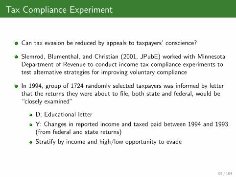
Can tax evasion be reduced by appeals to taxpayers’ conscience?
Slemrod, Blumenthal, and Christian (2001, JPubE) worked with MinnesotaDepartment of Revenue to conduct income tax compliance experiments totest alternative strategies for improving voluntary compliance
In 1994, group of 1724 randomly selected taxpayers was informed by letterthat the returns they were about to file, both state and federal, would be“closely examined”
D: Educational letter
Y: Changes in reported income and taxed paid between 1994 and 1993(from federal and state returns)
Stratify by income and high/low opportunity to evade
63 / 104
Tax Compliance Experiment
Can tax evasion be reduced by appeals to taxpayers’ conscience?
Slemrod, Blumenthal, and Christian (2001, JPubE) worked with MinnesotaDepartment of Revenue to conduct income tax compliance experiments totest alternative strategies for improving voluntary compliance
In 1994, group of 1724 randomly selected taxpayers was informed by letterthat the returns they were about to file, both state and federal, would be“closely examined”
D: Educational letter
Y: Changes in reported income and taxed paid between 1994 and 1993(from federal and state returns)
Stratify by income and high/low opportunity to evade
64 / 104
Tax Compliance Experiment
Can tax evasion be reduced by appeals to taxpayers’ conscience?
Slemrod, Blumenthal, and Christian (2001, JPubE) worked with MinnesotaDepartment of Revenue to conduct income tax compliance experiments totest alternative strategies for improving voluntary compliance
In 1994, group of 1724 randomly selected taxpayers was informed by letterthat the returns they were about to file, both state and federal, would be“closely examined”
D: Educational letter
Y: Changes in reported income and taxed paid between 1994 and 1993(from federal and state returns)
Stratify by income and high/low opportunity to evade
65 / 104
Tax Compliance Experiment
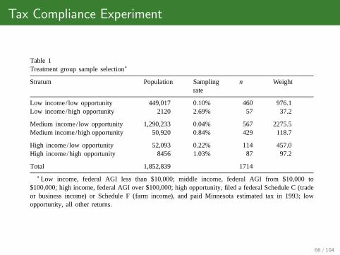
462 J. Slemrod et al. / Journal of Public Economics 79 (2001) 455 –483
Table 1aTreatment group sample selection
Stratum Population Sampling n Weightrate
Low income/ low opportunity 449,017 0.10% 460 976.1Low income/high opportunity 2120 2.69% 57 37.2
Medium income/ low opportunity 1,290,233 0.04% 567 2275.5Medium income/high opportunity 50,920 0.84% 429 118.7
High income/ low opportunity 52,093 0.22% 114 457.0High income/high opportunity 8456 1.03% 87 97.2
Total 1,852,839 1714a Low income, federal AGI less than $10,000; middle income, federal AGI from $10,000 to
$100,000; high income, federal AGI over $100,000; high opportunity, filed a federal Schedule C (tradeor business income) or Schedule F (farm income), and paid Minnesota estimated tax in 1993; lowopportunity, all other returns.
7but expected to have little reported income from their businesses. Taxpayers notin the high-opportunity category are referred to as low-opportunity.
The population count, sampling rate, and the resulting sample frequency foreach stratum are presented for the treatment group in Table 1 and for the control
8group in Table 2. Table 3 documents the further reduction in the sample by theelimination of returns (1) changing to, or from, married filing jointly, (2) filing fora different tax year, (3) not filing a 1994 tax return, or (4) having no positive
9income. This produced a working sample of 22,368 returns.
4.2. Experimental treatment
The treatment group received a letter by first-class mail from the Commissioner10of Revenue in January of 1995. Note that this treatment was administered after
the tax year, and at the beginning of the filing season. Thus, with a few exceptions(such as contributions to IRAs or Keoghs) it could not have affected non-reporting
7An advantage of a sample based on estimated-tax payers is the possibility of tailoring interventionsfor this group in the future if the experiment proved a success, because these taxpayers are involvedwith the department throughout the year. The low-opportunity group selected to represent the generalpopulation may provide valuable information about what approach to compliance works best withpeople who rarely would be the target of an audit.
8The control group from the ‘audit’ experiment was combined with the control group from the‘appeal to conscience’ experiment to increase precision. Both were randomly selected, and neither wascontacted by the Department of Revenue during the experiment.
9We also excluded a number of returns for which there was a single 1993 return associated with two1994 returns, presumably due to divorce.
10The letter was sent separately from the tax form itself, thus minimizing the possibility thattaxpayers who use professional preparers would discard the letter without reading it.
66 / 104
Tax Compliance Experiment
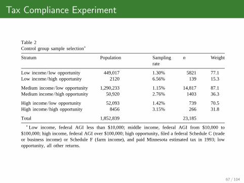
J. Slemrod et al. / Journal of Public Economics 79 (2001) 455 –483 463
Table 2aControl group sample selection
Stratum Population Sampling n Weightrate
Low income/ low opportunity 449,017 1.30% 5821 77.1Low income/high opportunity 2120 6.56% 139 15.3
Medium income/ low opportunity 1,290,233 1.15% 14,817 87.1Medium income/high opportunity 50,920 2.76% 1403 36.3
High income/ low opportunity 52,093 1.42% 739 70.5High income/high opportunity 8456 3.15% 266 31.8
Total 1,852,839 23,185a Low income, federal AGI less than $10,000; middle income, federal AGI from $10,000 to
$100,000; high income, federal AGI over $100,000; high opportunity, filed a federal Schedule C (tradeor business income) or Schedule F (farm income), and paid Minnesota estimated tax in 1993; lowopportunity, all other returns.
Table 3Excluded observations, by reason for exclusion and group status
Sample selection Treatment Control Total
1993 filers 1714 23,185 24,899Changed filing status 254 23.2% 2973 24.2% 21027Filed for different tax year 21 20.1% 27 0.0% 28Did not file 1994 federal return 2122 27.1% 21370 25.9% 21492No positive income 0.0% 24 0.0% 24
Total 1537 20,831 22,368
11behavior with tax consequences. The taxpayers were told: (1) that they had beenselected at random to be part of a study ‘that will increase the number of taxpayerswhose 1994 individual income tax returns are closely examined’; (2) that boththeir state and federal tax returns for the 1994 tax year would be closely examinedby the Minnesota Department of Revenue; (3) that they will be contacted aboutany discrepancies; and (4) that if any ‘irregularities’ were found, their returns filed
12in 1994 as well as prior years might be reviewed, as provided by law. The
11This aspect of the experiment is consistent with the Allingham and Sandmo (1972) assumption of afixed ‘true’ taxable income.
12The letter is not explicit about the penalties that would ensue if ‘irregularities’ were to bediscovered. Minnesota law provides for penalties of 20% of any ‘substantial’ understated tax, 10% ofany additional assessment due to negligence without intent to defraud and 50% of any extra taxassessed due to a fraudulent return. In addition, as a matter of course state tax enforcement agencieswould turn over what they’d learned to the IRS, and federal penalties would presumably apply, as well.
67 / 104
Results for Full Sample 466J.
Slemrod
etal.
/Journal
ofP
ublicE
conomics
79(2001)
455–483
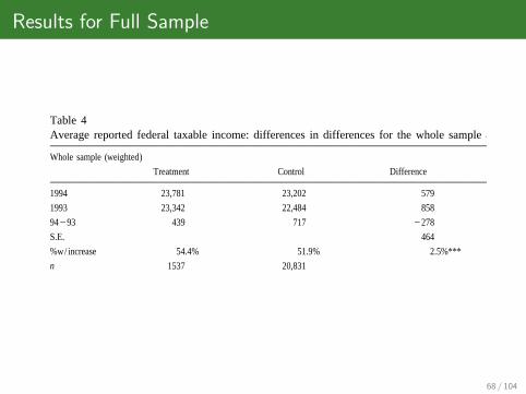
Table 4Average reported federal taxable income: differences in differences for the whole sample and income and opportunity groups
Whole sample (weighted)
Treatment Control Difference
1994 23,781 23,202 579
1993 23,342 22,484 858
94293 439 717 2278
S.E. 464
%w/increase 54.4% 51.9% 2.5%***
n 1537 20,831
Low income
High opportunity Low opportunity
Treatment Control Difference Treatment Control Difference
1994 7473 3992 3481 2397 2432 235
1993 971 787 183 788 942 2154**
94293 6502 3204 3298 1609 1490 119
S.E. 2718 189
%w/increase 65.4% 51.2% 14.2%* 52.2% 50.2% 2.0%
n 52 123 381 4829
68 / 104
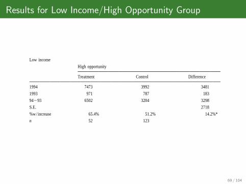
Results for Low Income/High Opportunity Group
466J.
Slemrod
etal.
/Journal
ofP
ublicE
conomics
79(2001)
455–483
Table 4Average reported federal taxable income: differences in differences for the whole sample and income and opportunity groups
Whole sample (weighted)
Treatment Control Difference
1994 23,781 23,202 579
1993 23,342 22,484 858
94293 439 717 2278
S.E. 464
%w/increase 54.4% 51.9% 2.5%***
n 1537 20,831
Low income
High opportunity Low opportunity
Treatment Control Difference Treatment Control Difference
1994 7473 3992 3481 2397 2432 235
1993 971 787 183 788 942 2154**
94293 6502 3204 3298 1609 1490 119
S.E. 2718 189
%w/increase 65.4% 51.2% 14.2%* 52.2% 50.2% 2.0%
n 52 123 381 4829
69 / 104
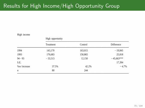
Results for High Income/High Opportunity Group
J.Slem
rodet
al./
Journalof
Public
Econom
ics79
(2001)455
–483467
Middle income
High opportunity Low opportunity
Treatment Control Difference Treatment Control Difference
1994 33,280 31,191 2089 24,316 23,669 646
1993 29,735 29,652 83 23,355 23,172 183
94293 3546 1539 2007 960 497 463
S.E. 1494 466
%w/increase 57.2% 53.1% 4.1% 56.0% 52.8% 3.2%
n 397 1318 520 13,636
High income
High opportunity Low opportunity
Treatment Control Difference Treatment Control Difference
1994 143,170 163,015 219,845 146,198 145,161 1037
1993 176,683 150,865 25,818 164,919 147,819 17,099
94293 233,513 12,150 245,663*** 218,721 22659 216,063
S.E. 17,394 10,455
%w/increase 37.5% 42.2% 24.7% 32.7% 43.6% 210.9%**
n 80 244 107 681
a *P,0.10; **P,0.05; ***P,0.01. Low income, federal AGI less than $10,000; middle income, federal AGI from $10,000 to $100,000; high income, federalAGI over $100,000; high opportunity, filed a federal Schedule C (trade or business income) or Schedule F (farm income), and paid Minnesota estimated tax in 1993;low opportunity, all other returns.
70 / 104
Outline
1 Hypothesis Testing in Small Samples
2 Using Covariates in Experiments
3 Examples
Social Pressure Experiment
Tax Compliance
Labor Market Discrimination
Job Training Partnership Act (JTPA)
4 Threats to Validity and Ethics
71 / 104
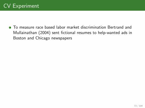
CV Experiment
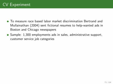
To measure race based labor market discrimination Bertrand andMullainathan (2004) sent fictional resumes to help-wanted ads inBoston and Chicago newspapers
Sample: 1,300 employments ads in sales, administrative support,customer service job categories
D: to manipulate perceived race, otherwise identical resumes arerandomly assigned African-American sounding names (Lakisha,Jamal, etc.) or White sounding names (Emily, Greg, etc.)
Four CVs are send to each ad (two high- and two low-qualityresumes, one of each CV is treatment/control)
Y: callback rates
72 / 104
CV Experiment
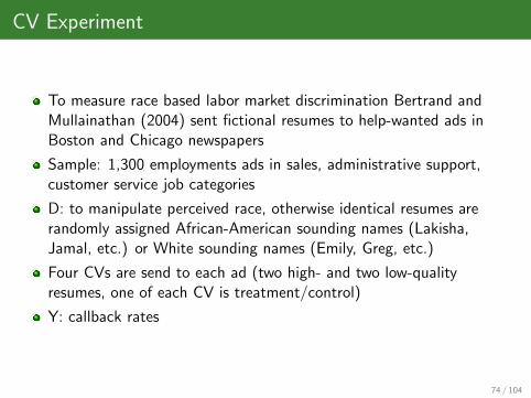
To measure race based labor market discrimination Bertrand andMullainathan (2004) sent fictional resumes to help-wanted ads inBoston and Chicago newspapers
Sample: 1,300 employments ads in sales, administrative support,customer service job categories
D: to manipulate perceived race, otherwise identical resumes arerandomly assigned African-American sounding names (Lakisha,Jamal, etc.) or White sounding names (Emily, Greg, etc.)
Four CVs are send to each ad (two high- and two low-qualityresumes, one of each CV is treatment/control)
Y: callback rates
73 / 104
CV Experiment
To measure race based labor market discrimination Bertrand andMullainathan (2004) sent fictional resumes to help-wanted ads inBoston and Chicago newspapers
Sample: 1,300 employments ads in sales, administrative support,customer service job categories
D: to manipulate perceived race, otherwise identical resumes arerandomly assigned African-American sounding names (Lakisha,Jamal, etc.) or White sounding names (Emily, Greg, etc.)
Four CVs are send to each ad (two high- and two low-qualityresumes, one of each CV is treatment/control)
Y: callback rates
74 / 104
Example: CV Experiment Results
VOL 94 NO. 4 BERTRAND AND MULLAINATHAN: RACE IN THE LABOR MARKET 997
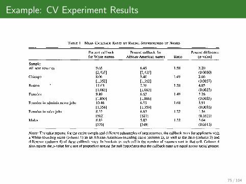
TABLE 1—MEAN CALLBACK RATES BY RACIAL SOUNDINGNESS OF NAMES
Sample:All sent resumes
Chicago
Boston '
Females
Females in administrative jobs
Females in sales jobs
Males
Percent callbackfor White names
9.65[2,435]8.06[1,352]11.63[1,083]9.89[1,860]10.46[1,358]8.37[502]8.87[575]
Percent callback forAfrican-American names
6.45[2,435]5.40[1,352]7.76[1,083]6.63[1,886]6.55[1,359]6.83[527]5.83[549]
Ratio
1.50
1.49
1.50
1.49
1.60
1.22
1.52
Percent difference(p-value)
3.20(0.0000)2.66(0.0057)4.05(0.0023)3.26(0.0003)3.91(0.0003)1.54(0.3523)3.04(0.0513)
Notes: The table reports, for the entire sample and different subsamples of sent resumes, the callback rates for applicants witha White-sounding name (column 1) an an African-American-sounding name (column 2), as well as the ratio (column 3) anddifference (column 4) of these callback rates. In brackets in each cell is the number of resumes sent in that cell. Column 4also reports the p-value for a test of proportion testing the null hypothesis that the callback rates are equal across racial groups.
employers rarely, if ever, contact applicants viapostal mail to set up interviews.
E. Weaknesses of the Experiment
We have already highlighted the strengths ofthis experiment relative to previous audit stud-ies. We now discuss its weaknesses. First, ouroutcome measure is crude, even relative to theprevious audit studies. Ultimately, one caresabout whether an applicant gets the job andabout the wage offered conditional on gettingthe job. Our procedure, however, simply mea-sures callbacks for interviews. To the extent thatthe search process has even moderate frictions,one would expect that reduced interview rateswould translate into reduced job offers. How-ever, we are not able to translate our results intogaps in hiring rates or gaps in earnings.
Another weakness is that the resumes do notdirectly report race but instead suggest racethrough personal names. This leads to varioussources of concern. First, while the names arechosen to make race salient, some employersmay simply not notice the names or not recog-nize their racial content. On a related note,because we are not assigning race but onlyrace-specific names, our results are not repre-sentative of the average African-American(who may not have such a racially distinct
^ We return to this issue in Section IV,subsection B.
Finally, and this is an issue pervasive in bothour study and the pair-matching audit studies,newspaper ads represent only one channel forjob search. As is well known from previouswork, social networks are another commonmeans through which people find jobs and onethat clearly cannot be studied here. This omis-sion could qualitatively affect our results ifAfrican-Americans use social networks more orif employers who rely more on networks differ-entiate less by race.29
III. Results
A. Is There a Racial Gap in Callback?
Table 1 tabulates average callback rates byracial soundingness of names. Included inbrackets under each rate is the number of re-sumes sent in that cell. Row 1 presents ourresults for the full data set. Resumes with White
'' As Appendix Table Al indicates, the African-American names we use are, however, quite commonamong African-Americans, making this less of a concern.
* In fact, there is some evidence that African-Americansmay rely less on social networks for their job search (HarryJ. Holzer, 1987).
75 / 104
Outline
1 Hypothesis Testing in Small Samples
2 Using Covariates in Experiments
3 Examples
Social Pressure Experiment
Tax Compliance
Labor Market Discrimination
Job Training Partnership Act (JTPA)
4 Threats to Validity and Ethics
76 / 104
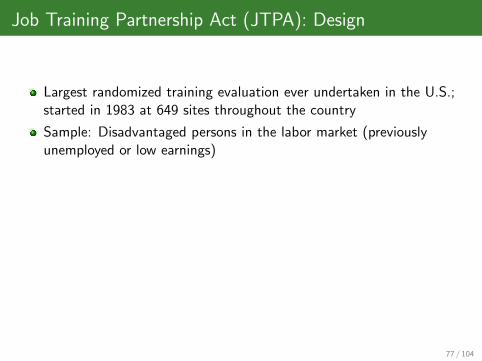
Job Training Partnership Act (JTPA): Design
Largest randomized training evaluation ever undertaken in the U.S.;started in 1983 at 649 sites throughout the country
Sample: Disadvantaged persons in the labor market (previouslyunemployed or low earnings)
D: Assignment to one of three general service strategies
classroom training in occupational skillson-the-job training and/or job search assistanceother services (eg. probationary employment)
Y: Earnings 30 months following assignment
X: Characteristics measured before assignment (age, gender, previousearnings, race, etc.)
77 / 104
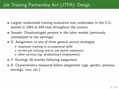
Job Training Partnership Act (JTPA): Design
Largest randomized training evaluation ever undertaken in the U.S.;started in 1983 at 649 sites throughout the country
Sample: Disadvantaged persons in the labor market (previouslyunemployed or low earnings)
D: Assignment to one of three general service strategies
classroom training in occupational skillson-the-job training and/or job search assistanceother services (eg. probationary employment)
Y: Earnings 30 months following assignment
X: Characteristics measured before assignment (age, gender, previousearnings, race, etc.)
78 / 104
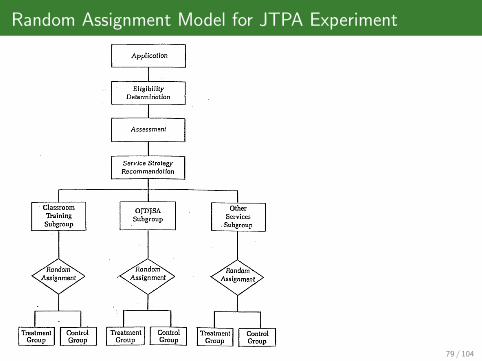
Random Assignment Model for JTPA Experiment
79 / 104
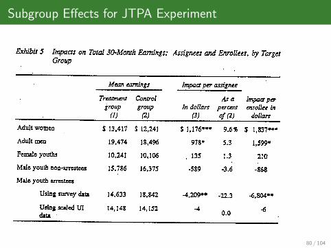
Subgroup Effects for JTPA Experiment
80 / 104
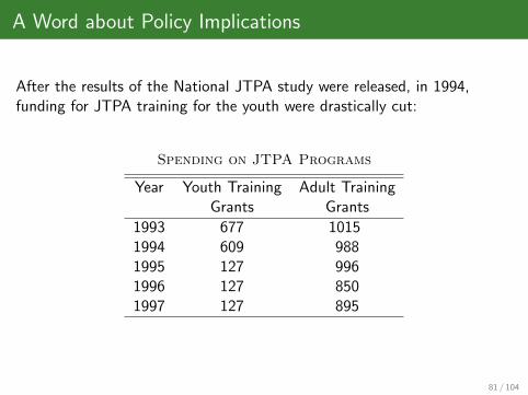
A Word about Policy Implications
After the results of the National JTPA study were released, in 1994,funding for JTPA training for the youth were drastically cut:
Spending on JTPA Programs
Year Youth Training Adult TrainingGrants Grants
1993 677 10151994 609 9881995 127 9961996 127 8501997 127 895
81 / 104
Outline
1 Hypothesis Testing in Small Samples
2 Using Covariates in Experiments
3 Examples
Social Pressure Experiment
Tax Compliance
Labor Market Discrimination
Job Training Partnership Act (JTPA)
4 Threats to Validity and Ethics
82 / 104
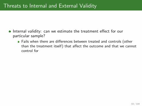
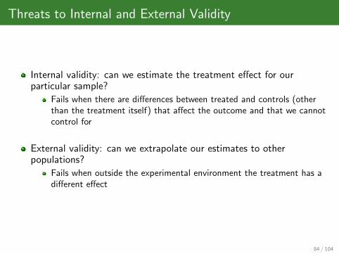
Threats to Internal and External Validity
Internal validity: can we estimate the treatment effect for ourparticular sample?
Fails when there are differences between treated and controls (otherthan the treatment itself) that affect the outcome and that we cannotcontrol for
External validity: can we extrapolate our estimates to otherpopulations?
Fails when outside the experimental environment the treatment has adifferent effect
83 / 104
Threats to Internal and External Validity
Internal validity: can we estimate the treatment effect for ourparticular sample?
Fails when there are differences between treated and controls (otherthan the treatment itself) that affect the outcome and that we cannotcontrol for
External validity: can we extrapolate our estimates to otherpopulations?
Fails when outside the experimental environment the treatment has adifferent effect
84 / 104
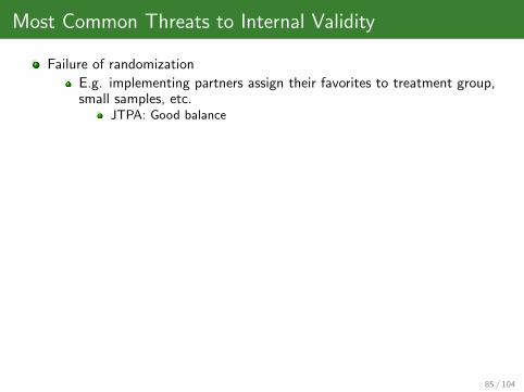
Most Common Threats to Internal Validity
Failure of randomization
E.g. implementing partners assign their favorites to treatment group,small samples, etc.
JTPA: Good balance
Non-compliance with experimental protocol
Failure to treat or “crossover”: Some members of the control groupreceive the treatment and some in the treatment group go untreatedCan reduce power significantly
JTPA: only about 65% of those assigned to treatment actually enrolledin training (compliance was almost perfect in the control group)
Attrition
Can destroy validity if observed potential outcomes are notrepresentative of all potential outcomes even with randomizationE.g. control group subjects are more likely to drop out of a study
JTPA: only 3 percent dropped out
Spillovers
Should be dealt with in the design
85 / 104

Most Common Threats to Internal Validity
Failure of randomization
E.g. implementing partners assign their favorites to treatment group,small samples, etc.
JTPA: Good balance
Non-compliance with experimental protocol
Failure to treat or “crossover”: Some members of the control groupreceive the treatment and some in the treatment group go untreatedCan reduce power significantly
JTPA: only about 65% of those assigned to treatment actually enrolledin training (compliance was almost perfect in the control group)
Attrition
Can destroy validity if observed potential outcomes are notrepresentative of all potential outcomes even with randomizationE.g. control group subjects are more likely to drop out of a study
JTPA: only 3 percent dropped out
Spillovers
Should be dealt with in the design
86 / 104
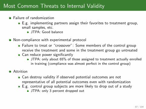
Most Common Threats to Internal Validity
Failure of randomization
E.g. implementing partners assign their favorites to treatment group,small samples, etc.
JTPA: Good balance
Non-compliance with experimental protocol
Failure to treat or “crossover”: Some members of the control groupreceive the treatment and some in the treatment group go untreatedCan reduce power significantly
JTPA: only about 65% of those assigned to treatment actually enrolledin training (compliance was almost perfect in the control group)
Attrition
Can destroy validity if observed potential outcomes are notrepresentative of all potential outcomes even with randomizationE.g. control group subjects are more likely to drop out of a study
JTPA: only 3 percent dropped out
Spillovers
Should be dealt with in the design
87 / 104
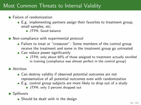
Most Common Threats to Internal Validity
Failure of randomization
E.g. implementing partners assign their favorites to treatment group,small samples, etc.
JTPA: Good balance
Non-compliance with experimental protocol
Failure to treat or “crossover”: Some members of the control groupreceive the treatment and some in the treatment group go untreatedCan reduce power significantly
JTPA: only about 65% of those assigned to treatment actually enrolledin training (compliance was almost perfect in the control group)
Attrition
Can destroy validity if observed potential outcomes are notrepresentative of all potential outcomes even with randomizationE.g. control group subjects are more likely to drop out of a study
JTPA: only 3 percent dropped out
Spillovers
Should be dealt with in the design88 / 104
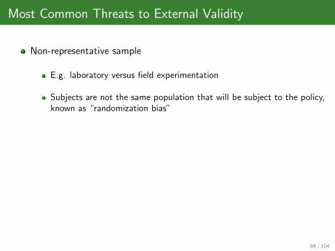
Most Common Threats to External Validity
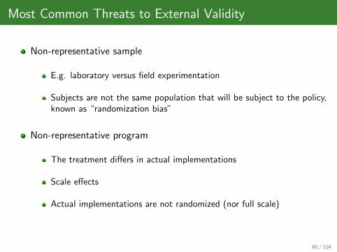
Non-representative sample
E.g. laboratory versus field experimentation
Subjects are not the same population that will be subject to the policy,known as “randomization bias”
Non-representative program
The treatment differs in actual implementations
Scale effects
Actual implementations are not randomized (nor full scale)
89 / 104
Most Common Threats to External Validity
Non-representative sample
E.g. laboratory versus field experimentation
Subjects are not the same population that will be subject to the policy,known as “randomization bias”
Non-representative program
The treatment differs in actual implementations
Scale effects
Actual implementations are not randomized (nor full scale)
90 / 104
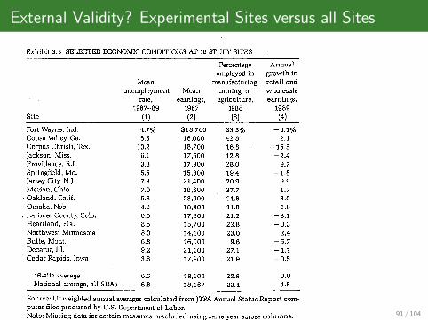
External Validity? Experimental Sites versus all Sites
91 / 104
Internal vs. External Validity
Which one is more important?
One common view is that internal validity comes first. If youdo not know the effects of the treatment on the units in yourstudy, you are not well-positioned to infer the effects on unitsyou did not study who live in circumstances you did notstudy. (Rosenbaum 2010, p. 56)
Randomization addresses internal validity. External validity is oftenaddressed by comparing the results of several internally valid studiesconducted in different circumstances and at different times.
The same issues apply in observational studies.
92 / 104
Internal vs. External Validity
Which one is more important?
One common view is that internal validity comes first. If youdo not know the effects of the treatment on the units in yourstudy, you are not well-positioned to infer the effects on unitsyou did not study who live in circumstances you did notstudy. (Rosenbaum 2010, p. 56)
Randomization addresses internal validity. External validity is oftenaddressed by comparing the results of several internally valid studiesconducted in different circumstances and at different times.
The same issues apply in observational studies.
93 / 104

Hardwork is in the Design and Implementation
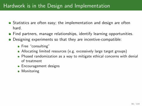
Statistics are often easy; the implementation and design are oftenhard.
Find partners, manage relationships, identify learning opportunities.
Designing experiments so that they are incentive-compatible:
Free “consulting”
Allocating limited resources (e.g. excessively large target groups)
Phased randomization as a way to mitigate ethical concerns with denialof treatment
Encouragement designs
Monitoring
Potentially high costs.
Many things can go wrong with complex and large scale experiments.
Keep it simple in the field!
94 / 104

Hardwork is in the Design and Implementation
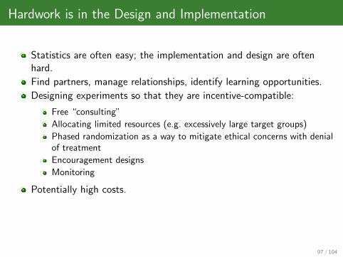
Statistics are often easy; the implementation and design are oftenhard.
Find partners, manage relationships, identify learning opportunities.
Designing experiments so that they are incentive-compatible:
Free “consulting”
Allocating limited resources (e.g. excessively large target groups)
Phased randomization as a way to mitigate ethical concerns with denialof treatment
Encouragement designs
Monitoring
Potentially high costs.
Many things can go wrong with complex and large scale experiments.
Keep it simple in the field!
95 / 104
Hardwork is in the Design and Implementation
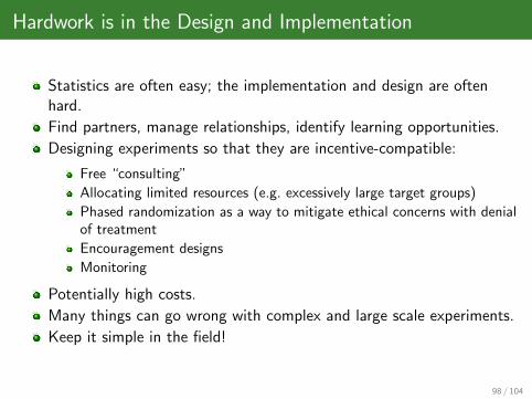
Statistics are often easy; the implementation and design are oftenhard.
Find partners, manage relationships, identify learning opportunities.
Designing experiments so that they are incentive-compatible:
Free “consulting”
Allocating limited resources (e.g. excessively large target groups)
Phased randomization as a way to mitigate ethical concerns with denialof treatment
Encouragement designs
Monitoring
Potentially high costs.
Many things can go wrong with complex and large scale experiments.
Keep it simple in the field!
96 / 104
Hardwork is in the Design and Implementation
Statistics are often easy; the implementation and design are oftenhard.
Find partners, manage relationships, identify learning opportunities.
Designing experiments so that they are incentive-compatible:
Free “consulting”
Allocating limited resources (e.g. excessively large target groups)
Phased randomization as a way to mitigate ethical concerns with denialof treatment
Encouragement designs
Monitoring
Potentially high costs.
Many things can go wrong with complex and large scale experiments.
Keep it simple in the field!
97 / 104
Hardwork is in the Design and Implementation
Statistics are often easy; the implementation and design are oftenhard.
Find partners, manage relationships, identify learning opportunities.
Designing experiments so that they are incentive-compatible:
Free “consulting”
Allocating limited resources (e.g. excessively large target groups)
Phased randomization as a way to mitigate ethical concerns with denialof treatment
Encouragement designs
Monitoring
Potentially high costs.
Many things can go wrong with complex and large scale experiments.
Keep it simple in the field!
98 / 104
Ethics and Experimentation
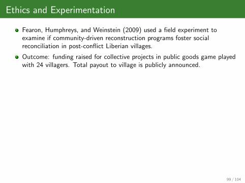
Fearon, Humphreys, and Weinstein (2009) used a field experiment toexamine if community-driven reconstruction programs foster socialreconciliation in post-conflict Liberian villages.
Outcome: funding raised for collective projects in public goods game playedwith 24 villagers. Total payout to village is publicly announced.
We received a report that leaders in one community had gatheredvillagers together after we left and asked people to report how muchthey had contributed. We moved quickly to prevent any retributionin that village, but also decided to alter the protocol for subsequentgames to ensure greater protection for game participants.
These changes included stronger language about the importance ofprotecting anonymity, random audits of community behavior,facilitation of anonymous reporting of violations of game protocol byparticipants, and a new opportunity to receive supplemental fundsin a postproject lottery if no reports of harassment were received.
99 / 104
Ethics and Experimentation
Fearon, Humphreys, and Weinstein (2009) used a field experiment toexamine if community-driven reconstruction programs foster socialreconciliation in post-conflict Liberian villages.
Outcome: funding raised for collective projects in public goods game playedwith 24 villagers. Total payout to village is publicly announced.
We received a report that leaders in one community had gatheredvillagers together after we left and asked people to report how muchthey had contributed. We moved quickly to prevent any retributionin that village, but also decided to alter the protocol for subsequentgames to ensure greater protection for game participants.
These changes included stronger language about the importance ofprotecting anonymity, random audits of community behavior,facilitation of anonymous reporting of violations of game protocol byparticipants, and a new opportunity to receive supplemental fundsin a postproject lottery if no reports of harassment were received.
100 / 104
Ethics and Experimentation
Fearon, Humphreys, and Weinstein (2009) used a field experiment toexamine if community-driven reconstruction programs foster socialreconciliation in post-conflict Liberian villages.
Outcome: funding raised for collective projects in public goods game playedwith 24 villagers. Total payout to village is publicly announced.
We received a report that leaders in one community had gatheredvillagers together after we left and asked people to report how muchthey had contributed. We moved quickly to prevent any retributionin that village, but also decided to alter the protocol for subsequentgames to ensure greater protection for game participants.
These changes included stronger language about the importance ofprotecting anonymity, random audits of community behavior,facilitation of anonymous reporting of violations of game protocol byparticipants, and a new opportunity to receive supplemental fundsin a postproject lottery if no reports of harassment were received.
101 / 104
Ethics and Experimentation
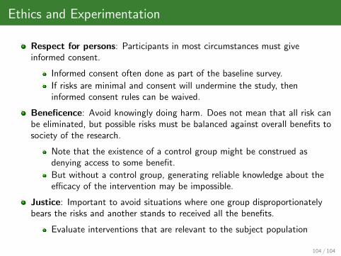
Respect for persons: Participants in most circumstances must giveinformed consent.
Informed consent often done as part of the baseline survey.
If risks are minimal and consent will undermine the study, theninformed consent rules can be waived.
Beneficence: Avoid knowingly doing harm. Does not mean that all risk canbe eliminated, but possible risks must be balanced against overall benefits tosociety of the research.
Note that the existence of a control group might be construed asdenying access to some benefit.
But without a control group, generating reliable knowledge about theefficacy of the intervention may be impossible.
Justice: Important to avoid situations where one group disproportionatelybears the risks and another stands to received all the benefits.
Evaluate interventions that are relevant to the subject population
102 / 104
Ethics and Experimentation
Respect for persons: Participants in most circumstances must giveinformed consent.
Informed consent often done as part of the baseline survey.
If risks are minimal and consent will undermine the study, theninformed consent rules can be waived.
Beneficence: Avoid knowingly doing harm. Does not mean that all risk canbe eliminated, but possible risks must be balanced against overall benefits tosociety of the research.
Note that the existence of a control group might be construed asdenying access to some benefit.
But without a control group, generating reliable knowledge about theefficacy of the intervention may be impossible.
Justice: Important to avoid situations where one group disproportionatelybears the risks and another stands to received all the benefits.
Evaluate interventions that are relevant to the subject population
103 / 104
Ethics and Experimentation
Respect for persons: Participants in most circumstances must giveinformed consent.
Informed consent often done as part of the baseline survey.
If risks are minimal and consent will undermine the study, theninformed consent rules can be waived.
Beneficence: Avoid knowingly doing harm. Does not mean that all risk canbe eliminated, but possible risks must be balanced against overall benefits tosociety of the research.
Note that the existence of a control group might be construed asdenying access to some benefit.
But without a control group, generating reliable knowledge about theefficacy of the intervention may be impossible.
Justice: Important to avoid situations where one group disproportionatelybears the risks and another stands to received all the benefits.
Evaluate interventions that are relevant to the subject population
104 / 104
Ethics and Experimentation
IRB approval is required in almost all circumstances.
If running an experiment in another country, you need to follow the localregulations on experimental research.
Often poorly adapted to social science.Or legally murky whether or not approval is required.
Still many unanswered questions and lack of consensus on the ethics of fieldexperimentation within the social sciences!
Be prepared to confront wildly varying opinions on these issues.
105 / 104