Embed Size (px)
Citation preview
Part 1: A Theoretical and Practical Introduction to SPARROW 69
1.5.2.2 Asymptotic properties within a single basin—three examples (advanced)
In an attempt to establish consistency and asymptotic normality for the SPARROW model parameter estimates, we immediately encounter a technical problem. The problem arises in the assumptions needed to extend the number of observations to an infinitely large size. In many applications of a SPARROW model, the researcher will have a prescribed watershed containing a defined reach network. Because the watershed represents a bounded region, the only way in which observations can be extended to infinity is by infilling—that is, increasing the density of measurements within the study area. A hydrologic system is by nature bounded and accumulative, however, meaning the contaminant flux at the outflow of the basin is an accumulation of individual processes within a bounded watershed. It is also true that not all uncertainty in the description of the basin can be resolved at the basin outlet, even if the uncertainty is independent at the smallest scale. As is shown below, the existence of error at the aggregate scale implies asymptotic theory commonly used to justify finite sample estimates is not valid in the context of a finite watershed.
To better understand the limitations imposed by a finite basin with aggregate error, we present three examples. Each example is built from a stochastic process that is well defined and statistically independent at the smallest scale, yet leads to non-degenerate stochastic behavior at the aggregate scale. The examples demonstrate that model estimates from finite basins do not converge in probability to a constant, implying the asymptotic properties of consistency and normality do not necessarily hold. The utility of this result is technical; however, the examples serve another purpose—they demonstrate how a SPARROW model arises from a fundamental description of hydrologic stochastic processes. In this way, some light is shed on the somewhat ‘black box’ nature of large-scale hydrologic models.
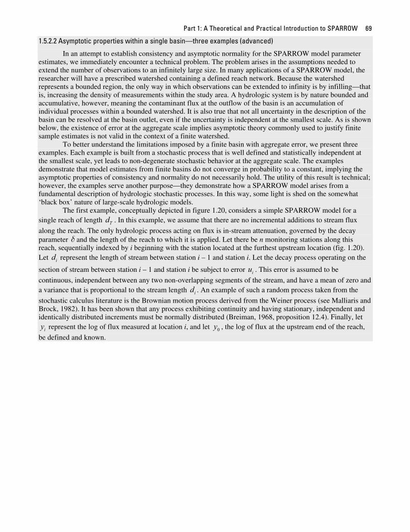
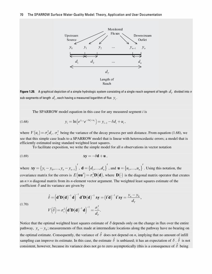
The first example, conceptually depicted in figure 1.20, considers a simple SPARROW model for a single reach of length . In this example, we assume that there are no incremental additions to stream flux Tdalong the reach. The only hydrologic process acting on flux is in-stream attenuation, governed by the decay parameter δ and the length of the reach to which it is applied. Let there be n monitoring stations along this reach, sequentially indexed by i beginning with the station located at the furthest upstream location (fig. 1.20). Let represent the length of stream between station i – 1 and station i. Let the decay process operating on the idsection of stream between station i – 1 and station i be subject to error . This error is assumed to be iucontinuous, independent between any two non-overlapping segments of the stream, and have a mean of zero and a variance that is proportional to the stream length . An example of such a random process taken from the idstochastic calculus literature is the Brownian motion process derived from the Weiner process (see Malliaris and Brock, 1982). It has been shown that any process exhibiting continuity and having stationary, independent and identically distributed increments must be normally distributed (Breiman, 1968, proposition 12.4). Finally, let
iy represent the log of flux measured at location i, and let 0y , the log of flux at the upstream end of the reach,
be defined and known.
The SPARROW Surface Water-Quality Model: Theory, Application and User Documentation 70
Figure 1.20. A graphical depiction of a simple hydrologic system consisting of a single reach segment of length divided into n Tdsub-segments of length , each having a measured logarithm of flux id iy .
The SPARROW model equation in this case for any measured segment i is
(1.68) ( )11ln i i iy d u
i iy e e y dδ δ− − +−= = − i iu+ ,
where ( ) 2i v iV u , being the variance of the decay process per unit distance. From equation (1.68), we dσ= 2
vσsee that this simple case leads to a SPARROW model that is linear with heteroscedastic errors; a model that is efficiently estimated using standard weighted least squares.
To facilitate exposition, we write the simple model for all n observations in vector notation
(1.69) , δ=− +Δy d u
where Δ , , and . Using this notation, the { }1 0 1, , n ny y y y −′
= − −y … { }1, , nd d ′=d … }{ 1, , nu u ′
=u …
covariance matrix for the errors is ( ) ( )2vE σ′ =uu D d , where is the diagonal matrix operator that creates ( )⋅D
an n×n diagonal matrix from its n-element vector argument. The weighted least squares estimate of the coefficient δ and its variance are given by
(1.70)
( )( ) ( ) ( )
( ) ( )( )
1 11 1 0
2112
ˆ ,
ˆ .
n
T
vv
T
y yd
Vd
δ
σδ σ
− −− −
−−
−′ ′ ′ ′= =
′= =
Δ Δd D d d d D d y i d i y
d D d d
=
Notice that the optimal weighted least squares estimate of δ depends only on the change in flux over the entire pathway, 0ny y− ; measurements of flux made at intermediate locations along the pathway have no bearing on
the optimal estimate. Consequently, the variance of does not depend on n, implying that no amount of infill δsampling can improve its estimate. In this case, the estimate is unbiased; it has an expectation of δ . is not δ δconsistent, however, because its variance does not go to zero asymptotically (this is a consequence of being δ
Part 1: A Theoretical and Practical Introduction to SPARROW 71
normally distributed; see theorem 18.14 in Davidson, 1994). Here, because are derived from a Wiener iu
process, the distribution of will be normal. It is possible, however, to construct other examples in which the δunderlying process is not continuous, and therefore not Wiener and not normally distributed. Consequently, the asymptotic distribution of the estimated decay rate need not be normal.
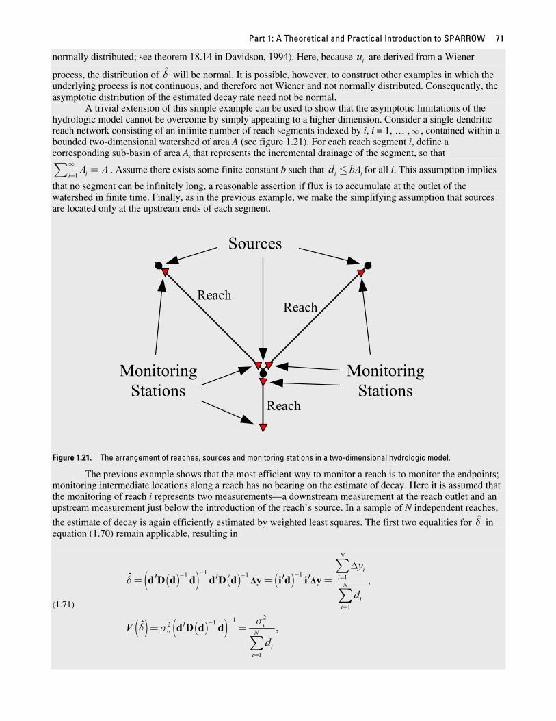
A trivial extension of this simple example can be used to show that the asymptotic limitations of the hydrologic model cannot be overcome by simply appealing to a higher dimension. Consider a single dendritic reach network consisting of an infinite number of reach segments indexed by i, i = 1, … , , contained within a ∞bounded two-dimensional watershed of area A (see figure 1.21). For each reach segment i, define a corresponding sub-basin of area Ai that represents the incremental drainage of the segment, so that
1 iiA A∞
==∑ i. Assume there exists some finite constant b such that for all i. This assumption implies id bA≤
that no segment can be infinitely long, a reasonable assertion if flux is to accumulate at the outlet of the watershed in finite time. Finally, as in the previous example, we make the simplifying assumption that sources are located only at the upstream ends of each segment.
Sources
Monitoring Stations
Monitoring Stations
ReachReach
Reach
Figure 1.21. The arrangement of reaches, sources and monitoring stations in a two-dimensional hydrologic model.
The previous example shows that the most efficient way to monitor a reach is to monitor the endpoints; monitoring intermediate locations along a reach has no bearing on the estimate of decay. Here it is assumed that the monitoring of reach i represents two measurements—a downstream measurement at the reach outlet and an upstream measurement just below the introduction of the reach’s source. In a sample of N independent reaches,
the estimate of decay is again efficiently estimated by weighted least squares. The first two equalities for in δequation (1.70) remain applicable, resulting in
(1.71)
( )( ) ( ) ( )
( ) ( )( )
1 11 1 1
1
2112
1
ˆ ,
ˆ ,
N
iiN
ii
vv N
ii
y
d
Vd
δ
σδ σ
− −− − =
=
−−
=
Δ
′ ′ ′ ′= =
′= =
∑
∑
∑
Δ Δd D d d d D d y i d i y
d D d d
=
The SPARROW Surface Water-Quality Model: Theory, Application and User Documentation 72
where, in this context, the ith element of pertains to the difference between the downstream and upstream Δy
measurements of reach i. Since for each i, we have id bA≤ i
(1.72) ( )2 2
1
ˆ v vN
ii
VbAb A
σ σδ
=
> ≥∑
.
The variance of the estimator is again bounded away from zero, regardless of the number of observations. As N
goes to infinity, and every segment of the reach network becomes monitored, the variance of does not go to δzero. Consequently, the conditions for consistency are not met.
The last example demonstrates that the limitations of asymptotic analysis within a finite basin are not restricted to the estimation of the decay rate, but also pertain to the estimation of source coefficients. Consider again the simple case of a single reach of length . For this example, it is assumed that the in-stream decay Tdrate is zero throughout the full reach segment. Arrayed along the reach segment are sources, defined
continuously by the function . Associated with each source is a source coefficient that determines the ( )S t
amount of source that is delivered to the stream. The source coefficient is assumed to be stochastic and is ( )S t
given by ( )( )a dq t , where a is a constant and dq(t) is a Poisson jump process defined over continuous distance
t, where dq(t) equals 1 with probability λdt and equals zero with probability 1 (see Malliaris and Brock, dtλ−1982). Thus, the expectation of dq(t) is λdt, and the variance is (ignoring terms smaller than dt) also λdt. The adoption of a Poisson process to define the source coefficient implies sources are effectively distributed discretely over the length of the reach but can occur at any location with equal probability. Because q(t) has jumps, it is not a continuous process, as was the case for the Wiener process used in the examples involving stream decay. Like a Wiener process, however, the Poisson process q(t) has the Markov property that the probability distribution for all downstream values of the q(t + s) conditioned on all information available at location t depends only on the local value of q(t) and not on any upstream values. This implies the intervals dq(t) and dq(s) are independent for . s t≠
Assume monitoring stations are positioned at locations , with spacing . The , 1, ,it i n= … 1i i id t t −= −flux measured at station i is given by
(1.73) ( )1
1
1 ( )
i i
i
t d
i i tY Y a S t dq t
−
−
+
−= + ∫ .
The mean and variance of are given by 1i iY Y−−
(1.74) ( ) (1
1
1
i i
i
t d
i i tE Y Y a S t dtλ
−
−
+
−− = )∫ , and
(1.75) ( ) ( )1
1
2 2
1
i i
i
t d
i i tV Y Y a S t dtλ
−
−
+
−− = ∫ .
Due to the assumptions associated with q(t), the covariance between and 1i iY Y−− 1j jY Y −− is zero for i j . ≠
Estimates of the source coefficient a and Poisson parameter λ can be obtained from a simple linear model having the form (1.76) , b= +ΔY X Z
Part 1: A Theoretical and Practical Introduction to SPARROW 73
where , { }1 2 1 1, , , n nY Y Y Y Y −′
= − −ΔY … ( ) ( ) ( ){ }1 1 2 1
1 1
0 , , ,
n n
n
d t d t d
t tS t dt S t dt S t dt
−
−
+ + ′= ∫ ∫ ∫X … , , b aλ=
and error vector { 1, , n}Z Z ′=Z … has zero mean and diagonal covariance matrix , with D(g) being a ( )2a λD g
diagonal matrix having diagonal elements g given by the vector
( ) ( ) ( ){ }1 1 2 1
1 1
2 2 2
0 , , ,
n n
n
d t d t d
t tS t dt S t dt S t dt
−
−
+ + ′= ∫ ∫ ∫g … . The model given in equation (1.76) is not
technically a SPARROW model because it is estimated in real space as opposed to logarithm space, but it is a valid model and will suffice to make the necessary point concerning asymptotic properties of estimators based on infinitely dense monitoring stations.
Equation (1.76) can be estimated using linear weighted least squares, with the weight of observation i
set to ( )1
1
2
1
i i
i
t d
tS t dt
−
−
+
∫ . The expectation of the mean squared weighted residual is given by
(1.77) 2 2
1
n
i ii
E w Z n a λ=
⎛ ⎞⎟⎜ =⎟⎜ ⎟⎜ ⎟⎝ ⎠∑ .
The weighted least squares estimate of the slope coefficient b is
(1.78) ( )( ) ( )11 1b
−− −′ ′= X D g X X D g ΔY ,
and the variance of this estimate is given by
(1.79) ( ) ( )( )( )
( )
1
1
1
1
12
1 12 2
21
ˆi i
i
i i
i
t d
ntt d
it
S t dtV b a a
S t dtλ λ
−
−
−
−
−+
−−
+=
⎧ ⎫⎪ ⎪⎛ ⎞⎪ ⎪⎟⎜⎪ ⎪⎟⎜ ⎟⎪ ⎪⎝ ⎠⎪ ⎪′= = ⎨ ⎬⎪ ⎪⎪ ⎪⎪ ⎪⎪ ⎪⎪ ⎪⎩ ⎭
∫∑
∫X D g X .
Estimates of the slope coefficient b and the mean squared weighted residual suffice to identify the source coefficient a and Poisson scaling factor λ ; that is, the estimated slope coefficient is an estimate of the product
aλ , and the estimated mean squared weighted residual is an estimate of the product . The ratio of mean 2a λsquared weighted residual to the coefficient b provides an estimate of a and the ratio of the squared coefficient estimate to the mean squared weighted residual gives an estimate of λ .
From the inequality
(1.80) ( ) ( ) ( ) ( )1 1 1 1
1 1 1 1
2 2 2
1 10i i i i i i i i
i i i i
t d t d t d t d
t t t ti i
S t S s ds dt S t dt S t dtd d
− − − −
− − − −
+ + + +⎛ ⎞ ⎛ ⎞⎟⎜ ⎟⎜⎟≤ − = −⎜ ⎟⎟ ⎜ ⎟⎜ ⎝ ⎠⎟⎜⎝ ⎠∫ ∫ ∫ ∫ ,
we have ( ) ( )1 1
1 1
2 2
i i i i
i i
t d t d
i t td S t dt S t dt
− −
− −
+ +⎛ ⎞⎟⎜≥ ⎟⎜ ⎟⎝ ⎠∫ ∫ , and
(1.81)
( )
( )
1
1
1
1
2
21 1
i i
i
i i
i
t d
n nt
T i t di i
t
S t dtd d
S t dt
−
−
−
−
+
+= =
⎛ ⎞⎟⎜ ⎟⎜ ⎟⎝ ⎠= ≥
∫∑ ∑
∫,
The SPARROW Surface Water-Quality Model: Theory, Application and User Documentation 74
which, via equation (1.79), leads directly to the lower bound on the variance of , b
(1.82) ( )2
ˆT
aV bdλ
≥ .
As with the previous examples, a finite basin, here represented by a finite value for the length of the reach, , Td
places a lower bound on the variance of the estimated slope coefficient , implying is not consistent. b bThe above examples illustrate that the conditions required to apply large sample theory in a hydrologic
model can be met only by expanding the analysis to non-nested basins. In some sense this limitation is technical and refers only to the theoretical justification of certain statistical results. The practical implication, however, is that large sample theory cannot be applied in the context of a small basin in which additional observations are generated by increasing the density of the sampling network. If the choice is between expanding a sampling network by including other basins or by concentrating more samples within a given basin, large sample theory suggests the former would have a larger statistical payoff. There are, of course, other reasons for adopting this protocol; statistical inference is always improved the greater the variability in conditions expressed by the explanatory variables of a model. The consideration of large sample properties addressed here marginally adds to the considerable weight of these arguments.
It is important to recognize that the failure of the model to yield consistent estimates within a finite basin is a direct consequence of the hydrologic system and is not due to any assumptions used to define the SPARROW model. The statistical analysis of a fixed basin using any model faces the same limitations described above. As long as basins are finite and uncertainty accumulates in them, it is not possible to satisfy the conditions needed to apply asymptotic properties to the model estimates. An alternative to the static models described above would be to consider data collection in the context of a dynamic model. A dynamic model implies data can be accumulated along a temporal dimension, in addition to the spatial dimension exploited by SPARROW. If the underlying error processes are dynamic, meaning, for example, the Brownian motion process u used in the first example varied randomly with time, then repeated sampling of a fixed basin through time would yield consistent estimates. Consequently, a dynamic model may display large sample behavior that cannot be obtained by a purely spatial analysis. If any of the underlying stochastic processes are static, however, varying only over space and not time, the statistical description of these processes by a dynamic model confronts the same asymptotic limitations as a strictly spatial analysis, such as SPARROW.
1.5.3 Coefficient bias and uncertainty—additional issues The methods described in the previous sections pertain to large sample properties of the estimators. In
finite samples, parameter estimators may be biased and may not be normally distributed; consequently, standard methods for testing the statistical significance of parameters could be invalid. Explicit knowledge of the distributions of estimators would correct this deficiency, but these distributions are typically unknown. An alternative approach, known as bootstrapping, is to infer the distributions of parameter estimators by assessing their empirical distributions, the distributions implied by the available sample data (as opposed to the population of all possible data). The idea is to generate all possible N-element combinations of the N observations, allowing repetitions of observations, with a set of coefficient estimates obtained for each combination. The distribution of these sets of estimates forms the empirical distribution of the coefficients. With N observations in a sample,
there are possible unique combinations of the observations on which to base the empirical distribution,
a prohibitive number for even modest sample sizes. An alternative approach is to build the empirical distribution
from R random draws of the possible combinations. SPARROW implements such an approach, which
is called Monte Carlo resampling, or simply resampling.
2 1N
N
−⎛ ⎞⎟⎜ ⎟⎜ ⎟⎜ ⎟⎜⎝ ⎠
2 1N
N
−⎛ ⎞⎟⎜ ⎟⎜ ⎟⎜ ⎟⎜⎝ ⎠
The bootstrap paradigm is this: the relation between the population distribution and the true moments of the population is assumed to be the same as the relation between the empirical distribution and the estimated moments, as obtained via minimization of some objective function (nonlinear least squares, for example). The
Part 1: A Theoretical and Practical Introduction to SPARROW 75
practical implication of this paradigm is that if the computation of some statistic of interest requires knowledge of the relation between the population distribution and the true moments, the relation between the empirical distribution and the empirical moments can be used in its place. This paradigm is later shown in section 1.6 to be most useful for the assessment of bias and uncertainty in predictions, but is shown here to also be useful for assessing small sample properties of the coefficient estimates.
1.5.3.1 Bootstrap estimate of coefficient bias (advanced)
The additive bias of a coefficient estimate, say , is given by ˆkβ
(1.83) . ( ) ( )ˆ ˆk kB Eβ β= − kβ
Both terms in the right-hand side of this expression are unknown. The bootstrap paradigm tells us to use the
empirical distribution relative to the empirical estimate to assess the bias. That is, random sets of N ˆkβ
observations, drawn from the original set of N observations with replacement, are used to generate alternative
estimates of the coefficients, each using the same methodology that was used to compute . Let there be R ˆkβ
such random re-samples drawn from the original sample, with R corresponding estimates of the coefficient
vector . The bootstrap paradigm says that the relation between the true value and the population ˆrβ kβ
distribution of is the same as the relation between the empirical estimate and the R coefficients ˆkβ ˆ
kβ ,ˆk rβ
derived from the randomly drawn samples. The implementation of the bootstrap procedure used in SPARROW can be described in terms of
repetitive application of random weights to the model observations, following each reweighting with a re-estimation of the coefficients. For each bootstrap repetition , randomly generate N observation 1,...,r = R
indices with replacement , 1, ,rj j N= …ϑ : ( )( )max 1,ceil ξr r
j jN=ϑ , where ξ , 1, ,rj j N= … is drawn from a
uniform [0,1] distribution. Let be the number of times observation i is selected in repetition r (i.e., the rin
number of times over all j that rjϑ equals i). Then is the value of K-element coefficient vector that ˆ
rβ β
minimizes ( )( )2
1*Nr r r M
i i i iiQ w n f f
== −∑ β , where is the standard weight for the ir
iwth observation and rth
bootstrap repetition as determined using the methods described in section 1.5.3.1. The bootstrap estimate of bias mirrors equation (1.83) and is given by
(1.84) ( )ˆ ˆR Rkk kB β β= −β ,
where 1,1
ˆR Rk k rr
Rβ −
== ∑ β . Consequently, the bootstrap bias-corrected estimate of is given by kβ
(1.85) ( )ˆ ˆ ˆ2R RR
kk k k kBβ β β β β= − = − .
Rkβ represents an estimate of approximately corrected for first-order bias. That is, for any P < 2, times kβ
PNthe remaining bias (after bootstrap bias correction) goes to zero as N goes to infinity, a limit that has the
mathematical notation (Davison and Hinkley, 1997; Shao and Tu, 1995). The correction is assessed as ( 2O N− )approximate because a formal proof of the limit pertains to the assumption that is a quadratic statistic, which ˆ
kβis only approximately true in the case of nonlinear least squares (Davison and Hinkley, 1997).
The SPARROW Surface Water-Quality Model: Theory, Application and User Documentation 76
The difference between the average of the bootstrap estimates and the parametric estimate indicates the degree to which the estimation methodology can recover the original parameters that underlie the data generating process. In large samples, given the standard assumptions described above, the coefficient estimates are consistent and the t-statistics have a standard normal distribution. If the bootstrap estimate of bias, which is sensitive to sample size, were large, then this would indicate the assumption of large sample properties is not appropriate.
1.5.3.2 Bootstrap estimate of the coefficient covariance matrix (advanced)
The R estimates of the coefficient vectors also can be used to derive the bootstrap estimate of the ˆrβ
covariance matrix of the coefficient estimates (Efron and Tishirani, 1993)
(1.86) ( ) ( )( )1
1ˆ ˆ ˆ ˆRR R R
r rrR =
′= − −∑V β β β β β ,
where . The bootstrap estimates of the variances of the coefficients are given by the diagonal 11
ˆ RRrr
R−
== ∑β β
elements of this matrix. Efron and Tishirani (1993) show that this estimate has a variance (that is, the variance
of the variance) of order , meaning that for any P < 1 the variance estimate ( 2O N− ) ( )ˆ RPN V β goes to zero as
N goes to infinity. This is the same accuracy as the asymptotic covariance matrix given in equation (1.57), so there is no advantage in using the bootstrap estimate of the covariance matrix as compared to the parametric (that is, asymptotic) estimate.
1.5.3.3 Bootstrap coefficient confidence interval (advanced)
The standard confidence interval given above in equation (1.67) requires the assumption that the coefficient estimates have an underlying normal distribution. Although the large sample distribution of the coefficient estimates approaches normal, there is no assurance that the normal approximation is valid in finite samples. Bootstrap analysis has been used to derive a more refined estimate of the confidence interval in these cases.
One bootstrap approach, called the hybrid approach, uses the quantiles of the empirical distribution for
,ˆ ˆk r kβ β− in place of the standard normal quantiles appearing in equation (1.67). Let ( ),k RH x represent the
empirical distribution of ; that is, ,ˆk r kβ β− ˆ ( ),k RH x is the share of the R bootstrap estimates of that ,
ˆk r kβ β− ˆ
are less than or equal to x. The inverse of the empirical distribution, denoted ( )1,k RH p− , represents the empirical
quantile associated with the cumulative probability p. The hybrid bootstrap equal-tail two-sided confidence interval lower and upper bounds are
(1.87) ( ) ( )1 1, ,
ˆ ˆ ˆ ˆ(1 ) 2 , and (1 ) 2RR
kk k R c k k R ckH P H Pβ β β β− −= − + = − − .
Note that a standard error term, comparable to the ( )ˆkkV β term in equation (1.67), is absent from (1.87). This
is because the empirical distribution pertains to , which is not normalized by its standard deviation. ,ˆk r kβ β− ˆ
Note also that it is not necessary to apply bias correction to the estimates in order to obtain valid confidence intervals. This follows from the assumption that bias is additive and constant in the sense that the entire
distribution of is shifted with respect to by the same amount, as is the distribution of with respect to ˆkβ kβ ,
ˆk rβ
*ˆkβ . In this case, as long as the bias in the bootstrap estimates equals the bias in the parametric coefficient
Part 1: A Theoretical and Practical Introduction to SPARROW 77
estimate , the bias in the derivation of the quantile ˆkβ ( )1
,k RH p− is negated by the bias in resulting in an ˆkβ
unbiased interval. Further remarks regarding this property of the hybrid interval are included in the discussion of prediction intervals in section 1.6.5.
In practice, the quantiles are determined by ordering the R estimates of in ascending ,ˆk r kβ β− ˆ
order, with representing the s( )kq s th value from this list. Then
(1.88) ( ) ( )( ) ( )
1,
1,
(1 ) 2 (1 ) 2 1 , and
(1 ) 2 (1 ) 2 ,k R c k c
k R c k c c
H P q R P
H P q PR R P
−
−
⎢ ⎥− = − +⎣ ⎦⎡ ⎤ ⎢ ⎥+ = + −⎢ ⎥ ⎣ ⎦
where z⎢ ⎥⎣ ⎦ is the floor function (round to the next lowest integer), and z⎡ ⎤⎢ ⎥ is the ceiling function (round to the
next highest integer) (see appendix A for a derivation). Shao and Tu (1995) show that the hybrid bootstrap equal-tail two-sided confidence interval is second-
order accurate (meaning that for all P < 1, times the difference between the hybrid confidence interval PNcoverage probability and the stated confidence level goes to zero as N goes to infinity)—the same as the normal approximation for the parametric method. Therefore, there is no statistical advantage to using bootstrap methods for estimating equal-tailed two-sided confidence intervals for parameters. [Note that second-order accuracy for confidence intervals means something different from removal of second-order bias, which explains why the criterion for P here is P < 1 and was P < 2 above in reference to bias.]
Shao and Tu (1995) also show that for one-sided confidence intervals, accuracy can be improved by
expressing the desired coefficient in its pivoted form—that is, is divided by a bootstrap estimate of its ,ˆk r kβ β− ˆ
standard error. The accuracy of the one-sided confidence interval in this case is greater than the accuracy obtained with the one-sided normal approximation or the hybrid bootstrap described above. Unfortunately, the method requires a double bootstrap whereby an additional set of bootstrap estimates is required for each original bootstrap repetition in order to estimate the variance. Given the high computational costs required to obtain a single set of bootstrap estimates in SPARROW, performing a double bootstrap is infeasible and the more accurate pivot form of the confidence interval is not implemented.
1.5.3.4 Discussion of bootstrap methods for coefficient estimation
Shao and Tu (1995) point out that for any given bootstrap replication it is possible the resampled data may be collinear. This would occur if a large number of draws from the N observations happened by chance to come from only a small number of observations. They suggest a filter be placed on the execution of each
bootstrap iteration such that the iteration’s coefficient estimates are set to the parametric estimates if the
smallest eigenvalue used to evaluate multicollinearity (see the discussion of eigenvalues in section 1.5.4.3) is below some specified threshold. In practice, even with a modest sample size, this is a highly unlikely outcome unless the sample itself, without resampling, is already highly multicollinear. SPARROW currently does not check the eigenvalues of the individual bootstrap iterations in order to prevent the inclusion of highly multicollinear coefficient estimates in the bootstrap analysis.
ˆkβ
The bootstrap methods described above are useful for assessing small sample bias in the nonlinear weighted least squares estimated coefficients. The methods are less useful for testing hypotheses. As explained above in section 1.5.3.3, the bootstrap estimate of the confidence interval is of the same order of accuracy as the standard normal assumption. Thus, with regard to evaluation of model specification and reporting of the estimation results, it is reasonable to limit the analysis to the parametric estimates—the estimates obtained without resampling that are justified on the basis of asymptotic behavior. This is a practical observation as well for it means much of the hard work required to specify a model can be completed without the need for the computationally expensive bootstrap analysis. A useful estimation strategy, therefore, is one that applies bootstrap analysis only after a satisfactory model specification has been achieved. The estimate of bias in the coefficient estimates revealed by that analysis demonstrates the reasonableness of the assumption of asymptotic conditions for the evaluation of the parametric coefficient estimates. Of greater utility, however, as shown in
The SPARROW Surface Water-Quality Model: Theory, Application and User Documentation 78
sections 1.6.3-5, will be the application of the empirical distribution of the coefficient estimates to the evaluation of bias and uncertainty in model predictions.
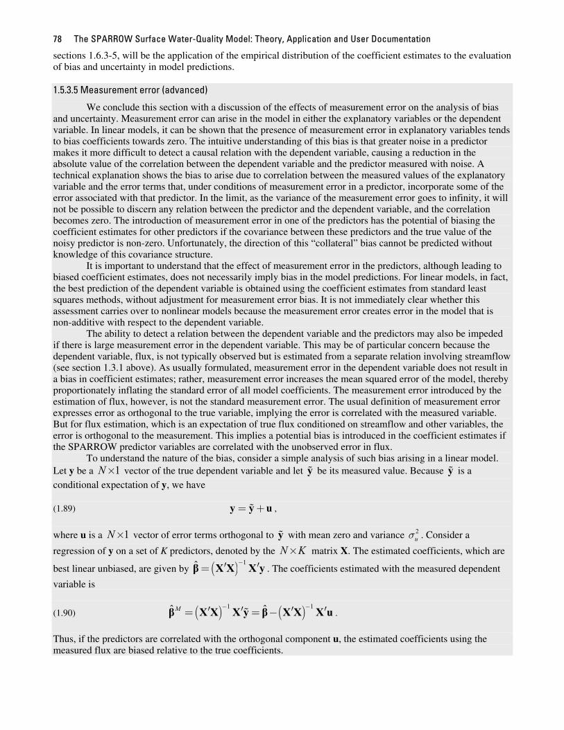
1.5.3.5 Measurement error (advanced)
We conclude this section with a discussion of the effects of measurement error on the analysis of bias and uncertainty. Measurement error can arise in the model in either the explanatory variables or the dependent variable. In linear models, it can be shown that the presence of measurement error in explanatory variables tends to bias coefficients towards zero. The intuitive understanding of this bias is that greater noise in a predictor makes it more difficult to detect a causal relation with the dependent variable, causing a reduction in the absolute value of the correlation between the dependent variable and the predictor measured with noise. A technical explanation shows the bias to arise due to correlation between the measured values of the explanatory variable and the error terms that, under conditions of measurement error in a predictor, incorporate some of the error associated with that predictor. In the limit, as the variance of the measurement error goes to infinity, it will not be possible to discern any relation between the predictor and the dependent variable, and the correlation becomes zero. The introduction of measurement error in one of the predictors has the potential of biasing the coefficient estimates for other predictors if the covariance between these predictors and the true value of the noisy predictor is non-zero. Unfortunately, the direction of this “collateral” bias cannot be predicted without knowledge of this covariance structure.
It is important to understand that the effect of measurement error in the predictors, although leading to biased coefficient estimates, does not necessarily imply bias in the model predictions. For linear models, in fact, the best prediction of the dependent variable is obtained using the coefficient estimates from standard least squares methods, without adjustment for measurement error bias. It is not immediately clear whether this assessment carries over to nonlinear models because the measurement error creates error in the model that is non-additive with respect to the dependent variable.
The ability to detect a relation between the dependent variable and the predictors may also be impeded if there is large measurement error in the dependent variable. This may be of particular concern because the dependent variable, flux, is not typically observed but is estimated from a separate relation involving streamflow (see section 1.3.1 above). As usually formulated, measurement error in the dependent variable does not result in a bias in coefficient estimates; rather, measurement error increases the mean squared error of the model, thereby proportionately inflating the standard error of all model coefficients. The measurement error introduced by the estimation of flux, however, is not the standard measurement error. The usual definition of measurement error expresses error as orthogonal to the true variable, implying the error is correlated with the measured variable. But for flux estimation, which is an expectation of true flux conditioned on streamflow and other variables, the error is orthogonal to the measurement. This implies a potential bias is introduced in the coefficient estimates if the SPARROW predictor variables are correlated with the unobserved error in flux.
To understand the nature of the bias, consider a simple analysis of such bias arising in a linear model. Let y be a vector of the true dependent variable and let be its measured value. Because is a 1N× y yconditional expectation of y, we have (1.89) , = +y y u
where u is a vector of error terms orthogonal to with mean zero and variance . Consider a 1N× y 2uσ
regression of y on a set of K predictors, denoted by the matrix X. The estimated coefficients, which are N K×
best linear unbiased, are given by ( ) 1ˆ −′=β X X X y′ . The coefficients estimated with the measured dependent
variable is
(1.90) . ( ) ( )1 1ˆ ˆM − −′ ′ ′ ′= = −β X X X y β X X X u
Thus, if the predictors are correlated with the orthogonal component u, the estimated coefficients using the measured flux are biased relative to the true coefficients.
Part 1: A Theoretical and Practical Introduction to SPARROW 79
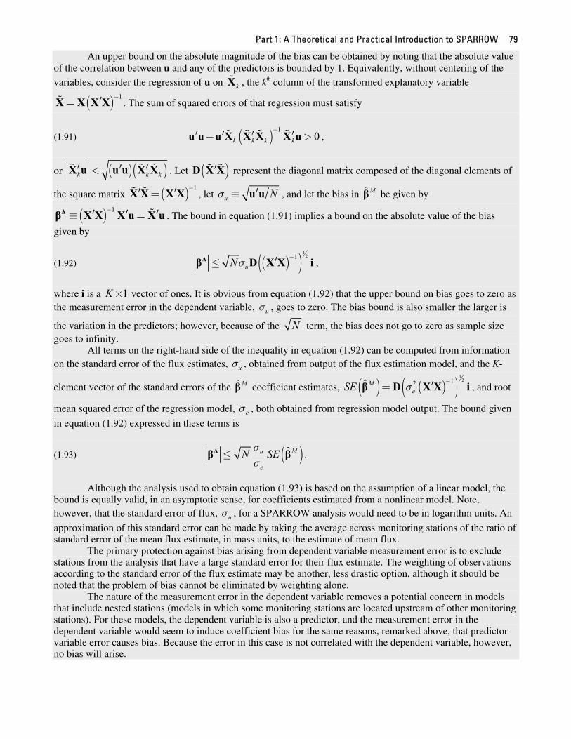
An upper bound on the absolute magnitude of the bias can be obtained by noting that the absolute value of the correlation between u and any of the predictors is bounded by 1. Equivalently, without centering of the variables, consider the regression of u on , the kkX
th column of the transformed explanatory variable
( ) 1−′=X X X X . The sum of squared errors of that regression must satisfy
(1.91) , ( ) 10k k k k
−′ ′ ′ ′− >u u u X X X X u
or ( )( )k k k′ ′ ′<X u u u X X . Let ( )′XD X represent the diagonal matrix composed of the diagonal elements of
the square matrix ( ) 1−′ ′=X X X X , let u Nσ ′≡ u u , and let the bias in ˆ Mβ be given by
( ) 1−′ ′ ′≡ =Δβ X X X u X u . The bound in equation (1.91) implies a bound on the absolute value of the bias
given by
(1.92) ( )( )1
21uNσ
−′≤Δβ D X X i ,
where i is a 1K× vector of ones. It is obvious from equation (1.92) that the upper bound on bias goes to zero as the measurement error in the dependent variable, , goes to zero. The bias bound is also smaller the larger is uσ
the variation in the predictors; however, because of the N term, the bias does not go to zero as sample size goes to infinity.
All terms on the right-hand side of the inequality in equation (1.92) can be computed from information on the standard error of the flux estimates, , obtained from output of the flux estimation model, and the K-uσ
element vector of the standard errors of the ˆ Mβ coefficient estimates, ( ) ( )( )1
212ˆMeSE σ
−′=β D X X i , and root
mean squared error of the regression model, , both obtained from regression model output. The bound given eσin equation (1.92) expressed in these terms is
(1.93) ( )ˆMu
e
N SEσσ
≤Δβ β .
Although the analysis used to obtain equation (1.93) is based on the assumption of a linear model, the bound is equally valid, in an asymptotic sense, for coefficients estimated from a nonlinear model. Note, however, that the standard error of flux, , for a SPARROW analysis would need to be in logarithm units. An uσapproximation of this standard error can be made by taking the average across monitoring stations of the ratio of standard error of the mean flux estimate, in mass units, to the estimate of mean flux.
The primary protection against bias arising from dependent variable measurement error is to exclude stations from the analysis that have a large standard error for their flux estimate. The weighting of observations according to the standard error of the flux estimate may be another, less drastic option, although it should be noted that the problem of bias cannot be eliminated by weighting alone.
The nature of the measurement error in the dependent variable removes a potential concern in models that include nested stations (models in which some monitoring stations are located upstream of other monitoring stations). For these models, the dependent variable is also a predictor, and the measurement error in the dependent variable would seem to induce coefficient bias for the same reasons, remarked above, that predictor variable error causes bias. Because the error in this case is not correlated with the dependent variable, however, no bias will arise.
The SPARROW Surface Water-Quality Model: Theory, Application and User Documentation 80
1.5.4 Evaluation of the model parameters
Parameter evaluation in SPARROW modeling has the objectives of determining whether a converged model gives statistically sound and physically interpretable coefficient values. The process of parameter evaluation commonly becomes a delicate balance, with allowances being made for one consideration in order to accommodate strong evidence or beliefs from the other. If after completing this section the reader retains a view that statistics is best practiced as an art, a proper understanding of this process will have been achieved.
1.5.4.1 Statistical evaluations
The first objective in parameter evaluation entails the appraisal of model parameters for statistical significance and the quantification of uncertainty (i.e., the range of probable values of the parameters). This provides important information for identifying unique model specifications (i.e., parameters and values for which the model predictions are sensitive) and determining the level of model complexity (i.e., number and types of explanatory variables and model functions) that can be empirically supported by the stream monitoring data. The emphasis on parameter estimation in SPARROW models has the objective of identifying the important contaminant sources and factors affecting mean-annual contaminant transport over large spatial scales in soils and in ground and surface waters.
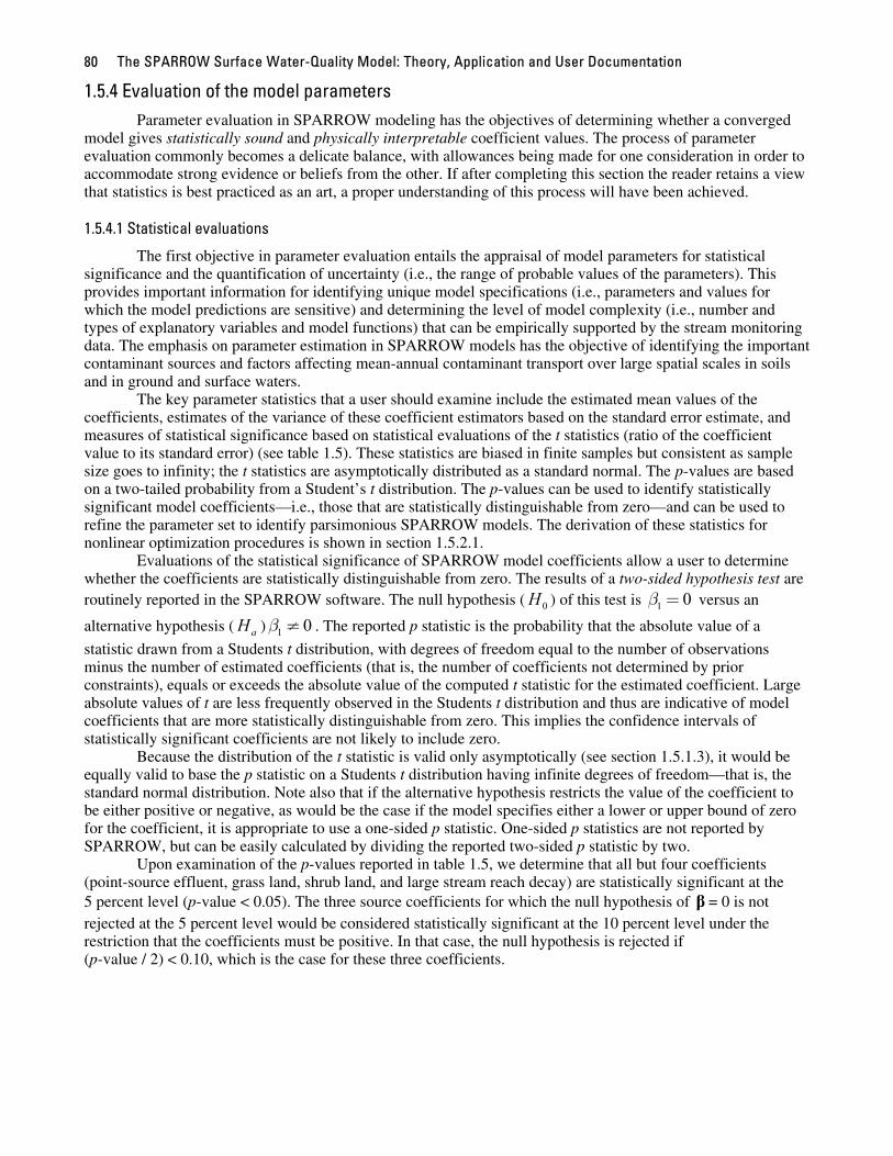
The key parameter statistics that a user should examine include the estimated mean values of the coefficients, estimates of the variance of these coefficient estimators based on the standard error estimate, and measures of statistical significance based on statistical evaluations of the t statistics (ratio of the coefficient value to its standard error) (see table 1.5). These statistics are biased in finite samples but consistent as sample size goes to infinity; the t statistics are asymptotically distributed as a standard normal. The p-values are based on a two-tailed probability from a Student’s t distribution. The p-values can be used to identify statistically significant model coefficients—i.e., those that are statistically distinguishable from zero—and can be used to refine the parameter set to identify parsimonious SPARROW models. The derivation of these statistics for nonlinear optimization procedures is shown in section 1.5.2.1.
Evaluations of the statistical significance of SPARROW model coefficients allow a user to determine whether the coefficients are statistically distinguishable from zero. The results of a two-sided hypothesis test are routinely reported in the SPARROW software. The null hypothesis ( ) of this test is versus an
alternative hypothesis ( ) . The reported p statistic is the probability that the absolute value of a
statistic drawn from a Students t distribution, with degrees of freedom equal to the number of observations minus the number of estimated coefficients (that is, the number of coefficients not determined by prior constraints), equals or exceeds the absolute value of the computed t statistic for the estimated coefficient. Large absolute values of t are less frequently observed in the Students t distribution and thus are indicative of model coefficients that are more statistically distinguishable from zero. This implies the confidence intervals of statistically significant coefficients are not likely to include zero.
0H 1 0β =
aH 1 0β ≠
Because the distribution of the t statistic is valid only asymptotically (see section 1.5.1.3), it would be equally valid to base the p statistic on a Students t distribution having infinite degrees of freedom—that is, the standard normal distribution. Note also that if the alternative hypothesis restricts the value of the coefficient to be either positive or negative, as would be the case if the model specifies either a lower or upper bound of zero for the coefficient, it is appropriate to use a one-sided p statistic. One-sided p statistics are not reported by SPARROW, but can be easily calculated by dividing the reported two-sided p statistic by two.
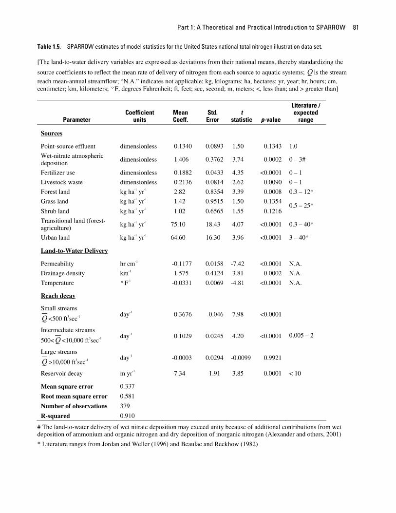
Upon examination of the p-values reported in table 1.5, we determine that all but four coefficients (point-source effluent, grass land, shrub land, and large stream reach decay) are statistically significant at the 5 percent level (p-value < 0.05). The three source coefficients for which the null hypothesis of = 0 is not rejected at the 5 percent level would be considered statistically significant at the 10 percent level under the restriction that the coefficients must be positive. In that case, the null hypothesis is rejected if (p-value / 2) < 0.10, which is the case for these three coefficients.
β
Part 1: A Theoretical and Practical Introduction to SPARROW 81
Table 1.5. SPARROW estimates of model statistics for the United States national total nitrogen illustration data set.
[The land-to-water delivery variables are expressed as deviations from their national means, thereby standardizing the
source coefficients to reflect the mean rate of delivery of nitrogen from each source to aquatic systems; Q is the stream reach mean-annual streamflow; “N.A.” indicates not applicable; kg, kilograms; ha, hectares; yr, year; hr, hours; cm, centimeter; km, kilometers; ° F, degrees Fahrenheit; ft, feet; sec, second; m, meters; <, less than; and > greater than]
Parameter Coefficient
units Mean Coeff.
Std. Error
t statistic p-value
Literature / expected
range
Sources
Point-source effluent dimensionless 0.1340 0.0893 1.50 0.1343 1.0
Wet-nitrate atmospheric deposition dimensionless 1.406 0.3762 3.74 0.0002 0 – 3#
Fertilizer use dimensionless 0.1882 0.0433 4.35 <0.0001 0 – 1
Livestock waste dimensionless 0.2136 0.0814 2.62 0.0090 0 – 1
Forest land kg ha-1 yr-1 2.82 0.8354 3.39 0.0008 0.3 – 12*
Grass land kg ha-1 yr-1 1.42 0.9515 1.50 0.1354
Shrub land kg ha-1 yr-1 1.02 0.6565 1.55 0.1216 0.5 – 25*
Transitional land (forest-agriculture) kg ha-1 yr-1 75.10 18.43 4.07 <0.0001 0.3 – 40*
Urban land kg ha-1 yr-1 64.60 16.30 3.96 <0.0001 3 – 40*
Land-to-Water Delivery
Permeability hr cm-1 -0.1177 0.0158 -7.42 <0.0001 N.A.
Drainage density km-1 1.575 0.4124 3.81 0.0002 N.A.
Temperature ° F-1 -0.0331 0.0069 -4.81 <0.0001 N.A.
Reach decay
Small streams
Q <500 ft3sec-1 day-1 0.3676 0.046 7.98 <0.0001
Intermediate streams
500<Q <10,000 ft3sec-1 day-1 0.1029 0.0245 4.20 <0.0001
Large streams
Q >10,000 ft3sec-1 day-1 -0.0003 0.0294 -0.0099 0.9921
0.005 – 2
Reservoir decay m yr-1 7.34 1.91 3.85 0.0001 < 10
Mean square error 0.337
Root mean square error 0.581
Number of observations 379
R-squared 0.910
# The land-to-water delivery of wet nitrate deposition may exceed unity because of additional contributions from wet deposition of ammonium and organic nitrogen and dry deposition of inorganic nitrogen (Alexander and others, 2001)
* Literature ranges from Jordan and Weller (1996) and Beaulac and Reckhow (1982)
The SPARROW Surface Water-Quality Model: Theory, Application and User Documentation 82
The two-sided t statistic reported in SPARROW is equivalent to a partial F test (i.e., ) in which the test evaluates the statistical significance of a complex model that results from the addition of one additional explanatory variable to a simple model that has all of the other variables present. The simple model is therefore nested within the more complex model and differs by only one explanatory variable. By contrast, cases may exist in which a nested F test needs to be applied to determine whether the addition of more than one explanatory variable (e.g., the collection of aquatic decay variables or land-to-water delivery variables) results in a significant improvement in the performance of the model (i.e., improved explanation of the variability in the response variable). This test is not calculated as part of the SPARROW software, but can be manually calculated by the user. The nested F statistic is expressed as
2F t=
(1.94)
( )( )
S C
S C
C
C
SSE SSEdf dfF SSEdf
−−
= ,
where SSES is the sum of squares of error of the simple model with degrees of freedom, dfS; and SSEC is the sum of squares of error of the complex model with degrees of freedom, dfC (degrees of freedom equal the difference between the number of observations and the number of estimated parameters—excluding parameters determined by a prior constraint). The test provides a measure of the tradeoff between the reduction in error (i.e., improved explanatory power) that results from a more complex model and the estimation penalty that results from the addition of parameters and the corresponding reduction in the model degrees of freedom. The test, therefore, assesses whether the reduction in error is statistically worth the loss of information for estimating the model as measured by the degrees of freedom. As with the t test, the F test is valid only asymptotically, implying it could be replaced by a chi-square test with degrees of freedom equal to dfs – dfc.
One example use of a nested F test in SPARROW is the evaluation of a hypothesis concerning whether the addition of aquatic decay parameters to a model collectively results in a statistically significant improvement in the overall model performance. In this test, we compare the more complex model containing aquatic decay variables as given in table 1.5 (MSE equals 0.337) with a simple model wherein both the in-stream and reservoir decay coefficients are removed (MSE equals 0.767). In this case, an F statistic is computed such that
(1.95)
(283.6 122.4)(379 12) (379 16) 119.5122.4
(379 16)
F
−− − −= =
−
.
The p-value (less than 0.00001) associated with this F statistic is highly significant, and indicates that the addition of the aquatic decay coefficients provides a significant improvement in the explanatory power of the model. Note that this test does not indicate that all of the aquatic coefficients are significantly distinguishable from zero, but only that at least one of the coefficients is. The results of a partial F test (i.e., the individual coefficient t statistics) must be examined to determine the significance of individual coefficients.
1.5.4.2 Physical interpretations
A second complementary objective in assessing SPARROW model parameters is the evaluation of the parameters for their physical interpretability. This objective entails the evaluation of the sign and magnitude of model coefficients to test hypotheses about the importance of different contaminant sources and the hydrologic and biogeochemical processes that are represented by the explanatory variables of the model. The interpretability of the parameters and their relation to specific processes is enhanced in SPARROW by the use of a mass balance, mechanistic structure that explicitly separates the terrestrial and aquatic properties of watersheds and accounts for nonlinear interactions among watershed properties (see section 1.2.2), together with an emphasis on the statistical estimation of parameter values. As discussed in section 1.2.3, the SPARROW model
Part 1: A Theoretical and Practical Introduction to SPARROW 83
parameters reflect the net effects over large spatial scales of an aggregate set of hydrologic and biogeochemical processes and human-related activities.
The sign of SPARROW model coefficients can be evaluated to determine the direction of the relation of any explanatory variable to the in-stream estimates of the mean-annual flux (i.e., the model response variable). The direction of the relation should be assessed for consistency with the anticipated response based on available theoretical or empirical information about processes that may be related to individual explanatory factors. For example, for the model results shown in table 1.5, a negative sign on the soil permeability coefficient indicates that total nitrogen loads in streams are inversely related to permeability—i.e., in-stream loads of nitrogen are generally lower in watersheds with highly permeable soils. This relation is frequently found in SPARROW nitrogen models and is consistent with the storage or permanent removal (i.e., denitrification) of nitrogen in soils and the subsurface. The relation indicates that nitrogen losses are larger (and in-stream nitrogen flux smaller) in watersheds where water and nitrogen are more readily routed through permeable soils. The sign of the coefficient is also important in estimating physically meaningful contaminant source terms in SPARROW. Interpretable sources within the model are generally expected to contribute positive mass to the watersheds. In fact, we often constrain the sources to be positive; thus, a one-sided hypothesis test is frequently of interest in evaluating the statistical evidence of the importance of source inputs in the model. Constraints on the coefficient sign are generally not applied to land-to-water delivery factors as there is commonly no compelling prior expectation as to the nature of the physical relation to flux. Constraints on the aquatic decay factors are also generally unnecessary; however, there may be a need to constrain the “large” river decay rates (mean rates are frequently near zero with a considerable fraction of the parameter distribution below zero) and reservoir decay rates to positive values in bootstrap executions of final SPARROW models to obtain a more physically realistic simulation of contaminant transport in rivers (i.e., negative portions of the parameter distribution may unrealistically skew the estimates of the mean; e.g., see discussion in Alexander, Elliott, and others, 2002).
The values of selected source and aquatic decay coefficients should also be evaluated to determine whether they are consistent with the range of values expected on the basis of literature studies and the prevailing information on experimental reaction rates. For the source coefficients to be easily interpreted, they must be standardized for mean levels of the land-to-water delivery variables (see section 1.4.3), such as those shown in table 1.5. It is important to note that the coefficients of the land-to-water factors cannot be interpreted individually in terms of a contaminant transport rate that is specific to the landscape property, but must be combined with individual sources to quantify an aggregate delivery of the contaminant mass to streams. By contrast, the aquatic decay coefficients can be directly interpreted without any standardization. For example, the rates of nitrogen removal in streams (ranging from near zero to 0.37 day-1) and reservoirs (7.3 meters yr-1) reported in table 1.5 can be directly compared to literature rates, as illustrated in previous sections of this report.
Source-related coefficients that are based on source inputs expressed in areal units, such as the land-use source terms (forest, grass, shrub, urban) in table 1.5, describe the mass per unit area delivered to streams from these land areas. These areal expressions of contaminant transport or “export” can be directly compared with ranges of export coefficients that are frequently reported in the literature (e.g., Beaulac and Reckhow, 1982). Coefficients reported for different land uses such as those in table 1.5 generally compare favorably with export coefficients reported in the literature. The SPARROW estimated export coefficients in table 1.5 are standardized to reflect the supply and delivery of nitrogen to aquatic systems under the mean levels of the landscape delivery factors in the model. Of course, one complicating aspect of such a comparison is that the literature export coefficients implicitly include the effects of watershed properties (e.g., soils, climate, in-stream processes) on nutrient transport that likely differ from those in the SPARROW model. Nevertheless, SPARROW estimates and export coefficients reported in the literature are consistent in indicating that the nutrient supply and delivery to streams and reservoirs is generally larger in urban and agricultural watersheds; much lower export coefficients are found in forests and in grass and shrub lands, where relatively small natural sources (e.g., nitrogen fixation by vegetation) of nitrogen predominate.
Other source coefficients that are expressed in dimensionless units provide a measure of the fraction of the contaminant that is delivered from each source to streams, rivers, and reservoirs. These coefficients can be evaluated to determine how reasonably they reflect the net mean rates of contaminant removal by a source as part of the delivery to aquatic systems. For example, about 18 percent of the fertilizer inputs of nitrogen are delivered to streams based on the model results reported in table 1.5. Such large losses of fertilizer inputs are generally expected and reflect the numerous processes and activities that remove nitrogen from agricultural lands and along subsurface flow paths. The estimated fertilizer coefficient reflects the aggregate effects of these
The SPARROW Surface Water-Quality Model: Theory, Application and User Documentation 84
factors and may include the volatilization of ammonia fertilizer forms, the removal of nitrogen in harvested crops, and long-term immobilization of nitrogen and denitrification in soils and ground waters. In the case of atmospheric deposition, the greater than unity coefficient of 1.4 is consistent with additional contributions from wet deposition of organic nitrogen and dry deposition of inorganic nitrogen, which are not included in the wet nitrate measurements input to the model. This result would be expected, provided that these unmeasured quantities are correlated with the measured wet deposition, which is commonly the case (Alexander and others, 2001).
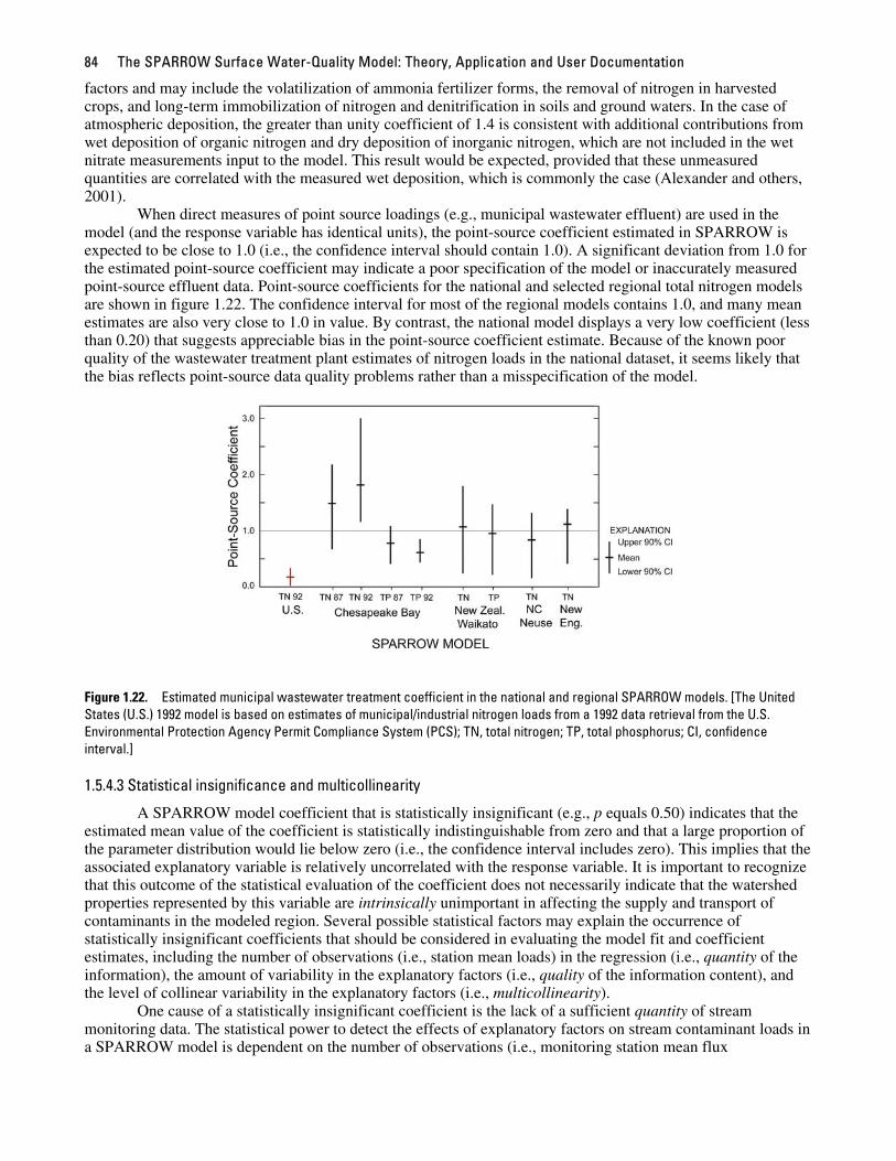
When direct measures of point source loadings (e.g., municipal wastewater effluent) are used in the model (and the response variable has identical units), the point-source coefficient estimated in SPARROW is expected to be close to 1.0 (i.e., the confidence interval should contain 1.0). A significant deviation from 1.0 for the estimated point-source coefficient may indicate a poor specification of the model or inaccurately measured point-source effluent data. Point-source coefficients for the national and selected regional total nitrogen models are shown in figure 1.22. The confidence interval for most of the regional models contains 1.0, and many mean estimates are also very close to 1.0 in value. By contrast, the national model displays a very low coefficient (less than 0.20) that suggests appreciable bias in the point-source coefficient estimate. Because of the known poor quality of the wastewater treatment plant estimates of nitrogen loads in the national dataset, it seems likely that the bias reflects point-source data quality problems rather than a misspecification of the model.
Figure 1.22. Estimated municipal wastewater treatment coefficient in the national and regional SPARROW models. [The United States (U.S.) 1992 model is based on estimates of municipal/industrial nitrogen loads from a 1992 data retrieval from the U.S. Environmental Protection Agency Permit Compliance System (PCS); TN, total nitrogen; TP, total phosphorus; CI, confidence interval.]
1.5.4.3 Statistical insignificance and multicollinearity
A SPARROW model coefficient that is statistically insignificant (e.g., p equals 0.50) indicates that the estimated mean value of the coefficient is statistically indistinguishable from zero and that a large proportion of the parameter distribution would lie below zero (i.e., the confidence interval includes zero). This implies that the associated explanatory variable is relatively uncorrelated with the response variable. It is important to recognize that this outcome of the statistical evaluation of the coefficient does not necessarily indicate that the watershed properties represented by this variable are intrinsically unimportant in affecting the supply and transport of contaminants in the modeled region. Several possible statistical factors may explain the occurrence of statistically insignificant coefficients that should be considered in evaluating the model fit and coefficient estimates, including the number of observations (i.e., station mean loads) in the regression (i.e., quantity of the information), the amount of variability in the explanatory factors (i.e., quality of the information content), and the level of collinear variability in the explanatory factors (i.e., multicollinearity).
One cause of a statistically insignificant coefficient is the lack of a sufficient quantity of stream monitoring data. The statistical power to detect the effects of explanatory factors on stream contaminant loads in a SPARROW model is dependent on the number of observations (i.e., monitoring station mean flux
Part 1: A Theoretical and Practical Introduction to SPARROW 85
measurements) used in the nonlinear regression. As discussed in section 1.2.4, the number of stream monitoring stations influences the level of complexity (i.e., number of explanatory variables) that can be supported in SPARROW models. For example, we find that fewer explanatory variables—typically from six to eight—are statistically significant in many of the regional models as compared to upwards of 18 or more variables in the national model. Therefore, models with fewer station flux measurements are generally more limited in their ability to identify statistically significant explanatory variables.
A second cause of a statistically insignificant coefficient is the lack of sufficient spatial variability in an explanatory factor (in the introduction, we cited this as related to issues of the quality of the data). The effect of explanatory factors on stream contaminant flux can be difficult to detect in SPARROW models if the spatial variability in the factor is relatively small over the modeled region. For example, precipitation is clearly an important contributor in determining the magnitude of stream contaminant flux at regional and national spatial scales. In many of the regional SPARROW models, however, variability in mean-annual precipitation is small across the regions (i.e., variations that are less than an order of magnitude) and this factor is rarely found to be statistically significant as a land-to-water delivery factor. By contrast, mean-annual precipitation varies by several orders of magnitude in the national SPARROW model and in the New Zealand national model (Elliott and others, 2005) and has been found to be highly significant as a delivery factor in recent versions of these models. Given the level of statistical power for many of the regional models, the spatial variability in the regional measures of precipitation in comparison to that of other controlling factors in the models is typically insufficient to support the estimation of an explicit precipitation term in the models. It is important to note that this does not imply that a model without precipitation data as input is invalid as a prediction tool. Indeed, such a model can be reliably used to predict in-stream flux and the contributions of pollutant sources to streams. The model does not, however, provide an explicit description of how precipitation influences pollutant flux, and therefore could not be used to assess climate-related effects on stream water quality.
It is also noteworthy that the source coefficient for a relatively small contaminant source (e.g., natural or background inputs of nitrogen) may be difficult to estimate with a high degree of statistical significance because the true numerical value of the coefficient is small, especially relative to its level of precision (i.e., standard error of estimate). The detection of only weak statistical significance for such a variable does not necessarily provide sufficient cause to exclude it, especially if the intent in using the model is to provide a comprehensive understanding of contaminant sources. For example, the grass and shrub land export coefficients are only weakly significant in the national SPARROW model illustrated in table 1.5, although the level of precision of these terms is equal to or even surpasses the precision associated with the more highly significant forest export coefficient. Nitrogen from natural fixation on grass and shrub lands is generally smaller in comparison to nitrogen generated from fixation and other sources in forests (Jordan and Weller, 1996; nitrogen export from forested land may also include some contributions from atmospheric deposition). This is a likely explanation for why the estimated mean nitrogen export from grass and shrub land (table 1.5) is only about one half of that estimated for forested lands.
Finally, another potential explanation for the lack of statistical significance in two or more explanatory variables is the effect of multicollinearity on the variance of the model parameters. Multicollinearity describes the presence of high levels of correlation between two or more explanatory variables in a regression model that cause all of the correlated variables to have statistically insignificant coefficients. SPARROW provides several statistics and matrices that are useful for evaluating the presence and causes of multicollinearity.
The problem of mulicollinearity is one of model interpretability rather than model validity. The presence of multicollinearity does not imply the model coefficients or their standard errors are estimated with bias. Moreover, the predictions from the model are asymptotically minimum variance unbiased. The most serious consequence of multicollinearity is that coefficients associated with collinear variables (or, in the case of the nonlinear SPARROW model, collinear gradients) are imprecisely estimated. This lack of precision is reflected in large standard errors and a tendency for coefficients of collinear variables to be individually insignificant. Thus, in cases of multicollinearity, a coefficient estimated as statistically insignificant may in fact represent an important process in the model, but its incremental contribution to model fit is masked by other collinear processes. Indicators of multicollinearity are useful therefore in distinguishing coefficients that have potential significance and coefficients that truly should be dropped from the model.
An interesting situation arises if two coefficients are collinear but one coefficient is statistically significant and the other is not. It can be shown that collinearity does not affect the ratio of variance between two coefficients or, therefore, the ratio of t-statistics. It can be concluded therefore that the signal being
The SPARROW Surface Water-Quality Model: Theory, Application and User Documentation 86
transmitted through the significant coefficient from its associated predictor is quantitatively more important than the signal transmitted through the insignificant coefficient. In other words, collinearity in this case is not so strong that it masks the contribution of a quantitatively important predictor. For example, as illustration of this, we modified the total nitrogen model described in section 1.4.4 so two highly spatially correlated atmospheric deposition sources, wet nitrate and ammonia, are included in the model. In the resulting model, we find that only the nitrate deposition coefficient is statistically significant (p equals 0.0007), whereas the ammonia deposition coefficient is negative and statistically insignificant (p equals 0.90). This result suggests that the strongest atmospheric deposition effect on in-stream nitrogen flux is apparent from the wet nitrate deposition source in the model.
The variance inflation factor (VIF) is a commonly used statistic for determining the importance of multicollinearity. Under linear least squares, the variance inflation factor for coefficient k, VIFk, is given by the
kth diagonal element of the ( ) 1−′X X matrix, where is the N ×(K – 1) matrix of predictor variables, excluding
the intercept, centered and scaled to unit length (Montgomery and Peck, 1982). That is, observation i for
predictor variable k has been transformed according to
X
( ) 1 2ik k kX ikX X S= − , where kX is the mean of the N
observations of the kth variable and ( 2
1
N
k iki
S X X=
= −∑ )k . It can be shown (Montgomery and Peck, 1982) that
(1.96) 2
11k
k
VIFR
=−
,
where 2kR is the coefficient of multiple determination from the regression of Xk on the remaining K – 1
predictor variables, including an intercept. If there is a close relation between variable k and the remaining variables, then 2
kR is near one and the variance inflation factor is large. Conversely, if the kth variable is
independent of the other variables, then 2kR is near zero and the variance inflation factor is near its lower bound
of one. Another useful interpretation of the variance inflation factor relates to the effect that collinearity of the
predictors has on coefficient variance, t-statistics, and confidence intervals (Montgomery and Peck, 1982). The square root of the kth coefficient’s variance, given by the model root mean squared error times the kth diagonal element of the inverse of the matrix, is proportional to the length of the k′X X th coefficient’s symmetric confidence interval and is inversely proportional to the magnitude of the kth coefficient’s t-statistic. Suppose observations could be chosen in such a way that each predictor is independent of all others but retains the predictor variances exhibited in the original sample. Such a sampling scheme, called an orthogonal design, has no collinearity and results in the smallest possible coefficient variances—that is, the smallest possible values along the diagonal of the matrix. Consequently, orthogonal design sampling results in the smallest possible (symmetric) confidence intervals and largest possible t-statistics for the estimated coefficients. It can be shown that the variance inflation factor for a coefficient is equal to the ratio of that coefficient’s variance to the coefficient’s variance that would be possible under orthogonal design. The square root of the variance inflation factor, therefore, represents the proportion by which the t-statistic could be increased if multicollinearity were eliminated. This insight provides a useful interpretation of the variance inflation factor. If a coefficient is insignificant, and inflating the coefficient’s t-statistic by the square root of its variance inflation factor fails to make the coefficient significant, then multicollinearity is an unlikely explanation of the coefficient’s insignificance. Conversely, if applying the inflation factor makes the coefficient significant then it is possible that multicollinearity is masking the significance of the coefficient.
′X X
To apply the variance inflation factor to a nonlinear model, and thus provide for interpretation of collinear coefficients as described above, the gradients (see section 1.5.1.2) evaluated at the final coefficient
estimates, , are substituted for the predictor variables, X. Because a SPARROW model typically has no
intercept, however, it is inappropriate to center the gradients prior to normalizing to unit length. This is because the R
( )* ˆβf β
2 statistic implied by a variance inflation factor computed from centered predictors is a valid indicator of
Part 1: A Theoretical and Practical Introduction to SPARROW 87
explanatory power only if the set of predictors includes an intercept; the relation between the variance inflation factor computed using centered predictors and coefficient variance does not hold absent the intercept term. SPARROW automatically tests the gradient vectors to determine if they include an intercept term. If no intercept is present, the normalization of the gradient vectors is performed without centering, resulting in the
computation of an uncentered variance inflation factor, VIF . This factor can be used to determine the potential effect collinearity has on the coefficient t-statistics in exactly the same way the standard variance inflation factor is used if an intercept is present.
The uncentered variance inflation factor also bears a relation to a fit statistic. That is,
( )2VIF 1 1k kR= − , where 2kR is the uncentered r-square statistic formed by regressing the kth gradient on the
remaining K – 1 gradients. The uncentered r-square statistic, defined as the ratio of the sum of squares of the regression predicted values to the sum of squares of the regression dependent variable, is commonly used in place of the normal r-square if the regression does not include an intercept. The uncentered r-square statistic is bounded between 0 and 1 and will always exceed the standard r-square. This implies that the uncentered variance inflation factor always exceeds the standard variance inflation factor, the relation between them being
(1.97) 2
1VIF VIF 1CV
k kk
⎛ ⎞⎟⎜ ⎟= +⎜ ⎟⎜ ⎟⎜⎝ ⎠,
where CV is the coefficient of variation for the kkth gradient.
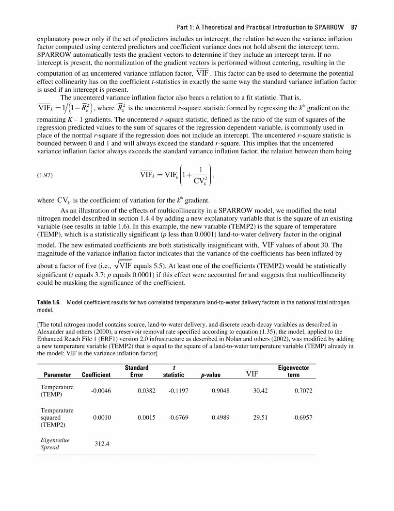
As an illustration of the effects of multicollinearity in a SPARROW model, we modified the total nitrogen model described in section 1.4.4 by adding a new explanatory variable that is the square of an existing variable (see results in table 1.6). In this example, the new variable (TEMP2) is the square of temperature (TEMP), which is a statistically significant (p less than 0.0001) land-to-water delivery factor in the original
model. The new estimated coefficients are both statistically insignificant with, VIF values of about 30. The magnitude of the variance inflation factor indicates that the variance of the coefficients has been inflated by
about a factor of five (i.e., VIF equals 5.5). At least one of the coefficients (TEMP2) would be statistically significant (t equals 3.7; p equals 0.0001) if this effect were accounted for and suggests that multicollinearity could be masking the significance of the coefficient.
Table 1.6. Model coefficient results for two correlated temperature land-to-water delivery factors in the national total nitrogen model. [The total nitrogen model contains source, land-to-water delivery, and discrete reach-decay variables as described in Alexander and others (2000), a reservoir removal rate specified according to equation (1.35); the model, applied to the Enhanced Reach File 1 (ERF1) version 2.0 infrastructure as described in Nolan and others (2002), was modified by adding a new temperature variable (TEMP2) that is equal to the square of a land-to-water temperature variable (TEMP) already in the model; VIF is the variance inflation factor]
Parameter Coefficient Standard
Error t
statistic p-value VIF Eigenvector
term
Temperature (TEMP) -0.0046 0.0382 -0.1197 0.9048 30.42 0.7072
Temperature squared (TEMP2)
-0.0010 0.0015 -0.6769 0.4989 29.51 -0.6957
Eigenvalue Spread 312.4
The SPARROW Surface Water-Quality Model: Theory, Application and User Documentation 88
Another statistic reported by SPARROW to help identify multicollinearity is the eigenvalue spread. The
eigenvalue spread is computed from the eigenvalues of the matrix of normalized gradients. If an intercept is absent from the model then the normalized gradients are uncentered prior to normalization. The eigenvalues
of the K ×K matrix represent the K roots, denoted λ , of the equation . Because
is a positive semi-definite matrix, all of its eigenvalues must be greater than or equal to zero. The eigenvalue spread is defined as
′X X
′X X ( )det 0λ′ − =X X I
′X X
(1.98) max
min
λκ
λ= .
If the matrix is nearly singular, an implication of multicollinearity among the gradients, then one or more eigenvalues will be near zero; a large value for eigenvalue spread is therefore evidence of multicollinearity. In practice, if the eigenvalue spread is less than 100 there is no serious problem with multicollinearity (Montgomery and Peck, 1982). As discussed above, however, issues of collinearity make sense only in the context of determining coefficient significance. The fact that a general model statistic like the eigenvalue spread is large does not necessarily imply any of the coefficients are insignificant or help identify which coefficients have statistical significance that is sensitive to collinearity. According to our illustration model results in table 1.6, the eigenvalue spread was reported as being well above 100.
′X X
Perhaps the most useful interpretation derived from the matrix is the use of its eigensystem for determining which coefficients are related to each other through collinear gradients. Inference on this issue can
be ascertained by looking at the eigenvectors corresponding to very small eigenvalues. The matrix can be factored into the following eigensystem
′X X
′X X
(1.99) , ′ ′=X X CΛC
where is a diagonal matrix whose elements are the eigenvalues, λ , of , and C is a K ×K orthogonal matrix having the property that . The k
Λ ′X X′ =C C I th column of C is called the kth eigenvector corresponding to
eigenvalue . Pre- and post-multiplying by and C results in the relation C X . Define
. Then, for each k,
kλ ′X X ′C ′ ′ =XC Λ
i
≡Z XC
(1.100) 2,
1
N
k ki
Zλ=
=∑ .
Suppose the kth eigenvalue is nearly zero—indicating collinearity. Then equation (1.100) implies that for each observation i, ,k iZ is nearly zero which, through the definition of Z, implies
(1.101) . , ,1
0K
j k i jj
C X=
≈∑
That is, the kth eigenvector represents the coefficients that define a collinear grouping of the normalized gradients. Because the normalized gradients are unitless, so too are the elements of the eigenvector, implying the values of individual terms are comparable. Therefore, the largest absolute value elements of the kth eigenvector effectively define the group of gradients that are collinear.
A table of eigenvalues and eigenvectors is reported in the SPARROW software output that lists the
eigensystem of the matrix (see figure 1.23). The first row of the eigensystem output gives the K eigenvalues, and the column beneath each eigenvalue represents the associated eigenvector. Insight into the collinear structure of the model is obtained by first looking across the first row to determine if there are any eigenvalues near zero. If an element in the first row is near zero, then the largest absolute value elements in the column below it correspond to the predictors that form a set of collinear gradients. According to our illustration results for the model given in table 1.6, the largest absolute value eigenvector elements in the column corresponding to the smallest eigenvalue appear for the two temperature variables and have values of 0.7072
′X X
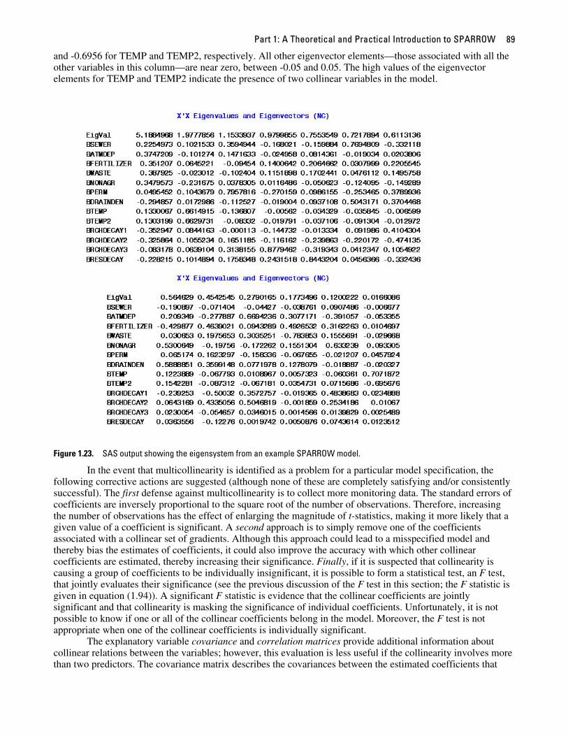
Part 1: A Theoretical and Practical Introduction to SPARROW 89
and -0.6956 for TEMP and TEMP2, respectively. All other eigenvector elements—those associated with all the other variables in this column—are near zero, between -0.05 and 0.05. The high values of the eigenvector elements for TEMP and TEMP2 indicate the presence of two collinear variables in the model.
Figure 1.23. SAS output showing the eigensystem from an example SPARROW model.
In the event that multicollinearity is identified as a problem for a particular model specification, the following corrective actions are suggested (although none of these are completely satisfying and/or consistently successful). The first defense against multicollinearity is to collect more monitoring data. The standard errors of coefficients are inversely proportional to the square root of the number of observations. Therefore, increasing the number of observations has the effect of enlarging the magnitude of t-statistics, making it more likely that a given value of a coefficient is significant. A second approach is to simply remove one of the coefficients associated with a collinear set of gradients. Although this approach could lead to a misspecified model and thereby bias the estimates of coefficients, it could also improve the accuracy with which other collinear coefficients are estimated, thereby increasing their significance. Finally, if it is suspected that collinearity is causing a group of coefficients to be individually insignificant, it is possible to form a statistical test, an F test, that jointly evaluates their significance (see the previous discussion of the F test in this section; the F statistic is given in equation (1.94)). A significant F statistic is evidence that the collinear coefficients are jointly significant and that collinearity is masking the significance of individual coefficients. Unfortunately, it is not possible to know if one or all of the collinear coefficients belong in the model. Moreover, the F test is not appropriate when one of the collinear coefficients is individually significant.
The explanatory variable covariance and correlation matrices provide additional information about collinear relations between the variables; however, this evaluation is less useful if the collinearity involves more than two predictors. The covariance matrix describes the covariances between the estimated coefficients that
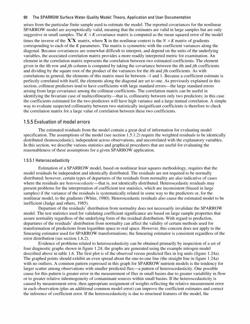
The SPARROW Surface Water-Quality Model: Theory, Application and User Documentation 90
arises from the particular finite sample used to estimate the model. The reported covariances for the nonlinear SPARROW model are asymptotically valid, meaning that the estimates are valid in large samples but are only suggestive in small samples. The K ×K covariance matrix is computed as the mean squared error of the model times the inverse of the matrix, where X in the nonlinear context is the N ×K matrix of gradients corresponding to each of the K parameters. The matrix is symmetric with the coefficient variances along the diagonal. Because covariances are somewhat difficult to interpret, and depend on the units of the underlying variables, the associated correlation matrix provides a more readily interpreted metric for examination. An element in the correlation matrix represents the correlation between two estimated coefficients. The element given in the ith row and jth column is computed by taking the covariance between the ith and jth coefficients and dividing by the square root of the product of the variances for the ith and jth coefficients. As with correlations in general, the elements of this matrix must lie between –1 and 1. Because a coefficient estimate is perfectly correlated with itself, the elements along the diagonal are set to one. As previously explained in this section, collinear predictors tend to have coefficients with large standard errors—the large standard errors arising from large covariance among the collinear coefficients. The correlation matrix can be useful in identifying the bivariate case of multicollinearity—that is, collinearity between only two predictors; in this case the coefficients estimated for the two predictors will have high variance and a large mutual correlation. A simple way to evaluate suspected collinearity between two statistically insignificant coefficients is therefore to check the correlation matrix for a large value of correlation between these two coefficients.
′X X
1.5.5 Evaluation of model errors
The estimated residuals from the model contain a great deal of information for evaluating model specification. The assumptions of the model (see section 1.5.1.2) require the weighted residuals to be identically distributed (homoscedastic), independent across observations, and uncorrelated with the explanatory variables. In this section, we describe various statistics and graphical procedures that are useful for evaluating the reasonableness of these assumptions for a given SPARROW application.
1.5.5.1 Heteroscedasticity
Estimation of a SPARROW model, based on nonlinear least squares methodology, requires that the model residuals be independent and identically distributed. The residuals are not required to be normally distributed; however, certain types of departures of the residuals from normality are also indicative of cases where the residuals are heteroscedastic—that is, not identically distributed. Heteroscedastic residuals may present problems for the interpretation of coefficient test statistics, which are inconsistent (biased in large samples) if the variance of the residuals is systematically related in some way to the predictors or, for the nonlinear model, to the gradients (White, 1980). Heteroscedastic residuals also cause the estimated model to be inefficient (Judge and others, 1985).
Departure of the residuals’ distribution from normality does not necessarily invalidate the SPARROW model. The test statistics used for validating coefficient significance are based on large sample properties that assure normality regardless of the underlying form of the residual distribution. With regard to prediction, departures of the residuals’ distribution from normality can affect the validity of certain methods used for transformation of predictions from logarithm space to real space. However, this concern does not apply to the Smearing estimator used for SPARROW transformations; the Smearing estimator is consistent regardless of the error distribution (see section 1.6.2).
Evidence of problems related to heteroscedasticity can be obtained primarily by inspection of a set of four diagnostic graphs shown in figure 1.24; the graphs are generated using the example nitrogen model described above in table 1.6. The first plot is of the observed versus predicted flux in log units (figure 1.24a). The graphed points should exhibit an even spread about the one-to-one line (the straight line in figure 1.24a) with no outliers. A common pattern expressed in this graph for SPARROW nutrient models is the tendency for larger scatter among observations with smaller predicted flux—a pattern of heteroscedasticity. One possible cause for this pattern is greater error in the measurement of flux in small basins due to greater variability in flow or to greater relative inhomogeneity of contaminant sources within small basins. If the heteroscedasticity is caused by measurement error, then appropriate assignment of weights reflecting the relative measurement error in each observation (plus an additional common model error) can improve the coefficient estimates and correct the inference of coefficient error. If the heteroscedasticity is due to structural features of the model, the
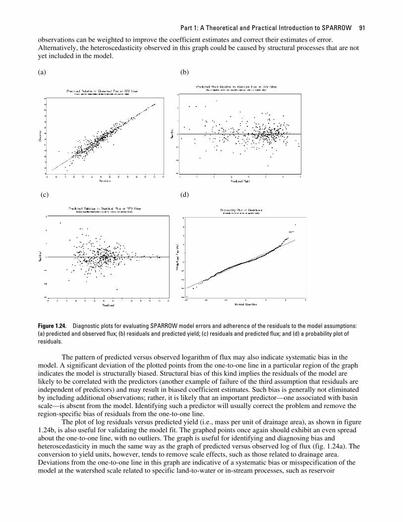
Part 1: A Theoretical and Practical Introduction to SPARROW 91
observations can be weighted to improve the coefficient estimates and correct their estimates of error. Alternatively, the heteroscedasticity observed in this graph could be caused by structural processes that are not yet included in the model.
(a) (b)
(c) (d)
Figure 1.24. Diagnostic plots for evaluating SPARROW model errors and adherence of the residuals to the model assumptions: (a) predicted and observed flux; (b) residuals and predicted yield; (c) residuals and predicted flux; and (d) a probability plot of residuals.
The pattern of predicted versus observed logarithm of flux may also indicate systematic bias in the model. A significant deviation of the plotted points from the one-to-one line in a particular region of the graph indicates the model is structurally biased. Structural bias of this kind implies the residuals of the model are likely to be correlated with the predictors (another example of failure of the third assumption that residuals are independent of predictors) and may result in biased coefficient estimates. Such bias is generally not eliminated by including additional observations; rather, it is likely that an important predictor—one associated with basin scale—is absent from the model. Identifying such a predictor will usually correct the problem and remove the region-specific bias of residuals from the one-to-one line.
The plot of log residuals versus predicted yield (i.e., mass per unit of drainage area), as shown in figure 1.24b, is also useful for validating the model fit. The graphed points once again should exhibit an even spread about the one-to-one line, with no outliers. The graph is useful for identifying and diagnosing bias and heteroscedasticity in much the same way as the graph of predicted versus observed log of flux (fig. 1.24a). The conversion to yield units, however, tends to remove scale effects, such as those related to drainage area. Deviations from the one-to-one line in this graph are indicative of a systematic bias or misspecification of the model at the watershed scale related to specific land-to-water or in-stream processes, such as reservoir
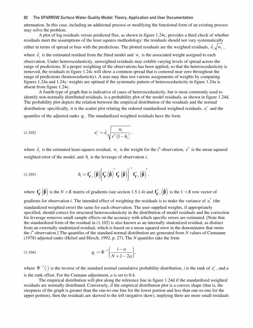
The SPARROW Surface Water-Quality Model: Theory, Application and User Documentation 92
attenuation. In this case, including an additional process or modifying the functional form of an existing process may solve the problem.
A plot of log residuals versus predicted flux, as shown in figure 1.24c, provides a third check of whether residuals meet the assumptions of the least squares methodology: the residuals should not vary systematically
either in terms of spread or bias with the predictions. The plotted residuals are the weighted residuals, i ie w ,
where is the estimated residual from the fitted model and is the associated weight assigned to each
observation. Under heteroscedasticity, unweighted residuals may exhibit varying levels of spread across the range of predictions. If a proper weighting of the observations has been applied, so that the heteroscedasticity is removed, the residuals in figure 1.24c will show a common spread that is centered near zero throughout the range of predictions (homoscedasticity). A user may thus test various assignments of weights by comparing figures 1.24a and 1.24c: weights are optimal if the systematic pattern of heteroscedasticity in figure 1.24a is absent from figure 1.24c.
ie iw
A fourth type of graph that is indicative of cases of heteroscedasticity, but is most commonly used to identify non-normally distributed residuals, is a probability plot of the model residuals, as shown in figure 1.24d. The probability plot depicts the relation between the empirical distribution of the residuals and the normal distribution: specifically, it is the scatter plot relating the ordered standardized weighted residuals, and the
quantiles of the adjusted ranks . The standardized weighted residuals have the form ie∗
iq
(1.102) ( )2
ˆ1i
i ii
we es h
∗ =−
,
where is the estimated least-squares residual, is the weight for the iie iwth observation, is the mean squared
weighted error of the model, and is the leverage of observation i,
2s
ih
(1.103) , ( ) ( ) ( ) ( )1
* * * *, ,
ˆ ˆ ˆ ˆi i ih
−
′ ′ ′ ′
⎛ ⎞′ ′⎟⎜ ⎟= ⎜ ⎟⎜ ⎟⎜⎝ ⎠β β β βf β f β f β f β
where is the N ×K matrix of gradients (see section 1.5.1.4) and ( )* ˆ′βf β ( )*
,ˆ
i′βf β is the 1 ×K row vector of
gradients for observation i. The intended effect of weighting the residuals is to make the variance of (the
standardized weighted error) the same for each observation. The user-supplied weights, if appropriately specified, should correct for structural heteroscedasticity in the distribution of model residuals and the correction for leverage removes small sample effects on the accuracy with which specific errors are estimated. [Note that the standardized form of the residual in (1.102) is also known as an internally studentized residual, as distinct from an externally studentized residual, which is based on a mean squared error in the denominator that omits the i
*ie
th observation.] The quantiles of the standard normal distribution are generated from N values of Cunnanne (1978) adjusted ranks (Helsel and Hirsch, 1992, p. 27). The N quantiles take the form
(1.104) 1
1 2ii aq
N a− ⎛ ⎞− ⎟⎜=Φ ⎟⎜ ⎟⎜⎝ ⎠+ −
,
where ( )1−Φ ⋅ is the inverse of the standard normal cumulative probability distribution, i is the rank of , and a
is the rank offset. For the Cunnane adjustment, a is set to 0.4. ie∗
The empirical distribution will plot along the reference line in figure 1.24d if the standardized weighted residuals are normally distributed. Conversely, if the empirical distribution plot is a convex shape (that is, the steepness of the graph is greater than the one-to-one line for the lower portion and less than one-to-one for the upper portion), then the residuals are skewed to the left (negative skew), implying there are more small residuals
Part 1: A Theoretical and Practical Introduction to SPARROW 93
and fewer large residuals compared to a normal distribution. If the empirical distribution is a concave shape (that is, the steepness of the graph is less than the one-to-one line for the lower portion and greater than one-to-one for the upper portion), then the residuals are skewed to the right (positive skew), implying there are more large residuals and fewer small residuals compared to a normal distribution. If the empirical distribution generally plots along the one-to-one line in the middle section of the graph but the tails of the figure show points consistently above or below the line, then there is more or less probability in the tails as compared to a normal distribution. For example, a group of points falling below the one-to-one line at the low end of the graph is indicative of an empirical distribution having a fatter left tail than the normal distribution. A group of points lying above the one-to-one line on the upper end of the graph is indicative of an empirical distribution that is fatter than the normal distribution in the right tail.
Because departure of the residuals distribution from normality does not necessarily invalidate the SPARROW model results, departures of the empirical distribution from the one-to-one line is not necessarily of concern. Failure to meet the three assumptions of the nonlinear least squares methodology (that residuals are mutually independent, identically distributed, and independent of the predictor variables) is, however, sometimes associated with deviations from the one-to-one line in the normal probability plot. For example, heteroscedasticity of the residuals (failure of the second assumption) causes the tails of the empirical distribution to be fatter than the normal distribution, which is expressed on the probability plot as points at the low end of the probability plot lying below the one-to-one line and points at the high end lying above the one-to-one line (as is the case for the residuals of the example nitrogen model shown in figure 1.24d). It is stressed, however, that heteroscedasticity represents a problem for model estimation and interpretation only if the heteroscedasticity is caused by failure of the third assumption, that is, if the residuals are related to the predictors (i.e., gradients). This particular cause of heteroscedasticity can be detected by interpreting the graph of predicted and observed flux in figure 1.24a.
The probability plot correlation coefficient provides a measure of the linear correlation between the ordered, standardized weighted residuals ( ), obtained from the estimated parametric model, and the quantiles
of the standard normal distribution ( ). A value of the correlation coefficient near one is evidence that the
residuals are from a normal distribution, whereas a value below 0.98 is generally indicative of non-normal residuals. A table of critical values for the normal probability plot correlation coefficient is given in Vogel (1986).
ie∗
iq
A formal test of the normality assumption is provided by the Shapiro-Wilk’s test statistic. The Shapiro-Wilks statistic takes the form
(1.105) W ′ ′= v x x Mx ,
where x is a vector of the weighted residuals ie wi ordered from low to high; M is the idempotent matrix
calculated as ( )′−I i i i i′ , where i is a vector of ones; and v is a vector of factors representing the normalized
values of the order statistics derived from a standard normal distribution
(1.106) 1 2− −′= m mv V m m V m ,
where m is the vector of order statistics from a standard normal distribution and is the covariance matrix of
m. The W statistic is essentially the squared value of the correlation coefficient between the residuals and the expected values of the normal order statistics. Because v is approximately proportional to the normal scores, W is a measure of the straightness of the normal probability plot. Probability values for evaluating the statistical significance of W are numerically estimated in SPARROW using an algorithm by Royston (1982). The standard SPARROW output includes the normal distribution probability plot correlation coefficient, the Shapiro-Wilks normality test statistic, and the probability value of the Shapiro-Wilks test statistic.
mV
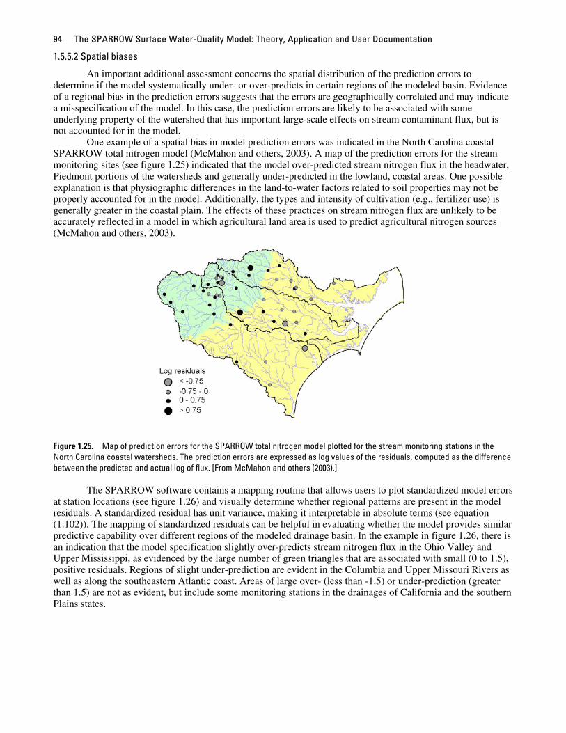
The SPARROW Surface Water-Quality Model: Theory, Application and User Documentation 94
1.5.5.2 Spatial biases
An important additional assessment concerns the spatial distribution of the prediction errors to determine if the model systematically under- or over-predicts in certain regions of the modeled basin. Evidence of a regional bias in the prediction errors suggests that the errors are geographically correlated and may indicate a misspecification of the model. In this case, the prediction errors are likely to be associated with some underlying property of the watershed that has important large-scale effects on stream contaminant flux, but is not accounted for in the model.
One example of a spatial bias in model prediction errors was indicated in the North Carolina coastal SPARROW total nitrogen model (McMahon and others, 2003). A map of the prediction errors for the stream monitoring sites (see figure 1.25) indicated that the model over-predicted stream nitrogen flux in the headwater, Piedmont portions of the watersheds and generally under-predicted in the lowland, coastal areas. One possible explanation is that physiographic differences in the land-to-water factors related to soil properties may not be properly accounted for in the model. Additionally, the types and intensity of cultivation (e.g., fertilizer use) is generally greater in the coastal plain. The effects of these practices on stream nitrogen flux are unlikely to be accurately reflected in a model in which agricultural land area is used to predict agricultural nitrogen sources (McMahon and others, 2003).
Figure 1.25. Map of prediction errors for the SPARROW total nitrogen model plotted for the stream monitoring stations in the North Carolina coastal watersheds. The prediction errors are expressed as log values of the residuals, computed as the difference between the predicted and actual log of flux. [From McMahon and others (2003).]
The SPARROW software contains a mapping routine that allows users to plot standardized model errors at station locations (see figure 1.26) and visually determine whether regional patterns are present in the model residuals. A standardized residual has unit variance, making it interpretable in absolute terms (see equation (1.102)). The mapping of standardized residuals can be helpful in evaluating whether the model provides similar predictive capability over different regions of the modeled drainage basin. In the example in figure 1.26, there is an indication that the model specification slightly over-predicts stream nitrogen flux in the Ohio Valley and Upper Mississippi, as evidenced by the large number of green triangles that are associated with small (0 to 1.5), positive residuals. Regions of slight under-prediction are evident in the Columbia and Upper Missouri Rivers as well as along the southeastern Atlantic coast. Areas of large over- (less than -1.5) or under-prediction (greater than 1.5) are not as evident, but include some monitoring stations in the drainages of California and the southern Plains states.
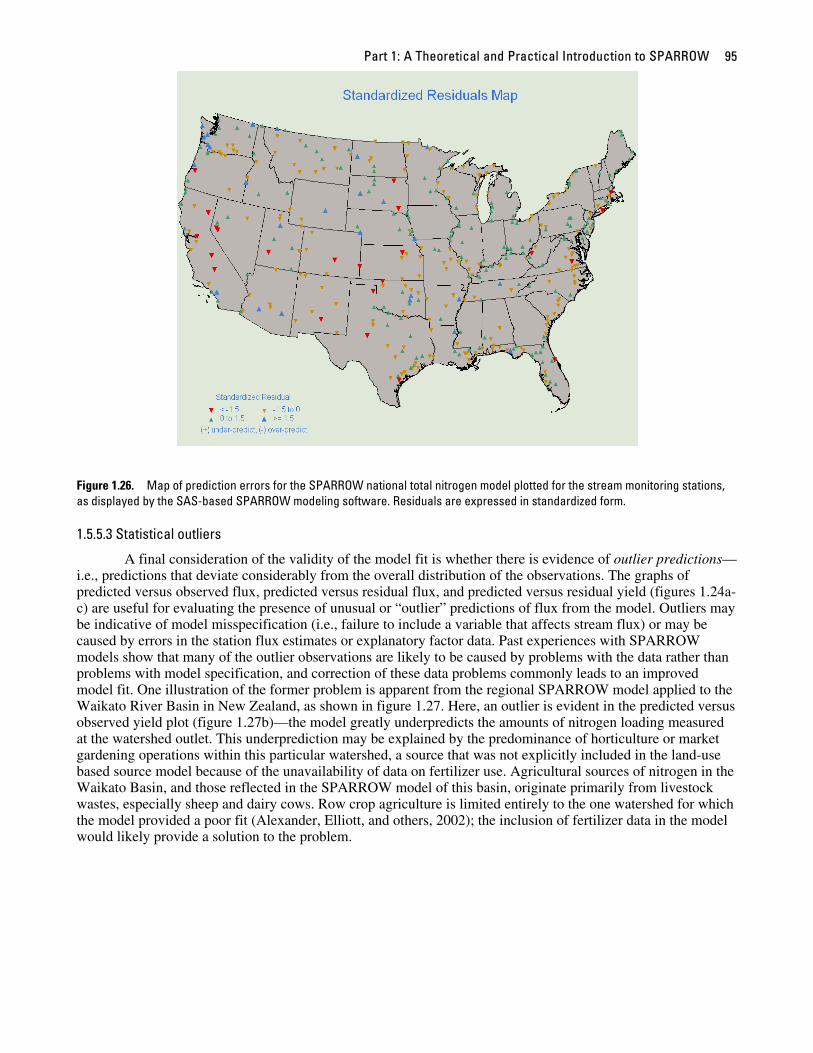
Part 1: A Theoretical and Practical Introduction to SPARROW 95
Figure 1.26. Map of prediction errors for the SPARROW national total nitrogen model plotted for the stream monitoring stations, as displayed by the SAS-based SPARROW modeling software. Residuals are expressed in standardized form.
1.5.5.3 Statistical outliers
A final consideration of the validity of the model fit is whether there is evidence of outlier predictions—i.e., predictions that deviate considerably from the overall distribution of the observations. The graphs of predicted versus observed flux, predicted versus residual flux, and predicted versus residual yield (figures 1.24a-c) are useful for evaluating the presence of unusual or “outlier” predictions of flux from the model. Outliers may be indicative of model misspecification (i.e., failure to include a variable that affects stream flux) or may be caused by errors in the station flux estimates or explanatory factor data. Past experiences with SPARROW models show that many of the outlier observations are likely to be caused by problems with the data rather than problems with model specification, and correction of these data problems commonly leads to an improved model fit. One illustration of the former problem is apparent from the regional SPARROW model applied to the Waikato River Basin in New Zealand, as shown in figure 1.27. Here, an outlier is evident in the predicted versus observed yield plot (figure 1.27b)—the model greatly underpredicts the amounts of nitrogen loading measured at the watershed outlet. This underprediction may be explained by the predominance of horticulture or market gardening operations within this particular watershed, a source that was not explicitly included in the land-use based source model because of the unavailability of data on fertilizer use. Agricultural sources of nitrogen in the Waikato Basin, and those reflected in the SPARROW model of this basin, originate primarily from livestock wastes, especially sheep and dairy cows. Row crop agriculture is limited entirely to the one watershed for which the model provided a poor fit (Alexander, Elliott, and others, 2002); the inclusion of fertilizer data in the model would likely provide a solution to the problem.
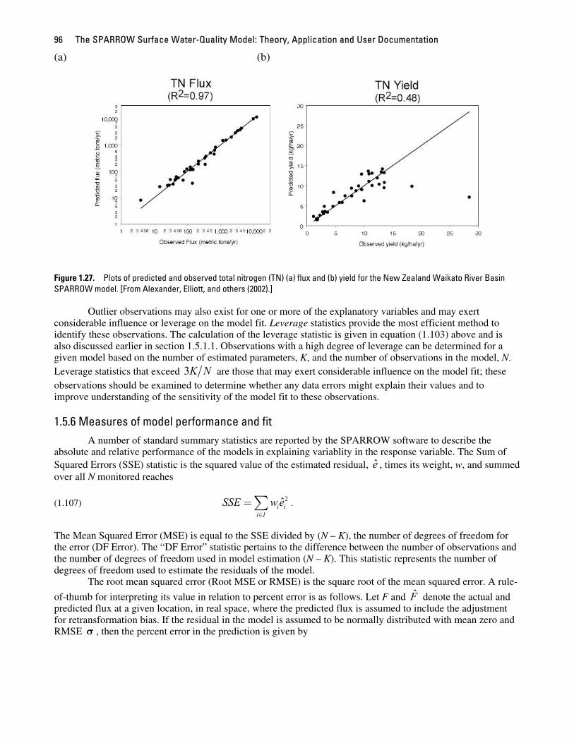
The SPARROW Surface Water-Quality Model: Theory, Application and User Documentation 96
(a) (b)
Figure 1.27. Plots of predicted and observed total nitrogen (TN) (a) flux and (b) yield for the New Zealand Waikato River Basin SPARROW model. [From Alexander, Elliott, and others (2002).]
Outlier observations may also exist for one or more of the explanatory variables and may exert considerable influence or leverage on the model fit. Leverage statistics provide the most efficient method to identify these observations. The calculation of the leverage statistic is given in equation (1.103) above and is also discussed earlier in section 1.5.1.1. Observations with a high degree of leverage can be determined for a given model based on the number of estimated parameters, K, and the number of observations in the model, N. Leverage statistics that exceed 3K N are those that may exert considerable influence on the model fit; these observations should be examined to determine whether any data errors might explain their values and to improve understanding of the sensitivity of the model fit to these observations.
1.5.6 Measures of model performance and fit A number of standard summary statistics are reported by the SPARROW software to describe the
absolute and relative performance of the models in explaining variablity in the response variable. The Sum of Squared Errors (SSE) statistic is the squared value of the estimated residual, , times its weight, w, and summed over all N monitored reaches
e
(1.107) . 2ˆi ii I
SSE we∈
=∑
The Mean Squared Error (MSE) is equal to the SSE divided by (N – K), the number of degrees of freedom for the error (DF Error). The “DF Error” statistic pertains to the difference between the number of observations and the number of degrees of freedom used in model estimation (N – K). This statistic represents the number of degrees of freedom used to estimate the residuals of the model.
The root mean squared error (Root MSE or RMSE) is the square root of the mean squared error. A rule-
of-thumb for interpreting its value in relation to percent error is as follows. Let F and denote the actual and predicted flux at a given location, in real space, where the predicted flux is assumed to include the adjustment for retransformation bias. If the residual in the model is assumed to be normally distributed with mean zero and RMSE , then the percent error in the prediction is given by
F
σ
Part 1: A Theoretical and Practical Introduction to SPARROW 97
(1.108) ( ) ( )2 2
ˆ100 100 1ˆ
F Fe
Fε σ−
−= − .
Consider the percent error in flux associated with a one standard deviation error, PE(σ ). We have,
(1.109) ( ) ( )2 2100 1 100PE eσ σσ σ−= − ≈ ,
where the approximation corresponds to a second-order Taylor expansion of the exponential term with respect to , which is approximately valid for all σ between 0 and 0.6. Thus, 100 times the RMSE approximately equals the percent error in the flux estimate, for any given reach, associated with a one standard deviation error. For greater than 0.6, the approximation is less precise and results in an overestimate of the percent error.
σ
σThe remaining fit statistics reported by the SPARROW software are R-square, adjusted R-square, and R-
square of the logarithm of contaminant yield. The R-square statistic (denoted 2R ) is given by (Judge and others, 1985, p. 30)
(1.110)
( )
2
2 1
2* *
1
1
N
ii
N
ii
eR
f f
=
=
= −−
∑
∑,
where ei is the model residual, in log space, for the ith observation, *if is the logarithm of measured flux for the
ith observation, and *f is the average of the *if over all N observations. Adjusted R-square applies a degrees of
freedom adjustment to the R-square statistic (Judge and others, 1985, p. 30)
(1.111) ( )2 21Adjusted 1 1NR RN K
⎛ ⎞− ⎟⎜= − −⎟⎜ ⎟⎜⎝ ⎠−.
The R-square and Adjusted R-Square statistics for a SPARROW model tend to be large (greater than 0.6). Large values for these statistics result partly from the fact that much of the variation in the dependent variable is associated with the size (drainage area) of the basin upstream from the monitored reach, and drainage area in turn is typically highly correlated with contaminant source variables. A high R-square, therefore, does not necessarily indicate the strength of the model within a smaller basin. Goodness of model fit for small basins might be better described by R-square of the logarithm of contaminant yield, denoted 2
YieldR . This statistic is
defined as
(1.112)
( ) ( )( )
2
2 12* *
1
1
N
ii
Yield N
i ii
eR
f f d d
=
=
= −− − −
∑
∑,
where di is the log of drainage area for the ith observation and d is the mean of di over all N observations. Because the log of drainage area is highly positively correlated with the log of flux, the denominator of the ratio term will be smaller than the corresponding term in the R-square equation, implying a smaller value for yield R-square.


![Asymptotic behavior of singularly perturbed control …€¦ · Asymptotic behavior of singularly perturbed control ... [Lions, Papanicolau, Varadhan 1986]; ... Asymptotic behavior](https://img.pdfslide.net/doc/110x75/5b7c19bc7f8b9a9d078b9b98/asymptotic-behavior-of-singularly-perturbed-control-asymptotic-behavior-of-singularly.jpg)