156-2010: Graph Elements You Should Know (Even If You Don ... · Not all of the graphics options will be utilized outside of the SAS/GRAPH environment, consequently you may need to

1

Paper 156-2010

SAS/GRAPH® Elements You Should Know – Even If You Don’t Use SAS/GRAPH

Arthur L. Carpenter

California Occidental Consultants ABSTRACT We no longer live or work in a line printer - green bar paper environment. Indeed many of today’s programmers do not even know what a line printer is or what green bar paper looks like. Our work environment expects reports which utilize various fonts, with control over point size and color, and the inclusion of graphic elements. In general we are expected to produce output that not only conveys the necessary information, but also looks attractive. In the line printer days little could be done with the style and appearance of reports, and consequently little was expected. Now a great deal of control is possible, and we are expected to take advantage of the tools available to us. We can no longer sit back and present a plain vanilla report. The Output Deliver System gives us a great deal of the kind of control that we must have in order to produce the kinds of reports and tables that are expected of us. Although we will often include graphical elements in our tables, it turns out that a number of options, statements, and techniques that are associated with SAS/GRAPH can be utilized to our benefit even when we are NOT creating graphs. Learn how to take advantage of these graphical elements, even when you are not using SAS/GRAPH. KEY WORDS SAS/GRAPH, ODS, GOPTIONS, SYMBOL, AXIS, TITLE USING TITLE OPTIONS WITH ODS For destinations that support font and color attributes, the Output Delivery System, ODS, honors many of the SAS/GRAPH title and footnote options. A few of the traditional TITLE/FOOTNOTE statement options include:

• Color= color designation • BColor= background color specification • Height= height of the text (usually specified in points) • Justify= text justification (left, center, right) • Font= font designation (can include hardware and software fonts)

Most of these options can be abbreviated. For the options shown above you can use the upper case letters in the option name as an abbreviation. Colors can include most standard color names as well as any of the RGB or gray scale colors appropriate for the output destination. There also a few font modification options. These include:

Hands-on WorkshopsSAS Global Forum 2010

2

• BOLD create bolded text • ITALIC italicize the text • UNDERLINE underline the text

The Base SAS® TITLE statement documentation does not mention any of these options. They are listed in the SAS/GRAPH documentation, however a number of the SAS/GRAPH TITLE statement options are not supported outside of the graphics environment. The following example demonstrates some of these TITLE statement options titles associated with a RTF report.

You may use any font available to your system. Fonts consisting of more than one word must be enclosed in quotes. The color is set to BLUE, and the font size is set to 15 points. This can be a fairly nominal size, as actual size can depend on the destination and how it is displayed. The background color is set to yellow. JUSTIFY=LEFT has been abbreviated.

The font is bolded. The options are applied to any text that follows the title option.

The RTF style has been used with the RTF destination, and when using the RTF style in the RTF destination changing the background color (BC=) adds a box around the title. In RTF the titles and footnotes are by default added to the HEADER and FOOTERS of the document when the table is imported. Footers are at the bottom of the physical page, and not necessarily at the bottom of the table. The titles/footnotes can be made a part of the

table itself through the use of the BODYTITLE option on the ODS RTF statement. For shorter tables this can move the footnote to the base of the table. There are quite a few other SAS/GRAPH TITLE statement options. Most of these are ignored outside of SAS/GRAPH. Depending on the destination and style, some SAS/GRAPH TITLE statement options are occasionally not ignored (when you think that they should be), in which case they tend to yield unanticipated results.

title1 f='times new roman' h=15pt c=blue bc=yellow 'Using TITLE Options'; ods rtf file="&path\results\E1.rtf" style=rtf; title2 f='Arial' h=13pt c=red j=l bold 'English Units'; proc report data=advrpt.demog nowd split='*'; . . . portions of the REPORT step not shown . . . .

ods rtf file="&path\results\E2.rtf" style=rtf bodytitle;


3

SETTING AND CLEARING GRAPHICS OPTIONS AND SETTINGS Most procedures that have graphics capabilities, can also take advantage of many graphics options and settings. Not all of the graphics options will be utilized outside of the SAS/GRAPH environment, consequently you may need to do some experimenting to determine which graphics options are used for the procedure of interest. Graphics options are set through the use of the GOPTIONS statement. Like the OPTIONS statement, this global statement is used to set one or more graphics options. Because there are a great many aspects to the preparation and presentation of a high resolution graphic, there are necessarily a large number of graphics options. A few of the more commonly used options are shown here.

Option Example Value

What it does

htext= 2.5 Sets the size for text border noborder

border Determines if a border is to be placed around the graphic?

device= emf Instruction set for the rendering of the graphic gsfname= fileref Location to write the file containing the graphic

Because these options and settings have a scope for the entire session, if you are in an interactive session and execute two or more programs that use or change some of these options, it is not

uncommon to have the options from one program interfere with those of the next. We can mitigate this by setting or resetting the graphic options to their default values at the

start of each program. This is done by using the RESET= graphics option. The RESET= graphics option can be used to reset a number of different groups of graphic settings. The following table shows some of these groups.

RESET= What it does

all resets all graphics options and settings. Resets values from some other statements as well (see below).

goptions only resets graphics options to their default values symbol clears all symbol statement definitions legend clears all legend statement definitions title clears all title definitions; same as title1; footnote clears all footnote definitions; same as footnote1;

goptions reset=symbol;


4

filename outex3 "&path\results\E3_goptions.emf"; goptions reset=all ftext='cambria' htext=1; GOPTIONS GSFNAME=outex3 GSFMODE=replace DEVICE=emf; *goptions device=win targetdevice=emf;

The following rather typical set of GOPTION statements utilizes some of the options shown above with a PROC UNIVARIATE step.

The RESET=all option clears all graphics options and sets them to their default values. The FTEXT option is used to set the default font for graphics text. CAMBRIA, a font with

serifs, is quite readable. Unless specified elsewhere, the HTEXT option sets the default height for all text to 1 unit. The default units are cells. Other choices include: IN, CM, PTS, PIXELS, PERCENT. Graphics Stream File options, GSF, are used to route the graph to a file. GSFNAME points to the destination, fileref, of the graphic GSFMODE, if the graphic file already exists it is to be replaced The DEVICE= option is used to structure the graph for the appropriate physical or virtual destination. EMF is a good device when the graphic is to be included in a word processing document

During program development you will want to see the graph displayed on the monitor (under windows this is DEVICE=WIN), however you may want to view it as it will ultimately be displayed on the final destination. The TARGETDEVICE option attempts to show you the graph on the display device (DEVICE=) using the constraints of the eventual final device

(TARGETDEVICE). Since this is a production example, this development statement has been commented out. USING SAS/GRAPH STATEMENTS WITH NON-SAS/GRAPH PROCEDURES In the previous example the UNIVARIATE procedure was used to generate a graph. Although UNIVARIATE is part of Base SAS, it can still take advantage of other aspects of SAS/GRAPH. It turns out that there are a number of other procedures, which although not part of SAS/GRAPH, are none-the-less able to take advantage of SAS/GRAPH statements when generating high resolution graphs. A few of the more common procedures that I have found to be useful that also have high resolution graphics capabilities include:

Using GOPTIONSPlots by PROC UNIVARIATE

024681012

Count

Mean: 144.55

F

100 115 130 145 160 175 190 205 220 235 250024681012

Count

Mean: 172.91

M

weight in pounds

patient sex


5

Base UNIVARIATE SAS/QC CAPABILITY SHEWART SAS/STAT BOXPLOT PROBIT REG The following is a very brief introduction to some of the statements that can be used outside of SAS/GRAPH. Better and more complete introductions to SAS/GRAPH can be found in numerous papers, as well as in several books. Although outside the scope of this paper, ODS Stat Graphics can also be used to generate high resolution graphics. Changing Plot Symbols with the SYMBOL Statement The SYMBOL statement is used to control the appearance of items within the graphics area. As you would suspect, this includes plot symbols, but it also controls the appearance of lines, and how points are joined with these lines. All plot symbols and lines have attributes e.g. color, size, shape, thickness, and these attributes are declared on the SYMBOL statement. There can be up to 99 numbered SYMBOL statements. Attributes to be controlled are specified through

the use of options. Options are specified through the use of their name and, in most cases, the names can be abbreviated. The

following SYMBOL statement requests that the plot symbols (a dot) be blue, with a size (height) of .8 units. Fortunately, since the SYMBOL statement is heavily used, it is usually fairly straight forward to apply. A quick study of the documentation will usually serve as a first pass instruction. Like so many things in SAS however, there are a few traps that you should be aware of when applying the SYMBOL statement in more complex situations.

symbol1 color = blue h = .8 v=dot;


6

A few of the numerous SYMBOL statement options are shown in the following table.

Option Option Abbreviation

Example Value

What it does

color= c= blue Sets the color of the symbol and/or line height= h= 1.5 Size of the symbol value= v= star Symbol to be used in the plot font= f= arial The plot symbol is selected from this font interpol= i= join How plot symbols are to be connected line= l= 1 Line numbers: 1, 2 , and 33 are the most useful width= w= 2.1 Line width, the default is usually 1

SYMBOL Definitions are Cumulative Although SYMBOL statements, like TITLE and FOOTNOTE statements, are numbered, that is about the only similarity with regards to the way that the definitions are established. When a TITLE3 statement is specified, the definition for TITLE3 is completely replaced. Not only is a given TITLE statement the complete definition for that title, but that same TITLE3 statement automatically clears titles 4 though 10; SYMBOL statement definitions, on-the-other-hand, are cumulative. The following two SYMBOL statements could be rewritten as several statements.

The graphics option RESET= can be used in the GOPTIONS statement to clear SYMBOL statement

definitions.

SYMBOL Definition Selection is NOT User Directed When symbols or lines are to be used in a graph, the procedure first checks to see if there are any user defined symbol definitions (of course, there are defaults for everything when SYMBOL statements have not been used). The procedure then selects the next symbol definition. This means that if SYMBOL2 was just used, the procedure will look for a SYMBOL3 definition. Unfortunately it is not possible to directly tie a given symbol statement to a given line or symbol. This means that you will need to have at least a basic understanding of symbol definition selection for the procedure that you are planning on using. The following example uses PROC REG to perform a regression analysis on HT and WT in the DEMOG data set. The PLOT statement can be used to create a plot of the results of the analysis.

symbol1 color = blue v=none i=box10 bwidth=3; symbol2 color = red v=dot i=join line=2 h=1.2;

symbol2 v=dot i=join; symbol1 color = blue; symbol2 color = red; symbol1 v=none i=box10 bwidth=3; symbol2 line=2 h=1.2;

goptions reset=symbol;


7

All graphics options are set to their defaults. Then selected options are changed as in the previous example. TITLE statement options are used to select bolded arial as the font for the first title. HT is used as the dependent variable. The CONF option is

used to request the plotting of the confidence intervals and predicted values. Although the procedure selects colors and line types for the predicted value line and for the confidence intervals, the data are plotted using the plus ‘+’ symbol. In this case the predicted line is red, upper confidence bound is yellow and the lower limit is green. We can use the SYMBOL statement to

gain control of the plot symbol and the color of the lines.

goptions reset=all device=emf gsfname=outex4a noprompt htext=1 ftext='cambria' title1 f=arial bold 'Regression of HT and WT'; title2 'No SYMBOL Statement'; proc reg data=advrpt.demog; model ht = wt; plot ht*wt/conf; run; quit;

ht = 58.823 +0.0541 wt N 77 Rsq 0.2985AdjRsq0.2891RMSE 2.951

Regression of HT and WTNo SYMBOL Statement

height in inch

es

62646668707274

weight in pounds80 100 120 140 160 180 200 220 240Plot ht*wt PRED*wt L95M*wt U95M*wt


8

For the data points the SYMBOL1 statement is used to select the plot symbol, color, and

the symbol (V=). The color for the estimated line is specified. You will need to experiment to determine which SYMBOL statement will be used by which aspect of the graph. The confidence lines are colored green. The R= option causes this symbol definition to be reused a second time. Rather than use the R= option we could have specified a SYMBOL4

definition to be the same as the SYMBOL3 definition. The colors and plot symbols are shown in the legend at the bottom of the graph. You can take control of the legend though the use of the LEGEND statement. Although not supported by REG, for some procedures you can eliminate the legend altogether using the NOLEGEND option. Controlling Axes and Legends Control of any and all aspects of the horizontal and vertical axes can be obtained through the use of the AXIS statement. This global statement can be one of the most complex statements in SAS/GRAPH, if not within SAS itself, and it is clearly outside of the scope of this paper to do much more than partially describe this statement. Closely related to the AXIS statement in syntax is the LEGEND statement which is used to control the appearance of the graph’s legend. The following is a brief introduction to these two statements. Like the SYMBOL statement, you can have up to 99 numbered AXIS and LEGEND statements. Also like

the SYMBOL statement, the axis and legend definitions are cumulative. Both axis and legend definitions can be cleared with the RESET= option.

title2 'With SYMBOL Statements'; symbol1 c=blue v=dot; symbol2 c=red; symbol3 c=green r=2;

goptions reset=axis; goptions reset=legend;


Regression of HT and WTWith SYMBOL Statements

height in inch

es

62646668707274

weight in pounds80 100 120 140 160 180 200 220 240Plot ht*wt PRED*wt L95M*wt U95M*wt


9

AXIS Statement The AXIS statement can be used to control the axis lines, tick marks, tick mark text, and axis labels. You can specify fonts and color for all text. For any of the lines you can control the styles (type of line), thickness, color, and length. The axis definition is built through a series of options. Some of these options will themselves have options, and the layers of options within options can often be three deep. To make things even more interesting some options will appear in multiple ways and their effect will depend on position and usage. Clearly just knowing how to apply the options and how to nest them can be complicated. Most of the options that can appear in several different aspects of the statement are text appearance options. Most are similar to those used as TITLE and FOOTNOTE statement options, and there is also some overlap with those used in the SYMBOL statement. Some of the more common text appearance options include:

Option Option Abbreviation

Example Value

What it does

height= h= 10pct size is set to 10 percent color= c= cxdedede color is set to a shade of gray font= f= Arial ARIAL is selected as the desired font ‘text string’ ‘Units are mg’

The first layer of options control major aspects of the axis. These include such things as:

• ORDER= range of values to be included • LABEL= axis label • VALUE= tick mark control • MAJOR= major tick marks (the ones with text) • MINOR= minor tick marks

When building an AXIS statement parentheses are used to form groups of sub-options, and indenting to each level of option can be helpful in keeping track of which options go with what. This is a fairly typical

AXIS statement. Notice that the values of options are in parentheses. This allows us to specify the sub-options. ORDER= Restricts the axis range, data can be excluded. Here the range of the axis is limited to values between 75 and

250 with major tick marks at an interval of 25. H= The height of the text is set to 1.5 units (the default units are cells) Color= The color for the label text is set to blue ‘text’ The text for the label is specified overriding the variable’s label MINOR= Specifies the number of minor tick marks. Eliminate all with MINOR=NONE.

axis1 order=(75 to 250 by 25) label=(h=1.5 c=blue 'Weight (LB)') value=(h=1.5) minor=(n=4) color=red;


10

Since the Color= option is not within parentheses, RED will become the default color for all aspects of the axis. The following box plot uses the previous axis statement to control a few of the aspects of the vertical axis.

For most procedures a given AXIS statement is associated with the vertical or horizontal axis through the use of options on the statement that defines the plot. In PROC BOXPLOT, which was used here, the defining statement is the PLOT statement and there is a both a VAXIS= and HAXIS= option to assign the axis statement. Since in this example the vertical axis is associated with the AXIS1 statement, the option would be

VAXIS=AXIS1. The BOXPLOT step becomes:

LEGEND Statement The general syntax, statement structure, and even many of the options of the AXIS statement

are shared with the LEGEND statement. In the discussion of the use of the SYMBOL statement with the regression plot earlier in this paper, the legend appears at the bottom of the graph. We can change its location as well as its appearance. The legend can be INSIDE or OUTSIDE of the graphics area, and it can also be moved vertically and horizontally.

legend1 position=(top left inside) value=(f='arial' t=1 'Height' t=2 'Predicted' t=3 'Upper 95' t=4 'Lower 95') label=none frame across=2; proc reg data=advrpt.demog; model ht = wt; plot ht*wt/conf legend=legend1; run;

PROC BOXPLOTWith Vertical AXIS Statement

01 02 03 04 05 06 09 1075100125150175200225250

Weight (LB)

symptom code

1122

proc boxplot data=demog; plot wt*symp/ cframe = cxdedede boxstyle = schematicid cboxes = red cboxfill = cyan vaxis = axis1 ; id race; run;


11

The VALUE= option controls the text associated with the four individual items in the legend. Turn off the legend’s label. Add a box around the legend. Other options allow you to change the width, color, and shadowing of the frame.

Allow at most 2 items for each row in the legend. The LEGEND= option is used to identify the appropriate legend statement. For this graph, especially when displayed in black and white, the legend is fairly superfluous. Many procedures have an option (NOLEGEND) that can be used to prevent the display of the legend altogether. Unfortunately PROC REG does not support the NOLEGEND option.

Consequently there is no way to prevent the legend from appearing when any of the PLOT statement options are used that cause multiple items to be displayed (such as CONF). The following example uses a LEGEND statement to minimize the impact of the legend.

The text for the individual values and the label is turned off. The individual symbol elements cannot be turned off (SHAPE does not support NONE), therefore the values are made very small.

Move the legend to the lower right corner where it will be less noticeable. The LEGEND2 definition is selected for use.

legend2 label=none value= none shape=symbol(.001,.001) position=(inside bottom right); proc reg data=advrpt.demog; model ht = wt; plot ht*wt/conf legend=legend2; run;


Regression of HT and WTUsing a LEGEND Statement

height in inch

es

62646668707274

weight in pounds80 100 120 140 160 180 200 220 240

Height PredictedUpper 95 Lower 95


Regression of HT and WTEliminating the Legend

height in inch

es

62646668707274

weight in pounds80 100 120 140 160 180 200 220 240


12

USING ANNOTATE TO AUGMENT GRAPHS The annotate facility gives us the ability to customize the output generated by the procedure. Although designed to be used with the graphics procedures in SAS/GRAPH, it can be used with a number of other procedures that generate graphics output. The huge advantage to us is that the customization provided by annotate can be data dependent. This means that without recoding, our graphs can change as the data changes. The key to the process is the annotate data set. This data set contains the instructions that are to be passed to the annotate facility. Each observation in the data set is one instruction, and very often the instruction is fairly primitive e.g. pick up a pen. The instructions in the data set are passed to the procedure that is generating the graphic through the use of the ANNOTATE= option. You can tell if a procedure can take advantage of the annotate facility by whether or not it supports this option or its abbreviation ANNO=. The annotate facility interprets each observation in the annotate data set as an instruction, and it uses the values of specific variables to form the intent of the instruction. You do not get to choose the names of the variables, but you have a great deal to do with the values that the variables take on. In order for the instruction to provide a valid instruction to annotate, the variables and their values have to provide answers to three primary questions.

Question to be answered Possible variables used to answer the question

WHAT is to be done? FUNCTION (this is the only variable for this question) WHERE is it to be done? X, Y, XSYS, YSYS HOW is it to be done? COLOR, SIZE, STYLE, POSITION

The value of the variable FUNCTION is always specified, and this value determines what other variables will be used by annotate when the instruction is executed. FUNCTION should be a character variable with a length of 8. There are over two dozen possible values for FUNCTION, a few of the commonly used ones are shown here.

Value of FUNCTION What it does

label Adds a text label to the graphic move Moves the pointer to another position on the graphic without drawing draw Draw a line from the current position to a new position on the graphic

For annotate operations that are associated with a location on a graphic, separate variables are used to specify the location. In order to identify a location you will need to specify the coordinate system (e.g. XSYS, YSYS) and a location within that coordinate system (e.g. X, Y).


13

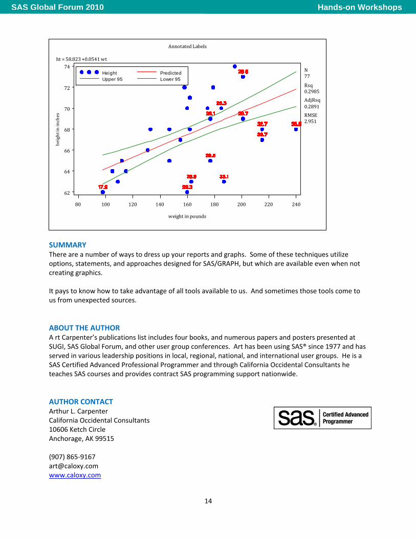
In this example the Body Mass Index, BMI, is calculated and then added to the regression plot generated by REG using the annotate facility. The annotate data set is named as are the variables that it will contain. The annotate variables FUNCTION and COLOR are assigned a length. To avoid truncation; this is always a good idea. The annotate variables that are constant for all the instructions (observations) are assigned values with the RETAIN. Only create an annotate instruction, a label, for those observations with a BMI outside of the stated range.

The variables X and Y contain the coordinates of this data point on the graph. TEXT, the variable used to hold the annotate label, contains the value of the BMI.

Write this annotate instruction to the annotate data set. The ANNO= option is used to name the data set containing the annotate instructions. An introduction to the annotate facility can be found in Annotate Simply the Basics (1999).

data bmilabel(keep=function xsys ysys x y text color style position size); set grphdata.demog; * Define annotate variable attributes; length color function $8; retain function 'label' xsys ysys '2' color 'red' style 'swissb' position '2' size .8; * Calculate the BMI. Note those outside of * the range of 18 - 26; bmi = wt / (ht*ht) * 703; if bmi lt 18 or bmi gt 26 then do; * Create a label; text = put(bmi,4.1); x=wt; y=ht; output bmilabel; end; run;

proc reg data=advrpt.demog; model ht = wt; plot ht*wt/conf legend=legend1 anno=bmilabel; run;


14

SUMMARY There are a number of ways to dress up your reports and graphs. Some of these techniques utilize options, statements, and approaches designed for SAS/GRAPH, but which are available even when not creating graphics. It pays to know how to take advantage of all tools available to us. And sometimes those tools come to us from unexpected sources. ABOUT THE AUTHOR A rt Carpenter’s publications list includes four books, and numerous papers and posters presented at SUGI, SAS Global Forum, and other user group conferences. Art has been using SAS® since 1977 and has served in various leadership positions in local, regional, national, and international user groups. He is a SAS Certified Advanced Professional Programmer and through California Occidental Consultants he teaches SAS courses and provides contract SAS programming support nationwide. AUTHOR CONTACT Arthur L. Carpenter California Occidental Consultants 10606 Ketch Circle Anchorage, AK 99515 (907) 865-9167 [email protected] www.caloxy.com


Annotated Labelsheight

in inches

62646668707274

weight in pounds80 100 120 140 160 180 200 220 240

Height PredictedUpper 95 Lower 95


15

REFERENCES Carpenter Arthur L. and Charles E. Shipp, 1995, Quick Results with SAS/GRAPH® Software, Cary, NC: SAS Institute Inc., 249 pp. http://www.sas.com/apps/pubscat/bookdetails.jsp?catid=1&pc=55127 Carpenter, Arthur L., 1999, Annotate: Simply the Basics, SAS Institute, Inc., Cary, NC. http://www.sas.com/apps/pubscat/bookdetails.jsp?catid=1&pc=57320 Haworth, Lauren, Cynthia L. Zender, and Michele Burlew, 2009, Output Delivery System: Basics and Beyond, SAS Institute, Inc., Cary, NC. http://www.sas.com/apps/pubscat/bookdetails.jsp?catid=1&pc=61686 TRADEMARK INFORMATION SAS, SAS Certified Professional, SAS Certified Advanced Programmer, and all other SAS Institute Inc. product or service names are registered trademarks of SAS Institute, Inc. in the USA and other countries. ® indicates USA registration.


Documents

156-2010: Graph Elements You Should Know (Even If You Don ... · Not all of the graphics options will be utilized outside of the SAS/GRAPH environment, consequently you may need to