156 c©Perry Y.Li

Chapter 6

Linear Quadratic Optimal Control

6.1 Introduction

In previous lectures, we discussed the design of state feedback controllers using using eigenvalue(pole) placement algorithms. For single input systems, given a set of desired eigenvalues, thefeedback gain to achieve this is unique (as long as the system is controllable). For multi-inputsystems, the feedback gain is not unique, so there is additional design freedom. How does oneutilize this freedom? A more fundamental issue is that the choice of eigenvalues is not obvious. Forexample, there are trade offs between robustness, performance, and control effort.

Linear quadratic (LQ) optimal control can be used to resolve some of these issues, by notspecifying exactly where the closed loop eigenvalues should be directly, but instead by specifyingsome kind of performance objective function to be optimized. Other optimal control objectives,besides the LQ type, can also be used to resolve issues of trade offs and extra design freedom.

We first consider the finite time horizon case for general time varying linear systems, andthen proceed to discuss the infinite time horizon case for Linear Time Invariant systems.

6.2 Finite Time Horizon LQ Regulator

6.2.1 Problem Formulation

Consider the m− input, n−state system with x ∈ <n, u ∈ <m:

x = A(t)x+B(t)u(t); x(0) = x0. (6.1)

Find open loop control u(τ), τ ∈ [t0, tf ] such that the following objective function is minimized:

J(u, x0, t0, tf ) =

∫ tf

t0

[xT (t)Q(t)x(t) + uT (t)R(t)u(t)

]dt+ x(tf )TSx(tf ). (6.2)

where Q(t) and S are symmetric positive semi-definite n×n matrices, R(t) is a symmetric positivedefinite m×m matrix. Notice that x0, t0, and tf are fixed and given data.

The control goal generally is to keep x(t) close to 0, especially, at the final time tf , using littlecontrol effort u. To wit, notice in (6.2)

• xT (t)Q(t)x(t) penalizes the transient state deviation,

• xT (tf )Sx(tf ) penalizes the final state

157

158 c©Perry Y.Li

• uT (t)R(t)u(t) penalizes control effort.

This formulation can accommodate regulating an output y(t) = C(t)x(t) ∈ <r at near 0. In thiscase, one choice for S and Q(t) are CT (t)W (t)C(t) where W (t) ∈ <r×r is symmetic positive definitematrix.

6.2.2 Solution to optimal control problem

General finite, fixed horizon optimal control problem: For the system with fixed initialcondition,

x = f(x, u, t); x(t0) = x0 given,

and a given time horizon [t0, tf ], find u(t), t ∈ [t0, tf ] such that the following cost function isminimized:

J(u(·), x0) = φ(x(tf )) +

∫ tf

t0

L(x(t), u(t), t)dt

where the first term is the final cost and the second term is the running cost.

Solution:

λ = −Hx = −∂L∂x− λT ∂f

∂x(6.3)

x = f(x, u, t) (6.4)

Hu = −∂L∂u− λT ∂f

∂u= 0 (6.5)

λT (tf ) =∂φ

∂x(x(tf )) (6.6)

x(t0) = x0. (6.7)

This is a set of 2n differential equations (in x and λ) with split boundary conditions at t0 and tf :x(t0) = x0 and λT (tf ) = φx(x(tf )), and an equation that would typically specify u(t) in terms ofx(t) and/or λ(t). We shall see the specialization to the LQ case soon.

Proof: The solution is obtained by converting the constrained optimal control problem into anunconstrained optimal control problem using the Lagrange multiplier function λ(t) ∈ <n:

J(u, x0) = J(u(·), x0) +

∫ tf

t0

λT (t)[f(x, u, t)− x]dt.

Note that ddt(λ

T (t)x(t)) = λT (t)x(t) + λT (t)x. So∫ tf

t0

λT x dt = λT (tf )x(tf )− λT (t0)x(t0)−∫ tf

t0

λTx dt.

Let us define the so called Hamiltonian function H(x, u, t) := L(x, u, t) + λT (t)f(x, u, t). Thus,

J = φ(x(tf ))− λT (tf )x(tf ) + λT (t0)x(t0) +

∫ tf

t0

[H(x(t), u(t), t) + λ(t)x(t)

]dt

The necessary condition for optimality is that the variation δJ of the modified cost with respectto all feasible variations δx(t), δλ(t), δu(t) and δλ(tf ) should vanish.

University of Minnesota ME 8281: Advanced Control Systems Design, 2001-2012 159

δJ = [φx − λT ]δx(tf ) + λT (t0)δx(t0) +

∫ tf

t0

{[Hx + λT ]δx(t) + [Hu]δu(t)

}dt

+

∫ tf

t0

δλT (t)[f(x(t), u(t), t)− x]dt

Since x(t0) = x0 is fixed, δx(t0) = 0. Otherwise, other variations δx(t), δu(t) or δλ(t) are allfeasible. Setting the terms that multiply these variations to be zero yield Eqs.(6.3)-(6.6). �

6.2.3 Open loop solution

Applying the general optimal control solution in section 6.2.2 to the LQ problem in Eqs.(6.1)-(6.2),we have:

Theorem 6.2.1 The optimal control is given by:

uo(t) = −R−1BT (t)λ(t) (6.8)

where λ(t) and x(t) satisfy the Hamilton-Jacobi equation:(x

λ

)=

(A(t) −B(t)R−1BT (t)−Q(T ) −AT (t)

)︸ ︷︷ ︸

Hamiltonian Matrix - H(t)

(xλ

)(6.9)

with boundary conditions:x(t0) = x0; λ(tf ) = Sx(tf ). (6.10)

• Boundary conditions are specified at both initial time t0 and final time tf (two point boundaryvalue problem). In general, these are difficult to solve and require iterative methods such asshooting method.

• Optimal control in Eq. (6.8) is open loop. It is computed by first computing λ(t) for allt ∈ [t0, tf ] and then applying uo(t) = −R−1BT (t)λ(t).

• Open loop control is not robust to disturbances or uncertainties.

6.2.4 Feedback control solution

Consider the matrix differential equation using the Hamiltonian matrix H(t), where X1(t), X2(t) ∈<n×n. (

X1(t)

X2(t)

)=

(A(t) −B(t)R−1BT (t)−Q(T ) −AT (t)

)︸ ︷︷ ︸

Hamiltonian Matrix - H(t)

(X1(t)X2(t)

)(6.11)

with boundary conditions X1(tf ) ∈ <n×n being any invertible matrix, and

X2(tf ) = SX1(tf ).

X1(t) and X2(t) can be integrated backwards in time from tf → t0.

160 c©Perry Y.Li

Let us assume (and it can be proven) that X1(t) is invertible. We propose that the solution tothe Hamilton-Jacobi equation (6.9)-(6.10) is given by:(

x(t)λ(t)

)=

(X1(t)X2(t)

)v

for some constant vector v.x(t) and λ(t) as proposed clearly satisfy (6.9), and the boundary condition λ(tf ) = Sx(tf ). The

initial condition x(t0) = x0 can be satisfied by choosing v = X−11 (t0)x0.If we define P (t) = X2(t)X

−11 (t), then λ(t) = P (t)x(t), so that the optimal control in Eq. (6.8)

can be implemented as a feedback as given in the following theorem.

Theorem 6.2.2 The cost function (6.2) is minimized using the control:

u∗(t) = −R(t)TBT (t)P (t)x(t) (6.12)

where P (t) ∈ <n×n is the solution to the following so called continuous time Riccati DifferentialEquation (CTRDE):

−P (t) = AT (t)P (t) + P (t)A(t)− P (t)B(t)R−1(t)BT (t)P (t) +Q(t); P (tf ) = S. (6.13)

Moreover, the minimum cost achieved using the above control is:

J∗(x0, t0, tf ) := minu(·)J(u, x0) = xT0 P (t0)x0

Proof: The feedback form of the optimal control Eq.(6.12) has already been shown. To showthat CTRDE in Eq.(6.13) is satisfied by P (t), one needs only differentiate P (t) = X−11 (t)X2(t),and making use of Eq.(6.11) and its boundary conditions.

The proof that P (t) determines the minimal cost will be discussed later using Dynamic Pro-gramming (DP) principle. �

Remarks

1. P (t) is solved backwards in time from tf → t0 and should be stored in memory before use.

2. The optimal control law is in the form of a time varying linear state feedback u(t) = −K(t)x(t)with feedback gain K(t) := R(t)TBT (t)P (t). The open loop optimal control can be obtained,if so desired, by integrating (6.1) with the control (6.12). It is, however, much better to utilizefeedback than to use openloop.

3. The Riccati differential equation can be derived from P (t) = X2(t)X−11 (t) and (6.11).

4. By direct substitution, it is easy to see the solution λ(t) = P (t)x(t) satisfies (6.9)-(6.10).Since the solution of CTRDE (6.13) does not rely on solving for X1(t) or X2(t) explicitly, theassumption that X1(t) is invertible is in fact not needed for the proof of this theorem. It canbe thought of as a useful device to guess the solution.

5. The control formulation works for time varying systems, e.g. nonlinear systems linearizedabout a trajectory.

6. P (t) can be shown to be associated with the cost-to-go function (see below). Using thisinterpretation, it can easily be shown that P (t) must be at least positive semi-definite.

University of Minnesota ME 8281: Advanced Control Systems Design, 2001-2012 161

6.2.5 Cost-to-go function

The matrix function P (t) is associated with the so-called cost-to-go function. By this it is meantthat if at any time t1 ∈ [t0, tf ], and the state is x(t1), then, the control policy (6.12) for theremaining time period [t1, tf ] will result in a cost J(u, x(t1), t1, tf ) in (6.2) with t0 substituted byt1 and x0 substituted by x(t1) such that:

Jo(x(t), t, tf ) := minuJ(u, x(t), t, tf ) = xT (t)P (t)x(t)

Since the optimal control, uo(t) = −K(t)x(t) = −R−1(t)BT (t)P (t)x(t), the closed loop systemsatisfies,

x = [A(t)−B(t)K(t)]x(t)

so that x(t) = Φ(t, t0)x0 where Φ(t, t0) is the transition matrix for A(t)−B(t)K(t). For this reason,the achieved minimal cost function must be of the form (omitting final time tf to avoid clutter):

Jo(x0, t0) = J(uo, x0, t0, tf ) = xT0 P (t0)x0.

for some positive semi-definite matrix P (t0). Our task is to show that P (t0) = P (t0). To derivethis result, we need the dynamic Programming (DP) Principle.

6.3 Dynamic Programming Principle

Consider the system:x = f(x(t), u(t), t), x(t0) = x0,

and the cost index over the interval [t0, tf ] is:

J(u(·), x0, t0) =

∫ tf

t0

L(x(t), u(t), t)dt+ φ(x(tf )). (6.14)

In the theorem below, tf is assumed to be fixed.

Theorem 6.3.1 Suppose that uo(t), t ∈ [t0, tf ] minimizes (6.14) subject to xo(t0) = x0 and xo(t)is the associated state trajectory. Let the (minimum) cost achieved using uo(t) be:

Jo(x0, t0) = arg minu(τ),τ∈[t0,tf ]

J(u(·), xo, t0, tf )

Then, for any t1 s.t. t0 ≤ t1 ≤ tf , the restriction of the control uo(τ) to τ ∈ [t1, tf ] minimizes

J(u(·), xo(t1), t1) =

∫ tf

t1

L(x(t), u(t), t)dt+ φ(x(tf ))

subject to the initial condition x(t1) = xo(t1). i.e. uo(τ) is optimal over the sub-interval [t1, tf ].

Corollary 6.3.2 Let t0 ≤ t1 ≤ tf . Consider the optimal control problem for the sub-interval [t1, tf ].If Jo(x0, t1) is the optimal cost and the optimal control is given by u(t) = uo(x0, t) for t ∈ [t1, tf ].Then, the optimal control for the larger interval t ∈ [t0, tf ] with initial condition x(t0) = x0 is givenby:

u(t) =

{arg minu(·)

∫ t1t0L(x, u, t)dt+ Jo(x(t1), t1) t ∈ [t0, t1)

uo(x(t1), t) t ∈ [t1, tf ](6.15)

where x(t1) is the state attained via the control u(t) above.

162 c©Perry Y.Li

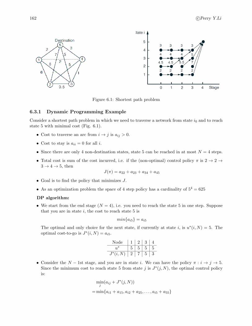
Figure 6.1: Shortest path problem

6.3.1 Dynamic Programming Example

Consider a shortest path problem in which we need to traverse a network from state i0 and to reachstate 5 with minimal cost (Fig. 6.1).

• Cost to traverse an arc from i→ j is aij > 0.

• Cost to stay is aii = 0 for all i.

• Since there are only 4 non-destination states, state 5 can be reached in at most N = 4 steps.

• Total cost is sum of the cost incurred, i.e. if the (non-optimal) control policy π is 2 → 2 →3→ 4→ 5, then

J(π) = a22 + a23 + a34 + a45

• Goal is to find the policy that minimizes J .

• As an optimization problem the space of 4 step policy has a cardinality of 54 = 625

DP algorithm:

• We start from the end stage (N = 4), i.e. you need to reach the state 5 in one step. Supposethat you are in state i, the cost to reach state 5 is

min{ai5} = ai5

The optimal and only choice for the next state, if currently at state i, is u∗(i,N) = 5. Theoptimal cost-to-go is J∗(i,N) = ai5.

Node 1 2 3 4

u∗ 5 5 5 5

J∗(i,N) 2 7 5 3

• Consider the N − 1st stage, and you are in state i. We can have the policy π : i → j → 5.Since the minimum cost to reach state 5 from state j is J∗(j,N), the optimal control policyis:

minj

(aij + J∗(j,N))

= min{ai1 + a15, ai2 + a25, . . . , ai5 + a55}

University of Minnesota ME 8281: Advanced Control Systems Design, 2001-2012 163

For i = 4 (for instance),

j 1 2 3 4

a4j 2 5 1 0

a4j + J∗(j,N) 4 11 6 3

Thus, the j the optimizes this is: j = 4 (stay put) so that u∗(4, N−1) = 4 and J∗(4, N−1) = 3.Doing this for each i, we have at stage N − 1,

– Optimal policy:u∗(i,N − 1) = argmin

j(aij + J∗(j,N))

– Optimal cost-to-go:J∗(i,N − 1) = min

j(aij + J∗(j,N))

Node 1 2 3 4

u∗(i,N − 1) 1 3 4 4

J∗(i,N − 1) 2 5.5 4 3

• If we are at the N − 2nd stage, and you are in state i,

– Optimal policy:u∗(i,N − 2) = arg min

j(aij + J∗(j,N − 1))

– Optimal cost-to-go:J∗(i,N − 2) = min

j(aij + J∗(j,N − 1))

Node 1 2 3 4

u∗(i,N − 2) 1 3 3 4

J∗(i,N − 2) 2 4.5 4 3

Notice that from state 2, the 3 step policy

2→ 3→ 4→ 5

has a lower cost of 4.5 than the 2 step policy 2→ 3→ 5 with a cost of 5.5.

• Repeating the propagation procedure for the optimal policy and optimal cost-toabove untilN = 1. Then the optimal policy is u∗(i, 1) and the minimum cost is J∗(i, 1).

• The optimal sequence starting at i0 is:

i0 → u∗(i0, 1)→ u∗(u∗(i0, 1), 2)

→ u∗(u∗(u∗(i0, 1), 2), 3)→ 5

Remarks:

• At each stage k, the optimal policy u∗(i, k) is a state feedback policy. i.e. it determines whatto do depending on the state that you are in.

164 c©Perry Y.Li

• Policy and optimal cost-to-go are computed backwards in time (stage)

• At each stage, the optimization is done on the space of intermediate states, which has acardinality of 5.

• The large optimization problem with cardinality of 54 has been reduced to 4 simpler opti-mization problem with cardinality of 5 each.

• The tail end of the optimal sequence is optimal - this is the Dynamic Programming Principle.i.e. if the optimal 4 step sequence π4 starting at i0 is:

i0 → u∗(i0, 1)→ u∗(u∗(i0, 1), 2)

→ u∗(u∗(u∗(i0, 1), 2), 3)→ 5

then the sub-sequence π2

u∗(i0, 1)→ u∗(u∗(i0, 1), 2)

→ u∗(u∗(u∗(i0, 1), 2), 3)→ 5

is the optimal 3 step sequence starting at u∗(i0, 1). This is so because if π3 is another 3 stepsequence starting at u∗(i0, 1) with a strictly lower cost than π3, then the 4-step sequencei0 → π3 will also have a lower cost than π4 = i0 → π3 which is assumed to be optimal.

6.3.2 Typical application of DP

A typical use of DP is in computing the optimal control policy utilizing Eq.(6.15).

• Consider a time grid t0 < t1 < . . . < tn < tf .

• Solve the optimal control problem for the sub-interval [tn, tf ] with arbitrary initial statesx(tn) = x. Let the optimal control be denoted by u(t) = uon(x, t) and let the optimal costgiven initial state x(tn) = x be denoted by Jo(x, tn). Here uon(x, t) for t ∈ [tn, tf ] and arbitraryinitial state x is called the optimal control policy, and Jo(x, tn) is called the cost-to-go functionat t = tn.

• We now consider an iteration starting with k = n. Suppose that the optimal control for theinitial time t = tk has been found and is given by: uok(x, t); and Jo(x, tk) is the cost-to-gofunction. Now consider initial time tk−1.

1. For each initial state, x(tk−1) = x, compute, according to Eq.(6.15) in Corollary 6.3.2,the optimal control uok−1(x, t) for the interval [tk−1, tf ]:

uok−1(x, t) =

{arg minu(·)

∫ tktk−1

L(x, u, t)dt+ Jo(x(tk), tk) t ∈ [tk−1, tk)

uok(x(tk), t) t ∈ [tk, tf ](6.16)

where x(tk) is the state achieved at t = tk from the initial state x(tk−1) using optimalcontrol uo(t, x(tk−1), t0) over the interval [tk−1, tk].

2. Compute the optimal cost Jo(x, tk−1) for each x.

3. Let k ← k − 1 and repeat from step 1 until k = 0.

• Notice that the optimal cost Jo(x, tk) is the cost-to-go function at time tk.

University of Minnesota ME 8281: Advanced Control Systems Design, 2001-2012 165

6.3.3 Relating P (t) to cost-to-go function for the LQ problem

Let us apply DP to the LQ case:

L(x, u, t) = xTQ(t)x+ uTR(t)u

φ(x(tf ) = xT (tf )Sx(tf )

f(x, u, t) = A(t)x+Bu

J =

∫ tf

t0

L(x, u, t)dt+ φ(x(tf )).

Theorem 6.3.3 The cost-to-go function for any t ∈ [t0, tf ] is given by:

Jo(x, t) = xT (t)P (t)x(t)

where P (t) ≡ P (t) satisfies the Riccati difference equation Eq.(6.13) with boundary conditionP (tf ) = S. P (t) is positive semi-definite for all t ≤ tf . The optimal control policy is givenby:

uo(t) = −R−1(t)BT (t)P (t1)x(t)

Proof: At t = tf , the cost-to-go function is simply:

Jo(x, tf ) = xTSx = xT P (tf )x

Hence, P (tf ) = S.

Let t1 = tf and consider t = t1 −∆t where ∆t > 0 is infinitesimally small.

According to Eq.(6.15), the optimal control at t given the state x(t) is obtained by minimizing

minu(t)L(x, u, t)∆t+ Jo(x(t1), t1)

Now, x(t1) ≈ x(t) + [A(t)x(t) +B(t)u(t)]∆t. Thus, we minimize w.r.t. u(t),∫ t1

t

[x(τ)TQ(τ)x(τ) + uT (τ)R(τ)u(τ)

]dτ + Jo (x(t1), t1)

≈[x(t)TQ(t)x(t) + uT (t)R(t)u(t)

]∆t+ Jo (x(t) + [A(t)x(t) +B(t)u(t)]∆t, t1)

≈[x(t)TQ(t)x(t) + uT (t)R(t)u(t)

]∆t+ x(t)P (t1)x(t) + [xT (t)AT (t) + uT (t)BT (t)]P (t1)x(t)∆t

+ xT (t)P (t1)[A(t)x(t) +B(t)u(t)]∆t

Setting the differential w.r.t. u(t) to be 0, we get back the optimal control policy:

uoTR(t) + xT (t)P (t1)B(t) = 0

⇒uo(t) = −R−1(t)BT (t)P (t1)x(t)

The updated optimal cost-to-go function is:

Jo(x(t), t) ≈[x(t)TQ(t)x(t) + uoT (t)R(t)uo(t)

]∆t+ [xT (t)AT (t) + uoT (t)BT (t)]P (t1)x(t)∆t

+ xT (t)P (t1)[A(t)x(t) +B(t)uo(t)]∆t+ x(t)P (t1)x(t)

166 c©Perry Y.Li

This shows that

Jo(x(t), t) ≈ xT (t)P (t1)x(t) + xT (t)[AT (t)P (t1) + P (t1)A(t)

−P (t1)B(t)R−1(t)BT (t)P (t1) +Q(t)]x(t) ·∆t

=: xT (t)P (t)x(t)

where

P (t1) =P (t) +[AT (t)P (t1) + P (t1)A(t)− P (t1)B(t)R−1(t)BT (t)P (t1) +Q(t)

]∆t (6.17)

Let t → t1, ∆t → −dt, and repeat the process and we get the update recursion in Eq.(6.17).Moreover, at each time t, Jo(x(t), t) = xT (t)P (t)x, a quadratic form as desired.

As ∆t→ 0, Eq.(6.17) becomes:

− ˙P (t) = AT (t)P (t) + P (t)A(t)− P (t)B(t)R−1(t)BT (t)P (t) +Q(t);

which is exactly the Riccati differential equation as before. Hence P (t) = P (t).

Now, since

xT (t)P (t)x(t) =

∫ tf

t

[xT (τ)Q(τ)x(τ) + uT (τ)R(τ)u(τ)

]dτ + xT (tf )Sx(tf )

≥ 0

for any x(t), P (t) is positive semi-definite for any t ≤ tf . �

6.4 Infinite time horizon LQ

Consider now the case when the system is time invariant, i.e. A, B in (6.1), and Q and R in (6.2)are constant matrices. Because of the infinite time horizon, the terminal cost condition is negligible.Thus, we assume that S = 0 and the cost function becomes:

J(u, x0, t0, tf ) =

∫ tf

t0

[xT (t)Qx(t) + uT (t)Ru(t)

]dt. (6.18)

Let us denote the solution of the CTRDE on the horizon [t, tf ] by P (t, tf ) where t ∈ [t0, tf ].

We are interested in finding the situation when tf → ∞. Since the system is time invariant,this is equivalent to fixing tf and setting t→ −∞. Three questions we need to ask are:

• For a fixed tf , if we solve P (t, tf ) in (6.13) backwards in time, does P (t→ −∞, tf ) exist (i.e.does it converge when t→ −∞) ?

• If limt→−∞ P (t, tf ) = limtf→∞ P (t, tf ) = P∞ does exist, there is a constant state feedback

gain given by: K = R−1BTP∞, will the closed loop system:

x = (A−BK)x

be stable?

University of Minnesota ME 8281: Advanced Control Systems Design, 2001-2012 167

• If limt→−∞ P (t, tf ) = limtf→∞ P (t, tf ) = P∞ does exist, we know that it must satisfy P (t) =0, i.e.

ATP∞ + P∞A− P∞BR−1BTP∞ +Q = 0. (6.19)

which is called the Algebraic Riccati equation (ARE). In that case, which solution of the AREdoes the asymptotic solution of (6.13) correspond to?

Proposition 6.4.1 Let (A,B) be controllable (or just stabilizable). Then, there exists a positivedefinite matrix M such that for any t < tf and for all x ∈ <n,

xTP (t, tf )x < xTMx.

Moreover, P (t→ −∞, tf ) = P (t, tf →∞) converge to a positive semi-definite matrix P∞.

Proof: We sketch the proof for the (A,B) controllable.

Let ∆t be an arbitrary fixed time interval. For any initial time t < tf −∆t and initial state x0,we can design a control u(τ), τ ∈ [t, t+ ∆t] such that x(t+ ∆t) = 0; and u(τ) = 0 for τ > t+ ∆t.The cost associated with this control is finite and is independent of t. Since P (t, tf ) is positivesemi-definite, xTPx is bounded implies that P is bounded. By choosing different x0, we can definea positive definite matrix M such that xTMx is greater than the cost for the initial state x usingthe control thus constructed.

Secondly, for any t0 ≤ t1 ≤ t2,

J(u, x0, t0, t2) =

∫ t1

t0

[xTQx+ uTRu

]dτ︸ ︷︷ ︸

J(u,x0,t0,t1)

+xT (t1)P (t1, tf )x(t1)

since xT (t1)P (t1, tf )x(t1) is the cost-to-go function. From this it can be seen that for any t0 ≤ t1 ≤t2,

Jo(x0, t0, t2) = xT0 P (t0, t2)x0 ≥ xT0 P (t0, t1)x0 = Jo(x0, t0, t1)

i.e. the optimal cost increases as the time interval increases for the same initial condition. To seethat this is true, suppose xT0 P (t0, t2)x0 < xT0 P (t0, t1)x0. Then, using the [t0, t2] optimal controlduring the interval [t0, t1] portion alone would achieve a cost over the interval [t0, t1] that is lessthan xT0 P (t0, t1)x0. Since the latter is supposed to be the optimal, this is a contradiction.

This shows that for any ∆ > 0 and x ∈ <n,

xTMx ≥ xTP (t0, t2)x ≥ xTP (t0, t1)x

From analysis, we know that a non-decreasing, upper bounded function converges, thus, xTP (t, tf+∆)x = xT (t−∆, tf )x converges as ∆→∞. By choosing various x, a matrix P∞ can be constructeds.t. for any x,

xTP (t, tf + ∆)x→ xTP∞x.

�

Example To illustrate the necessity of (A,B) being stabilizable, consider a uncontrollable system(x1x2

)=

(0 00 1

)(x1x2

)+

(10

)u

168 c©Perry Y.Li

with

J =

∫ tf

t0

[x22 + u2]dt

Since u has no influence on x2, the optimal control is u ≡ 0 but tf →∞

Jo(x, t0, tf ) =

∫ tf

t0

x22(t0)e2(t−t0)dt→∞

Next, we consider the stability question. The idea is that to ensure that the closed loop systemis stable, one must ensure that all possible unstable behavior must be reflected in the performanceindex.

Proposition 6.4.2 Let Q = CTC and suppose that (A,B) is stabilizable. If (A,C) is observable(or detectable), then the optimal closed loop control system

x = (A−BR−1BTP∞)x

is stable. Furthermore, P∞ is strictly positive definite (positive semi-definite) if (A,C) is observable(detectable).

Proof: Suppose that (A,C) is detectable but the closed loop system is unstable. Let ν be theunstable eigenvector of A−BR−1BTP∞ such that

λν = (A−BR−1BTP∞)ν; Re(λ) > 0.

Let x(t0) = ν be the initial state. Then, x(t) = eλ(t−t0)ν. Since (A,B) is stabilizable, the cost isfinite so that ∫ ∞

t0

xTQx dt <∞;

∫ ∞t0

uTRu dt <∞

We assume that λ is real for simplicity. If λ is complex, we need to consider both λ and λsimultaneously. Then, since eλ(t−t0) > 1 for all t− t0 > 0,∫ ∞

t0

νTQνe2λ(t−t0)dt <∞ ⇒ Cν = 0.

∫ ∞t0

uTRu =

∫ ∞t0

νTPBR−1BTPνe2λ(t−t0)dt <∞ ⇒ R−1BTP∞ν = 0.

This implies that(A−BR−1BTP∞)ν = Aν = λν

This contradicts the assumption that (A,C) is detectable, since,(λI −AC

)ν =

(00

).

Hence, (A,C) is detectable implies that the closed loop system is stable.To show that P∞ is strictly positive definite when (A,C) is observable, suppose that P∞ is

merely positive semi-definite so that,

xT0 P∞x0 =

∫ ∞t0

xTCTCx+ uTRu dt = 0

University of Minnesota ME 8281: Advanced Control Systems Design, 2001-2012 169

for some initial state x(t0) = x0. This implies that for all t, uT (t)Ru(t) = 0 or u(t) = 0.; andCx(t) = 0. Or, for all t,

x = Ax; Cx = 0.

This is not possible if (A,C) is observable. �If (A,C) is merely detectable, P∞ can be semi-definite only. Let ν be an unobservable eigenvector.Then, for x(t0) = ν, u = 0 is the optimal control and x(t) = eλ(t−t0)ν is the state trajectory. Thus,

νTP∞ν =

∫ ∞to

xT (t)CTCx(t) dt = 0,

Example To illustrate the necessity for (A,C) detectable, consider the undetectable system(x1x2

)=

(0 00 1

)(x1x2

)+

(u1u2

)with

J =

∫ tf

t0

[x21 + u21 + u22] dt

For the initial condition of (x1, x2) = (0, 1), the optimal control is u1(t) = u2(t) = 0 with an optimalcost of 0. However,

x2(t) = x2(0)et−t0 →∞ as t→∞.

Thus, the closed loop system is unstable.The main result combining the above two propositions is given by the following:

Theorem 6.4.3 For the time invariant system x = Ax + Bu, initial condition x(0) = x0, with(A,B) is stabilizable. Let the performance criteria be:

J(u, x0, t, tf ) =

∫ tf

txT (τ)Qx(τ) + uT (τ)Ru(τ)dτ (6.20)

as tf →∞, where Q = CTC ≥ 0 and R > 0 are positive semi-definite and definite respectively. Inthat case, the solution to (6.13) P (t, tf ) with P (tf , tf ) = 0 satisfies:

limtf→∞

P (t, tf ) = limt→−∞

P (t, tf ) =: P∞,

exists and the optimal control is given by:

u(t) = −R−1BTP∞x(t). (6.21)

Furthermore, if (A,C) is detectable, then the closed loop system A−BR−1BTP∞ is stable.If (A,C) is observable, then P∞ is positive definite. If (A,C) is only detectable, then P∞ is

merely positive semi-definite.

Remarks:

• S has been thrown out, because as tf → ∞ it is not important (at least for the (A,C)detectable case).

• If (A,B) is stabilizable, then the boundedness of P (t, tf ) as tf → ∞ is automatic. This isbecause the cost J of using any control that steers the system to x = 0 in finite time is finite.This is so because the cost, given by xT0 P (t, tf )x0, for using the optimal control should beeven less. Since this is true for any arbitrary x0, P (t) must be finite also.

170 c©Perry Y.Li

• The convergence of limtf→∞ P (t, tf ) → P∞ where P∞ is some positive semi-definite matrixis guaranteed by the stabilizability condition. Specifically, P (t, tf ) is finite for any tf , andthe fact that xT0 P (t, tf )x0 ≤ xT0 P (t, tf + ∆)x0 = xT0 P (t −∆, tf )x0. The latter is due to theincreasing nature of J(u, x0, t, tf ) in (6.20) as tf increases.

• The convergence limtf→∞ P (t, tf ) → P∞ can be guaranteed by the more relaxed conditionthat (A,C) does not have any unobservable mode on the imaginary axis, and S is sufficientlylarge. (See Appendix of Goodwin LQ2-D.4). Furthermore, the closed loop system obtainedusing u(t) = −R−1BTP∞ would also stable.

• Given modest assumptions (stabilizability and detectability), LQ methodology automaticallygenerates a state feedback controller that is stable.

The need for the detectability assumption is to ensure that the optimal control computed usingthe limtf→∞P (t, tf ) generates a feedback gain K = R−1BTP s∞ that stabilizes the plant, i.e. theeigenvalues A−BK lie on the open left half plane.

One can easily see that if there is an unstable mode that is not observable (i.e. not detectable)then the optimal control will choose not to do anything about it (since it is not reflected in theperformance criteria). Therefore, if (A,C) does not have unobservable mode on the imaginary axis,then for P (t) → P∞, we need to re-insert a sufficiently large final penalty xT (tf )Sx(tf ) in (6.20)with S > P∞.

6.5 Discrete time LQ problem

In passing, we mention that there is an equivalent theory for discrete time systems. For the system,

x(k + 1) = A(k)x(k) +B(k)u(k);x(0) = x0.

with an equivalent performance criteria:

J = xT (kf )Sx(kf ) +

kf−1∑k=k0

[xT (k)Q(k)x(k) + uT (k)R(k)u(k)

]the optimal control is given by:

u(k) = − [R(k) +BT (k)P (k + 1)B(k)]−1BT (k)P (k + 1)A(k)︸ ︷︷ ︸K(k)

x(k) (6.22)

where P (k) is given by the the discrete time Riccati difference equation (DTRDE):

P (k) = AT (k)P (k+1)A(k)+Q(k)−AT (k)P (k+1)B(k)[R(k)+BT (k)P (k+1)B(k)]−1BT (k)P (k+1)A(k)

with boundary condition P (kf ) = S.The optimal cost-to-go is: Jo(x, k) = xTP (k)x.For the infinite horizon (kf →∞) LQ regular problem, consider the time invariant case where

x(k + 1) = Ax(k) +Bu(k)

and Q(k) = Q and R(k) = R are constant positive semi-definite, and positive definite matrices.The P∞ matrix satisfies the discrete time Algebraic Riccati Equation (ARE):

ATPA− P −ATPB[R+BTPB]−1BTPA+Q = 0.

University of Minnesota ME 8281: Advanced Control Systems Design, 2001-2012 171

u(k) = − [R+BTP∞B]−1BTP∞A︸ ︷︷ ︸K

x(k) (6.23)

If (A,B) is stabilizable, then the closed loop system is stable, meaning that the eigenvalues ofA − BK with K given in (6.22) have magnitudes less than 1 (lie in the unit disk centered at theorigin).

Exercise: Derive the discrete time LQ result using dynamic programming.

6.6 Eigenvalue placements

LQR can be thought of as a way of generating stabilizing feedback gains. However, exactly wherethe closed loop poles are in the LHP is not clear. We now propose a couple of ways in which wecan exert some control over them. The idea is to transform the problem.

In this section, we assume that (A,B) is controllable, and (A,C) is observable where Q = CTC.

6.6.1 Guaranteed convergence rate

To move the poles so that they are at least to the left of −α (i.e. if the eigenvalues of A−BK areλi, we want Re(λi) < −α, hence more stable), we solve an alternate problem. Since

x = A′x+Bu→ Re(eig(A′ −BK)

)< 0

Thus, setting A′ = A+ αI, we solve the LQ problem for the plant:

x = (A+ αI)x+Bu.

This ensures that the eigenvalues of Re((A+αI)−BK) < 0. Notice that (A+αI)−BK and A−BKhave the same eigenvectors. Thus, the eigenvalues of A− BK, say λi and those of A+ αI − BK,σi, are related by λi = σi − α. Since Re(σi) < 0, Re(λi) < −α.

6.6.2 Eigenvalues to lie in a disk

A more interesting case is to ensure that the eigenvalues of the closed loop system lie in a diskcentered at (−α, 0) and with radius ρ < α. This, in addition to specifying the convergence rate tobe faster than α − ρ, it also specifies limits for the damping ratio, so that the system will not betoo oscillatory.

The idea is to use the discrete time LQ solution, which ensures that the eigenvalues of A−BKlie in a unit disk centered at the origin. We need to scale the disk and to translate it. Let thecontinuous time plant be:

x = Ax+Bu

• If we solve the discrete time LQ problem for the plant,

x(k + 1) =1

ρA′x(k) +

1

ρBu(k)

then, the eigenvalues of 1ρ(A′−BK) would lie in the unit disk and the eigenvalues of (A′−BK)

would lie in the disk with radius ρ, both centered at the origin.

• Using the same trick as before, we now translate the eigenvalues by −α by setting A′ = A+αI.

172 c©Perry Y.Li

In summary, if we use the discrete time LQ control design method for the plant

x(k + 1) =1

ρ(A+ αI)x(k) +

1

ρBu(k)

then, the eigenvalues of 1ρ((A + αI) − BK) would lie within the unit disk centered at the origin.

This implies that the eigenvalues of ((A+αI)−BK) lie in a disk of radius ρ centered at the origin.Finally, this implies that the eigenvalues of A−BK lie in a disk or radius ρ centered at (−α, 0).

6.7 Selection of Q and R

The quality of the control design using LQ method depends on the choice of Q and R (and forfinite time S also). How should one choose these? Below is a list of suggestions, many of which aretaken from (Anderson and Moore, 1990).

• Generally an iterative design/simulation process is needed;

• If there is a specific output z = Cx that need to be kept small, choose Q = CTC.

• Use physically meaningful state and control variables and use physical insights to select Qand R.

• Choose Q and R to be diagonal in the absence of information about coupling.

• Obtain acceptable excursions:

|xi(t)| ≤ xi,max, |ui(t)| ≤ ui,max, |xi(tf )| ≤ xi,f−max

Then choose Q, R and S to be inversely proportional to x2i,max, u2i,max and x2i,f−max respec-tively.

• Off diagonal terms in Q reflect coupling. e.g. to coordinate x1 = −kx2, one can choose

C = [1 k] so that Q =

(1 kk k2

). One can add other objectives to Q.

• For finite time regulator problem with time interval T . The ratio of the running cost objectiveand the terminal cost objective should be scaled by 1/T and the dimension of x ∈ <n andu ∈ <m: ∫ tf=t0+T

t0

1

nTxTQx+

1

mTuTRu dt+ xT (tf )Sx(tf ).

where Q, R, S are selected based on separate x(t), u(t) and x(tf ) criteria. Additional relativescalings should be iteratively determined.

• If R = diag[r1, r2, r3] and after simulation, |u2| is too large, increase r2;

• If after simulation, state x3 is too large, modify Q such that xTQx← xTQx+ γx23 etc.

• If performance is related to frequency, use frequency weighting (see below).

University of Minnesota ME 8281: Advanced Control Systems Design, 2001-2012 173

6.8 Frequency Shaping

The original LQ problem is specified in the time domain. The cost function is basically the L2

norms of the control, and of z = Q12x. In many situations, it is more advantageous to specify the

criteria in frequency domain. For example, it might be more costly to utilize high frequency controleffort than low frequency one (e.g. in dual stage actuator). Or if we know that disturbances tothe system lie within a narrow bandwidth, then we might want to more heavily penalize the statedeviation in those frequency bands. Control that achieve robustness are also more easily specifiedin the frequency domain (e.g. in loop shaping concepts).

We begin with the Parseval Theorem

Theorem 6.8.1 (Parseval) For a squared integrable function h(t) ∈ <p with∫∞−∞ h

T (t)h(t)dt <∞, ∫ ∞

−∞hT (t)h(t)dt =

1

2π

∫ ∞−∞

H∗(jw)H(jw)dw (6.24)

where H(jw) is the fourier transform or as H(s = jw), i.e. the Laplace transform of h(t) evaluatedat s = jw. H∗(jw) denotes the conjugate transpose of H(jw). Hence, for H(s) with real coefficient,H∗(jw) = H(−jw)T .

Parseval theorem states that the energy (L2 norm) in the signal can be evaluated either in thefrequency or in the time domain.

So, suppose that we want to optimize the criteria in the frequency domain as:

J(u) =1

2π

∫ ∞−∞

X∗(jw)Q∗1(jw)Q1(jw)X(jw) + U∗(jw)R∗1(jw)R1(jw)U(jw) dw (6.25)

This says that the state and control weightings are given by

Q(w2) = Q∗1(jw)Q1(jw); R(w2) = R∗1(jw)R1(jw).

If we define X1(jw) = Q1(jw)X(jw), U1(jw) = R1(jw)U(jw), then

J(u) =1

2π

∫ ∞−∞

X∗1 (jw)X1(jw) + U∗1 (jw)U1(jw) dw

Now, apply Parseval Theorem in reverse,

J(u) =

∫ ∞−∞

xT1 (t)x1(t) + uT1 (t)u1(t) dt. (6.26)

If we know the dynamics of x1 and u1 is the control input, then we can solve using the standardLQ technique.

We express the filters Q1(s) and R1(s) as filters (e.g. low pass and high pass) with the actualstate and input of the system x(t) and u(t) as inputs, and frequency weighted state x1(t) and u1(t)as outputs:

Q1(s) = CQ(sI −AQ)−1BQ +DQ (6.27)

R1(s) = CR(sI −AR)−1BR +DR (6.28)

which says that in the time domain:

z1 = AQ z1 +BQ x (6.29)

x1 = CQ z1 +DQ x (6.30)

174 c©Perry Y.Li

and similarly,

z2 = AR z2 +BR u (6.31)

u1 = CR z2 +DR u. (6.32)

Hence we can define an augmented plant:

d

dt

xz1z2

=

A 0 0BQ AQ 00 0 AR

xz1z2

+

B0BR

u(t)

or with x = [x; z1; z2], etc.˙x = Ax+ Bu.

Since

u1 =(0 0 CR

)x+DRu

x1 =(DQ CQ 0

)x

the cost function Eq.(6.26) becomes:

J(u) =

∫ (xT uT

)(Qe NT

N Re

)(xu

)dt (6.33)

where

Qe =

DTQDQ DT

QCQ 0

CTQDQ CTQCQ 0

0 0 CTRCR

N =

00

CTRDR

; Re = DTRDR.

Eq.(6.33) is still not in standard form yet because of the off diagonal block N . We can convertEq.(6.33) into the standard form if we consider:

u(t) = −R−1e Nx+ v (6.34)

The integrand in Eq.(6.33) becomes:

(xT vT

)(I −NTR−1e0 I

)(Qe NT

N Re

)(I 0

−R−1e N I

)(xv

)=(xT vT

)(Qe −NTR−1e N 00 Re

)(xv

)Then, define

Q = Qe −NTRTe N, R = Re (6.35)

and new state dynamics:

˙x = (A− BR−1e N)x+ Bv (6.36)

University of Minnesota ME 8281: Advanced Control Systems Design, 2001-2012 175

and cost function,

J(v) =

∫xT Qx+ vT Rv dt. (6.37)

Eqs.(6.36)-(6.37) are then in the standard LQ format.The stabilizability and detectability conditions are now needed for the the augmented system

(what are they?).

6.9 Solution to the ARE via the Hamiltonian Matrix

For the infinite time horizon LQ problem, with (A,B) stabilizable and (A,C) detectable, the steadystate solution of the CTRDE P∞ must satisfy the Algebraic Riccati Equation (ARE) (i.e. by settingP = 0):

ATP∞ + P∞A− P∞BR−1BTP∞ +Q = 0. (6.38)

This is a nonlinear algebraic quadratic matrix equation. There are generally multiple solutions. Isit possible to solve this without integrating the CTRDE (6.13)?

Recall that the solution P (t) can be obtained from the matrix Hamilton equation:(X1

X2

)=

(A −BR−1BT

−Q −AT)

︸ ︷︷ ︸Hamiltonian Matrix - H

(X1

X2

)(6.39)

with boundary conditions: X1(tf ) invertible and X2(tf ) = SX1(tf ) so that P (t) = X2(t)X−11 (t).

Denote the 2n eigenvalues and 2n eigenvectors of H by respectively:

{λ1, λ2, . . . , λ2n} , {e1, e2, . . . , e2n}

Let us choose n pairs of these:

Λ = diag {λi1, λi2, . . . , λin} ,(FG

)=(ei1 ei2 . . . ein

),

Proposition 6.9.1 Let P∞ := GF−1 where the columns of

(FG

)∈ <2n×n are n of the eigenvectors

of H. Then, P∞ satisfies the Algebraic Riccati Equation (6.38).

Proof: We know that P (t) = X2(t)X−11 (t) where X1(t) and X2(t) satisfy the Hamiltonian

differential equation (6.39). For P∞ = GF−1 to satisfy Eq.(6.38), one needs only show that P (t) = 0when X1(t) = F and X2(t) = G. This is so because(

FG

)Λ =

(A −BR−1BT

−Q −AT)

︸ ︷︷ ︸Hamiltonian Matrix - H

(FG

). (6.40)

so that

P = GdX−11

dt

∣∣∣∣F

+dX2

dt

∣∣∣∣G

F−1

= −GF−1FΛF−1 +GΛF−1 = 0.

176 c©Perry Y.Li

�

This proposition shows that there are “C2nn (i.e. 2n!/n!) solutions of P∞, depending on which

n of the 2n eigenvectors of H are picked to define F and G.

Proposition 6.9.2 Suppose that (A,B) is stabilizable and (A,C) is detectable. Then, the eigen-values of H are symmetrically located across the imaginary and real axes with no eigenvalues onthe imaginary axis.

Proof: Consider a invertible coordinate transformation

T =

(I 0P∞ In

), T−1 =

(I 0−P∞ In

).

Hence,

T−1HT =

A−BR−1BTP∞︸ ︷︷ ︸

Ac

−BR−1BT

0 −(A−BR−1BTP∞)T︸ ︷︷ ︸AT

c

Since T−1HT and H share the same eigenvalues, this shows that H contains the eigenvalues of Acas well as of −ATc . Hence, n eigenvalues of H must lie on the closed RHP, and n eigenvalues lieon the closed LHP. In other words, the eigenvalues of H are symmetrically located about both thereal and imaginary axes.

Further, Ac (and hence H) cannot have any eigenvalues on the imaginary axis. For, otherwise,the optimal cost will be infinite. Hence, H must have n eigenvalues on the open LHP, and n onthe open RHP . �

Since we know that the closed loop system matrix:

Ac = A−BR−1BTP∞ = A−BR−1BTGF−1.

must be stable if (A,B) is stabilizable and (A,C) is detectable, we have the following result.

Proposition 6.9.3 Suppose that (A,B) is stabilizable and (A,C) is detectable. The steady state

solution of the CTRDE is the P∞ = GF−1 where

(FG

)are chosen to consist of the n eigenvectors

that correspond to the stable eigenvalues of H.

Proof: Since

Ac = A−BR−1BTP∞ = A−BR−1BTGF−1

AcF = [A,BR−1BT ]

(FG

)= FΛ

where the last equality is obtained from Eq.(6.40). Hence, diag(Λ) consists of the eigenvalues ofAc, and columns of F are the eigenvectors. Since (A,B) and (A,C) are stabilizable and detectable,Ac is stable. Thus, Λ must have negative real parts. �

Remark Integrating the Hamiltonian matrix is not a good idea, either in forward time or inreverse time, since either way will be unstable. Integrating the Riccati backwards in time is morereliable. The Hamiltonian matrix is useful for solving for the solution to the ARE though, via itseigenvalues and eigenvectors.

University of Minnesota ME 8281: Advanced Control Systems Design, 2001-2012 177

6.10 Return Difference Equality and Eigenvalues of LQ system

Let Φ(s) = (sI −A)−1 and G(s) = C(sI −A)1B = CΦ(s)B where Q = CTC.Let the optimal feedback be: u = −R−1BTPx(t) where P is the steady state solution of the

Riccati equation, and K = R−1BTP is the feedback gain.

Proposition 6.10.1 The LQ optimal feedback system satisfies the following the so called ReturnDifference Equality:

(I +KΦ(−s)B)TR(I +KΦ(s)B) = R+GT (−s)G(s). (6.41)

I+KΦ(s)B is known as the Return Difference as it computes the difference of the signal beforeand after the feedback loop.Proof: From the Alegbraic Riccati Equation Eq.(6.38) and by adding and subtract sP ,

(−sI −A)TP∞ + P∞(sI −A) + P∞BR−1BTP∞ = CTC

Multiplying on the left by B( − sI − AT )−1 and on the right by (sI − A)−1B and noting thatRK = BTP ,

BT (−sI −AT )−1KTR+RK(sI −A)−1B +BT (−sI −AT )−1KTRK(sI −A)−1B

=BT (−sI −AT )−1CTC(sI −A)−1B = GT (−s)G(s)

By grouping the terms on left hand side into a quadratic form:

[I +BT (sI −AT )−1KT ]R[I +K(sI −A)−1B] = GT (−s)G(s)

�

Notice that L(s) = KΦ(s)B (dimension of m = number of input) is like the loop gain of theclosed loop system; and G(s) is the open loop (uncontrolled) system. Classically, I + L(s) is thedifference between a signal entering the loop and itself after going round the loop once. It is calledthe Return Difference.

6.10.1 Robustness of LQ

The return difference equality Eq.(6.41) gives a robustness property of the system. Plotting L(jω) asin Nyquist plot, the closed loop system is stable if L(jω) has the appropriate number of encirclementof the −1 point. Since the nominal LQ system is stable, the Nyquist plot tells us how much L(jω)can be perturbed without changing encirclement of the (−1, 0) point.

For the single input system, let r = R. The return difference equality says:

|1 + L(jω)|2 = 1 +1

r|G(jω)|2 ≥ 1.

Hence, L(jω) is separated from (−1, 0) by a disk of radius 1 centered at (−1, 0).This implies the following robustness properties of LQ system:

• Infinite positive gain margin

• 50% negative gain margin

• 60 degree phase margin.

Simultaneous change in phase and magnitude can reduce these robustness results.

178 c©Perry Y.Li

6.10.2 Discrete time systems - robustness etc.

There is a similar result for discrete time LQ which says that:

[I +KΦ(z−1)B]T (R+BTPB)[I +KΦ(z)B] = R+G(z−1)G(z) (6.42)

from which we have (for Single Input systems) the following robustness properties:

• Let L(z) = KΦ(z−1)B,

‖1 + L(ejw)‖ ≥√

R

R+BTPB

Thus, the distance between the critical (−1 + 0j) point and the discrete time Nyquist plot

is always greater than√

RR+BTPB

. Thus, if one puts a disk of radius√

RR+BTPB

around the

(−1 + 0j) point, then the Nyquist plot will not impinge into it. From this interpretation, wehave the followings:

• The tolerable loop % loop gain change:

100

1 +√

[R/(R+BTPB)]< %loopgainchange <

100

1−√

[R/(R+BTPB)]

• Phase margin > 2sin−1(0.5√R/(R+BTPB)).

Notice that the robustness property of the discrete time LQ is not as strong as the continuous timecase.

6.10.3 Symmetric Root Locus

Lemma 6.10.2 The determinant of the return difference satisfies the following relation relatingthe closed loop poles to the open loop poles.

det[I +KΦ(s)B] =det(sI −A+BK)

det(sI −A)

This result can be shown using the Matrix Inversion Lemma but will not be included here.

Let β(s) = det(sI−A+BK) be the closed loop characteristic polynomial; and α(s) = det(sI−A)be the open loop characteristics polynomial.

Using the above lemma, by taking the determinant of the return difference equality Eq.(6.41)gives:

β(−s)β(s)

α(−s)α(s)= det(I +R−1GT (−s)G(s))

For an r output system, G(s) = C(sI −A)−1B = CAdj(sI−A)Bα(s) = 1

α(s)Φ(s) where Φ(s) =

Φ1(s)Φ2(s)

...Φr(s)

.

Rewriting ΦT (−s)Φ(s) = m(−s)m(s) (a scalar polynomial), we have

β(−s)β(s) = α(−s)α(s) +1

rm(s)m(−s)

University of Minnesota ME 8281: Advanced Control Systems Design, 2001-2012 179

Notice that m(s)m(−s) is the numerator GT (s)G(s). In the single output case, m(s) IS the nu-merator of G(s) and its roots are the zeros of G(s).

This relationship reminds us of the root locus technique of finding the closed loop poles basedon open loop poles and zeros. The one exception is that we need to include both the open looppoles and zeros and their reflections about the imaginary axis. Also, the root locus is for the closedloop poles and the reflection across the imaginary axis.

We have the following results:

• When r is large, i.e. 1/r is small (control is expensive), the closed loop poles approach thestable open loop poles or the negative of the unstable open loop poles.

• When r is small, i.e. 1/r is large, (control is cheap), as many closed loop poles as number ofopen loop zeros are close to stable open loop zeros or the negative of the non-minimum phaseopen loop zeros.

• In the cheap control case, the remaining poles approach infinity in a manner such that theyand their reflections across the imaginary axis have asymptotes that are evenly distributed.

This motivates the design rule:

1. Choose C in Q = CTC such that n− 1 zeros of G(s) = C(sI −A)−1B are at the desired polelocation.

2. Use cheap control r → 0 to design LQ system so that n − 1 poles approach these desiredlocations.

3. It can be shown that when r → 0, K ≈ C/√r. So that the loop gain is approximately

L(s) = 1√rC(sI −A)−1B. At high frequency |L(jω)| ≈ CB√

rω

4. We can choose r to pick the bandwidth ωc which is where |L(jωc)| ≈ 1. Thus, chooser ≈ CB/ωc where ωc is the desired bandwidth.