Embed Size (px)
Citation preview
16
Lie Groups and Differential Equations
Contents
16.1 The Simplest Case 32216.2 First Order Equations 323
16.2.1 One Parameter Group 32316.2.2 First Prolongation 32316.2.3 Determining Equation 32416.2.4 New Coordinates 32516.2.5 Surface and Constraint Equations 32616.2.6 Solution in New Coordinates 32716.2.7 Solution in Original Coordinates 327
16.3 An Example 32716.4 Additional Insights 332
16.4.1 Other Equations, Same Symmetry 33216.4.2 Higher Degree Equations 33316.4.3 Other Symmetries 33316.4.4 Second Order Equations 33316.4.5 Reduction of Order 33516.4.6 Higher Order Equations 33616.4.7 Partial Differential Equations:
Laplace’s Equation 33716.4.8 Partial Differential Equations: Heat
Equation 33816.4.9 Closing Remarks 338
16.5 Conclusion 33916.6 Problems 341
Lie group theory was initially developed to facilitate the solution of differ-ential equations. In this guise its many powerful tools and results are notextensively known in the physics community. This Chapter is designedas an antidote to this anemia. Lie’s methods are an extension of Galois’methods for algebraic equations to the study of differential equations. Theextension is in the spirit of Galois’ work: the technical details are not sim-ilar. The principle observation — Lie’s great insight — is that the simpleconstant that can by added to any indefinite integral of dy/dx = g(x) is infact an element of a continuous symmetry group — the group that maps
320
Lie Groups and Differential Equations 321
solutions of the differential equation into other solutions. This observationwas used — exploited — by Lie to develop an algorithm for determiningwhen a differential equation had an invariance group. If such a groupexists, then a first order ODE can be integrated by quadratures, or theorder of a higher order ODE can be reduced.
Galois inspired Lie. If the discrete invariance group of an algebraic
equation could be exploited to generate algorithms to solve the alge-
braic equation “by radicals,” might it be possible that the continuous
invariance group of a differential equation could be exploited to solve
the differential equation “by quadratures?” Lie showed emphatically in
1874 that the answer is YES!, and work has hardly slowed down in the
field that he pioneered from that time to the present.
But what is the group that leaves the solutions of a differential equa-
tion invariant — or maps solutions into solutions? It turns out to be
none other than the trivial constant that can be added to any indefinite
integral. The additive constant is an element in a translation group.
We outline Lie’s methods for first order ordinary differential equations.
First, we study the simplest first order equation in one independent
variable x and one dependent variable y: dydx = g(x). This is treated in
Sect. 16.1. In that Section we set up the general formulation in terms of
a constraint equation dy/dx = p and a surface equation F (x, y, p) = 0.
The special forms of the surface and constraint equation are exploited
to write down the solution by quadratures.
Lie’s methods are presented in Sect. 16.2 in a number of simple,
easy to digest steps. Taken altogether, these provide an algorithm for
determining whether an ODE possesses a symmetry and, if so, what
that symmetry is. Transformation to a set of canonical variables R,S, T
is algorithmic. The canonical variable R(x, y) is the new dependent
variable (like x), S(x, y) is the new dependent variable (like y), and
T (x, y, p) is the new constraint between S and R (like dy/dx). In this
new coordinate system the surface and constraint equations assume the
desired forms F (R,−, T ) = 0 and dS/dR = f(R,−, T ). The system has
been reduced to quadratures, and integration follows immediately.
Despite the simplicity of the algorithm, it is not easy to understand
these steps without a roadmap. Such is provided in Sect. 16.3, where a
simple example is discussed in detail.
Lie’s methods extend in many different directions. Several directions
are indicated in Sect. 16.4.
322 Lie Groups and Differential Equations
16.1 The Simplest Case
The simplest first order ordinary differential equation to deal with has
the formdy
dx= g(x) (16.1)
Here x is the independent variable and y is the dependent variable. The
solution of this equation is (almost) trivially
y = G(x) =
∫
g(x) dx (+ additive constant) = G(x) + c (16.2)
If we write the solution in the form y − G(x) = 0, then the surface
y+ c−G(x) = 0 is also a solution of the original equation (16.1). There
is a one-parameter group of displacements that maps one solution into
another. These displacements can be represented by the Taylor series
displacement operator ec ∂∂y , for
ec ∂∂y [y −G(x) = 0] = y + c−G(x) = 0 (16.3)
In short, the “trivial” additive constant is in fact a one-parameter group
of translations that maps solutions (16.2) of (16.1) into other solutions
of the original simple equation (16.1). This translation group plays the
same role for first order ordinary differential equations that the symmet-
ric group Sn plays for nth degree algebraic equations.
For convenience, we express the derivative dy/dx as a coordinate p.
The first order differential equation (16.1) can be written in the form
F (x, y, p) = 0, where F (x, y, p) = p − g(x) for the particular case at
hand. There are two relations among the three variables x, y, p. They
are given by the surface equation and the constraint equation:
Surface Equation : F (x, y, p) = 0
Constraint Equation : p = dy/dx when F (x, y, p) = 0(16.4)
It is useful to express the action of the three partial derivatives ∂/∂x, ∂/∂y, ∂/∂p
on the surface F (x, y, p) defining the ordinary differential equation. It is
also useful to express the action of the generator of infinitesimal displace-
ments that maps solutions of this equation into other solutions of this
equation, on the three coordinates. These two relations are summarized
as follows:
∂∂x∂∂y∂∂p
[p− g(x)] =
⋆
0
⋆
∂
∂y
x
y
p
=
0
1
0
(16.5)
16.2 First Order Equations 323
These two equations will be generalized to the determining equation for
the infinitesimal generator of the invariance group and the determining
equations for the canonical coordinates.
16.2 First Order Equations
In this section we will summarize Lie’s approach to the study of dif-
ferential equations [14, 18, 70]. We do this for equations of first order
(dny/dxn, n = 1) and first degree (depends on pm = (dy/dx)m, m = 1).
The results are independent of degree.
If the equation that defines the first order ODE, F (x, y, p) = 0, is not
of the form p − g(x), so that ∂∂yF (x, y, p) 6= 0, then we can attempt to
find
a. A one-parameter group that leaves F (x, y, p) = 0 unchanged.
b. A new “canonical” coordinate system (R,S, T ). In this coordinate
system R = R(x, y) is the independent variable, S = S(x, y)
is the dependent variable, and T = T (x, y, p) is the new con-
straint variable. In this canonical coordinate system the surface
equation F (x, y, p) = 0 is not a function of the new dependent
variable: F (R,−, T ) = 0.
In this new coordinate system the source term for the constraint equation
is also independent of the dependent variable: dS/dR = f(R,−, T ).
16.2.1 One Parameter Group
We search for a one-parameter group of transformations that leaves the
surface equation invariant by changing variables in the (x, y) plane ac-
cording to
x → x(ǫ) = x+ ǫξ(x, y) +O(ǫ2) x(ǫ = 0) = x
y → y(ǫ) = y + ǫη(x, y) +O(ǫ2) y(ǫ = 0) = y
p → p(ǫ) = p+ ǫζ(x, y, p) +O(ǫ2) p(ǫ = 0) = p(16.6)
In the simplest case Eq. (16.1), this one-parameter group is x→ x and
y → y + ǫ, so that ξ = 0, η = 1, and ζ = 0.
16.2.2 First Prolongation
The function ζ(x, y, p) is not independent of the functions ξ(x, y) and
η(x, y). The former is related to the latter pair by the first prolonga-
324 Lie Groups and Differential Equations
tion formula. Specifically,
p =dy
dx=dy/dx
dx/dx=p+ ǫ(ηx + ηyp)
1 + ǫ(ξx + ξyp)−→ p+ ǫ
[
ηx + (ηy − ξx)p− ξyp2]
(16.7)
to first order in ǫ, where ηx = ∂η/∂x, etc. As a result
ζ(x, y, p) = η(1)(x, y, y(1)) = ηx + (ηy − ξx)p− ξyp2 (16.8)
16.2.3 Determining Equation
The surface equation must be unchanged under the one-parameter group
of transformations, so that
F (x, y, p) = 0→ F (x(ǫ), y(ǫ), p(ǫ))ǫ small−→ F (x+ ǫξ, y + ǫη, p+ ǫζ)
= F (x, y, p) + ǫ
(
ξ∂
∂x+ η
∂
∂y+ ζ
∂
∂p
)
F (x, y, p) + h.o.t. (16.9)
These are the leading two terms in the Taylor series expansion
F (x(ǫ), y(ǫ), p(ǫ)) = eǫXF (x, y, p) = 0 (16.10)
where the generator of infinitesimal displacements for the one parameter
group that leaves the surface equation invariant is
X = ξ∂
∂x+ η
∂
∂y+ ζ
∂
∂p(16.11)
The first two terms in Eq. (16.9) and (16.10) are
F (x, y, p) = 0 and XF (x, y, p) = 0 (16.12)
These are called the determining equations. The determining equa-
tions (16.12) are generalizations of equations (16.5).
Specifically, these equations are used to determine the functions ξ(x, y),
η(x, y), and ζ(x, y, p) that define the infinitesimal generator X . These
functions are determined by an algorithm based on linear algebra. There
are recent versions depending on sophisticated methods of algebraic
topology. These methods are elegant improvements of a conceptually
simple brute-strength procedure that we summarize briefly. The sur-
face equation F (x, y, p) = 0 is solved for p as a function of x and y:
p = p(x, y). This expression is substituted into the determining equa-
tion XF (x, y, p(x, y)) = 0, so that this equation depends only on two
16.2 First Order Equations 325
independent variables x and y. The generators of the infinitesimal dis-
placements, ξ(x, y) and η(x, y), are represented by Laurent expansions,
or Taylor series expansions if convergent solutions are sought:
ξ(x, y) =∑
i,j
ξijxiyj 0 ≤ i, j, i+ j ≤ dξ (16.13)
and similarly for η. These representations are truncated at finite degrees
dξ, dη. The determining equation XF = 0 is expanded into the form∑
Cijxiyj = 0. Each coefficient Cij must separately vanish, by standard
linear independence arguments. This gives a set of simultaneous linear
equations in the expansion amplitudes ξij , ηij . In general, there are
more equations than unknowns. Since the equations are homogeneous,
there are no nontrivial solutions if the rank of this system is equal to the
number of unknowns. The number of independent solutions (up to an
overall scaling factor) is equal to the corank of this system of equations.
This is not larger than one for first order equations but may exceed one
for second and higher order equations. This algorithm is effective when
ξ(x, y) and η(x, y) are polynomials of finite degree.
16.2.4 New Coordinates
If an infinitesimal generator X can be constructed from the determining
equations, then it is possible to determine a new system of coordinates
R,S, T which “straightens out” the surface equation. This is done by
solving the determining equations for canonical coordinates. These are
a set of partial differential equations that are analogous to the equations
on the right hand side of Eq. (16.5). For convenience, we summarize
the determining equations for the infinitesimal generator and for the
canonical coordinates, analogs of the two equations in Eq. (16.5), as
follows:
XF = 0 X
R(x, y)
S(x, y)
T (x, y, p)
=
0
1
0
(16.14)
The three linear partial differential equations on the right determine
the new canonical coordinates: the independent variable R(x, y), the
dependent variable S(x, y), and the new constraint T (x, y, p) between R
and S.
326 Lie Groups and Differential Equations
16.2.4.1 Dependent Coordinate
The dependent coordinate S is determined from the differential equation
X(x, y, p)S(x, y) = 1. We require S to be independent of p, so the
condition defining S reduces to(
ξ(x, y)∂
∂x+ η(x, y)
∂
∂y
)
S(x, y) = 1 (16.15)
The solution is not unique: Any function of x and y that is annihilated
by X can be added to the solution. Further, it is not important that
XS = +1: we could just as well choose a solution satisfying XS = −1
or, for that matter, XS = k 6= 0, where k is some constant.
16.2.4.2 Invariant Coordinates: Independent Variable
The two invariant coordinates R and T are unchanged under the one-
parameter transformation group. These functions obey XR = 0 and
XT = 0, which are explicitly(
ξ(x, y)∂
∂x+ η(x, y)
∂
∂y
)
R(x, y) = 0
(
ξ(x, y)∂
∂x+ η(x, y)
∂
∂y+ ζ(x, y)
∂
∂p
)
T (x, y, p) = 0 (16.16)
The solutions are most simply found by the method of characteristics.
They obey the differential relations
dx
ξ(x, y)=
dy
η(x, y)=
dp
ζ(x, y, p)(16.17)
The first equation is used to construct R(x, y).
16.2.4.3 Invariant Coordinates: Constraint Variable
The second equation in (16.17) is used to construct T (x, y, p). It is
often possible to construct T so that it is a function of p to the first
power. When this is possible, it is the preferred form of the nonunique
expression for the invariant cordinate T .
16.2.5 Surface and Constraint Equations
In the new coordinate system there is a constraint equation:
dS
dR=dS(x, y)
dR(x, y)=dS/dx
dR/dx=
Sx + Syp
Rx +Ryp(16.18)
16.3 An Example 327
This derivative is independent of the parameter ǫ of the one-parameter
group. Therefore it must be independent of the coordinate S, and de-
pend only on the invariant coordinates R and T . In this new coordinate
system the surface and constraint equations are
Surface Equation : F (R,−, T ) = 0
Constraint Equation : dS/dR = f(R,−, T )(16.19)
These are directly analogous to Eq. (16.1) and dy/dx = p in Sect. 16.1.
16.2.6 Solution in New Coordinates
To integrate the transformed equation, the surface equation is used to
determine T as a function of R: T = T (R). This expression is used in
the constraint equation, which can then “easily” be integrated to give
S =
∫
f(R,−, T (R)) dR + c (16.20)
The additive parameter c is the image of the parameter ǫ of the one-
parameter group of transformations that leaves the original surface equa-
tion F (x, y, p) = 0 invariant.
16.2.7 Solution in Original Coordinates
The inverse relation x = x(R,S), y = y(R,S) is used to express the
solution Eq. (16.20) of the transformed equation in terms of the original
coordinates.
16.3 An Example
The algorithm developed in Section 16.2 is, for all practical purposes,
impossible to understand without illustrating its workings by a partic-
ular example. To illustrate the algorithm, we use it to integrate the
equation
F (x, y, p) = xp+ y − xy2 = 0 (16.21)
Before setting out on this path, we first attempt the following scal-
ing transformation y → αy and x → βx. Under this transformation
the equation transforms to α(xp + y − (αβ)xy2) = 0. The equation
is invariant provided αβ = 1. The one-parameter group that leaves
the surface constraint F (x, y, p) = 0 invariant is x → λx, y → λ−1y,
p → λ−2p. Since there is a one-parameter invariance group for this
328 Lie Groups and Differential Equations
differential equation, Lie’s methods are guaranteed to work. In fact, it
is possible to construct the infinitesimal generator X(x, y, p) from this
group directly.
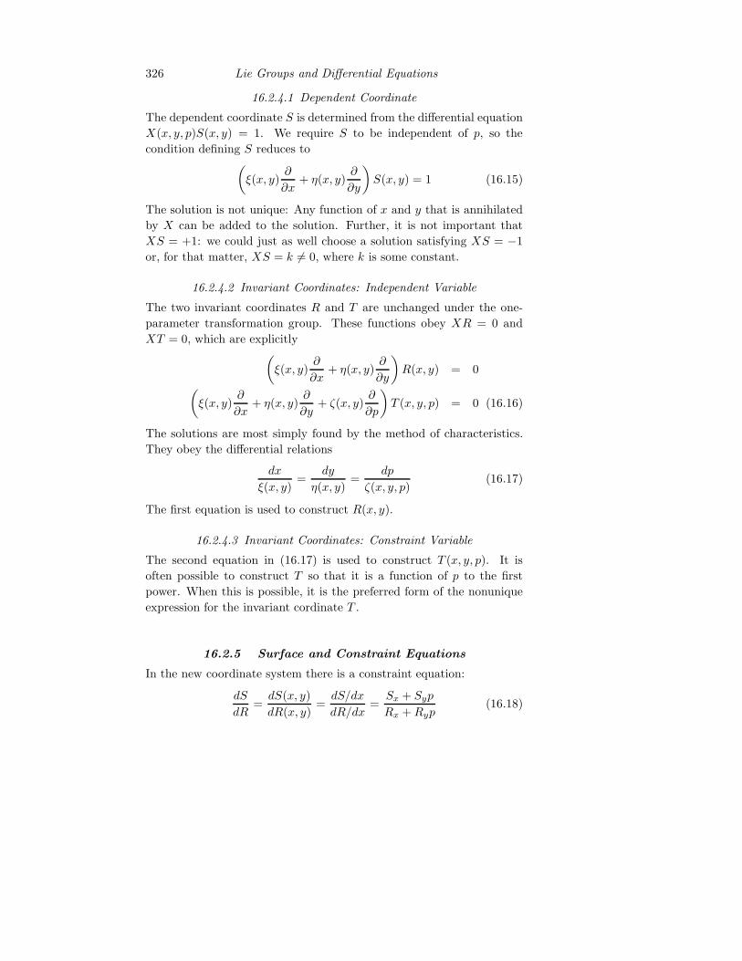
The surface p = y2− y/x is shown in Fig. 16.1. The value of p clearly
depends on both coordinates x and y. The purpose of the change of
variables to to find a new coordinate system in which the surface is
independent of the new dependent variable S(x, y).
Fig. 16.1. The first order ODE xp + y − xy2 = 0. Here p (vertical) is plottedover the (x, y) plane for 0.1 ≤ x ≤ 1.1 and −2 ≤ y ≤ +2. The shape of thesurface depends on both coordinates x and y.
The determining equation Eq. (16.14) is
ξ(p− y2) + η(1− 2xy) +[
ηx + (ηy − ξx)p− ξyp2]
x = 0 (16.22)
The functions ξ(x, y) and η(x, y) describing the generators of infinites-
imal displacements are determined following the algorithm outlined in
Sect. 16.2.3. First, we use the surface equation F (x, y, p) = 0 to find
an expression for p: p(x, y) = −y/x + y2. This is substituted into the
determining equation XF (x, y, p) = 0 to provide a functional relation
16.3 An Example 329
between x and y:
ξ(
− yx
)
+η(1−2xy)+ηxx+(ηy−ξx)(xy2−y)−ξy(
xy4 − 2y3 +y2
x
)
= 0
(16.23)
We first attempt zeroth degree expressions for ξ and η: ξ = ξ00, η = η00.
When these are substituted into Eq. (16.23) we obtain three equations
for the two unknowns. The coefficients of the monomials y/x, 1, and xy
depend on the unknown parameters ξ00, η00 as follows:
Monomial ξ00 η00y/x
x0y0 = 1
xy
−1 0
0 1
0 −2
[
ξ00η00
]
=
[
0
0
]
(16.24)
This system of three simultaneous linear equations in two unknowns has
rank two, therefore no nontrivial solutions.
We therefore increase the degree of ξ(x, y) and η(x, y) to one and
repeat the process. The relation Eq. (16.23) between x and y is now
(ξ00 + ξ10x+ ξ01y)(
− yx
)
+ (η00 + η10x+ η01y)(1− 2xy) + η10x+
(η01 − ξ10)(xy2 − y)− ξ01(
xy4 − 2y3 +y2
x
)
= 0 (16.25)
This results in the following set of 10 equations for 6 unknowns:
Monomial ξ00 ξ10 ξ01 η00 η10 η01y2/x
y/x
1
x
y
xy
x2y
xy2
xy3
xy4
0 0 −2 0 0 0
−1 0 0 0 0 0
0 0 0 +1 0 0
0 0 0 0 +2 0
0 0 0 0 0 0
0 0 0 −2 0 0
0 0 0 0 −2 0
0 −1 0 0 0 −1
0 0 −2 0 0 0
0 0 +1 0 0 0
ξ00ξ10ξ01η00η10η01
=
0
0
0
0
0
(16.26)
This set of equations has rank 5, so there is one nontrivial solution. From
the first four equations we determine ξ01 = ξ00 = η00 = η10 = 0, and
from the coefficient of xy2 we learn −ξ10 − η01 = 0 so that, up to some
overall scaling factor we can take ξ(x, y) = x and η(x, y) = −y. Since
330 Lie Groups and Differential Equations
we have found one nontrivial solution for an infinitesimal generator of
a one-parameter group of a first order equation, we can stop searching
for additional solutions to the determining equation (for second order
equations there may be additional solutions).
With this solution ξ(x, y) = x and η(x, y) = −y the prolongation
formula Eq. (16.8) gives ζ = −2p, so that the generator of infinitesimal
displacements is
X = x∂
∂x− y ∂
∂y− 2p
∂
∂p(16.27)
The infinitesimal generator is now used to determine the new set of
coordinates. We first determine the dependent coordinate S(x, y) by
attempting to solve(
x∂
∂x− y ∂
∂y
)
S(x, y) = 1 (16.28)
It is useful first to seek a solution S(x, y) depending only on the single
variable y. Such a solution can be found if the equation −ydS(y)/dy = 1
can be solved. The solution, up to an additive constant, is − ln(y). We
will adopt this solution, neglecting the negative sign: S(x, y) = ln(y).
The invariant coordinates are determined using the method of char-
acteristics:dx
x=
dy
−y =dp
−2p(16.29)
The first equation for the new independent variable simplifies to ydx =
−xdy or d(xy) = 0, from which we conclude that R(x, y) = xy is an
invariant coordinate that obeys Eq. (16.14). The invariant coordinate
involving p is determined by setting −dp/2p equal to either of the other
two differentials. We set it equal to dx/x to avoid having the second in-
variant coordinate dependent on y. The equation is dx/x = −dp/2p and
the solution is (1/x)d(x2p) = 0, so that T (x, y, p) = x2p. The forward
and backward transformations between the two coordinate systems are
R
S
T
=
xy
ln(y)
x2p
x
y
p
=
Re−S
eS
Te2S/R2
(16.30)
In the new coordinate system the surface equation transforms to
F (x, y, p) = xp+ y − xy2 = 0 −→ eS
[
T
R+ 1−R
]
= 0 (16.31)
The expression within the bracket is the transformed surface equation.
16.3 An Example 331
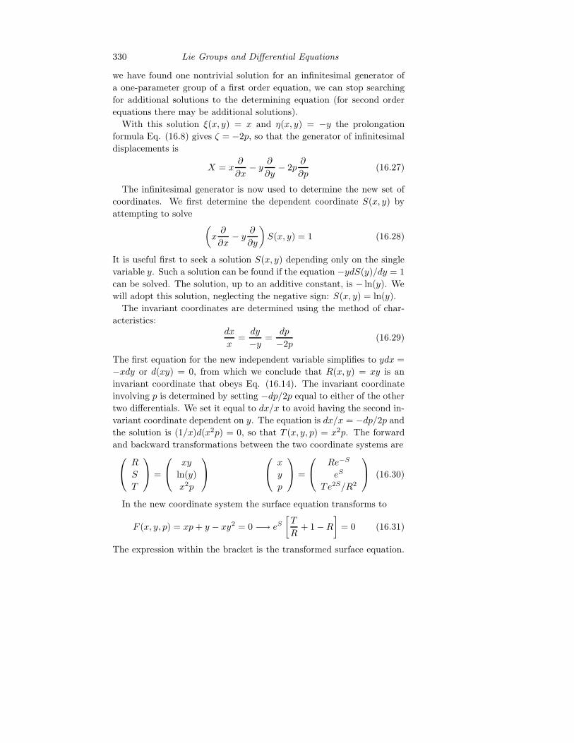
It is independent of S. This surface T = T (R,S) is plotted in Fig.
16.2. It has the desired form: a ruled surface whose shape (height) is
independent of the dependent variable S. Such a surface is sometimes
called a “cylinder.”
Fig. 16.2. The surface xp+y−xy2 = 0 transforms to the surface T/R+1−R =0 in canonical coordinates. Here T (vertical) is plotted over the (R, S) planefor −3 ≤ R ≤ +4 and −2 ≤ S ≤ +2. The function is a simple ruled surface,independent of S.
The new constraint equation is
dS
dR=d(ln y)
d(xy)=
p/y
y + xp=
TeS/R2
eS + (Re−S)(Te2S/R2)(16.32)
The surface and constraint equations are
Surface equation : T/R+ 1−R = 0
Constraint equation : dS/dR = (T/R)/(T +R)(16.33)
The surface equation is solved for T as a function ofR: T (R) = R2−R.
This expression is substituted into the constraint equation to give a first
332 Lie Groups and Differential Equations
order differential equation in quadratures:
dS
dR=
1
R− 1
R2=⇒ S = ln(R) +
1
R+ c (16.34)
The parameter c is the parameter of the translation group that leaves
invariant the transformed equation.
The inverse transformation, Eq. (16.30), from (R,S) to (x, y) is finally
used to rewrite the solution in terms of the original set of variables:
y =−1
x(c+ lnx)(16.35)
Remarks: The operator x ddx is the infinitesimal generator for scal-
ing transformations, since eλx ddxx = eλx. As a result, the infinitesimal
generator X has the following effect on the coordinates (x, y, p):
EXP
(
λ
{
x∂
∂x− y ∂
∂y− 2p
∂
∂p
})
x
y
p
=
eλx
e−λy
e−2λp
(16.36)
From this scaling behavior, it is easy to see that ln(y) is linear in the
Lie translation group parameter: ln(e−λy) = ln(y) − λ. The invariant
operators come right out of the scaling transformations: xy and x2p are
unchanged by the scaling transformation. None of these operators is
unique. The operator ln(xy2) is linear and x3yp is invariant. We have
just chosen the most convenient (simplest) solutions to the equations
defining the new coordinates.
16.4 Additional Insights
Lie’s theory of infinitesimal transformation groups has been extended
in many different directions, all of which are powerful and beautiful. It
is barely possible to scratch the surface here. Instead, we content our-
selves by indicating some of the directions in which it can be extended.
These directions are simple consequences of the analyses presented in
the previous two sections.
16.4.1 Other Equations, Same Symmetry
Many differential equations can share the same invariance group. The
most general first order ordinary differential equation invariant under the
scaling group Eq. (16.36) has the form F (R,−, T ) = 0 or more simply
F (xy, x2p) = 0. The most general first order equation of first degree
16.4 Additional Insights 333
with this symmetry has the form x2p = h(xy) or dy/dx = x−2h(xy).
For the equation studied in Sect. 16.3, h(z) = −z + z2. For the Riccati
equation dy/dx+ y2 − 2/x2 = 0, h(z) = z2 − 2.
16.4.2 Higher Degree Equations
These methods work equally well with first order equations of higher
degree. For example, the first order, second degree equation y′2 + y4 −x−4 = 0 has canonical form R4 +T 2 = 1. The original equation has two
solution branches p = ±√
x−4 − y4, corresponding to the two solution
branches in the canonical coordinate system T = ±√
1−R4.
16.4.3 Other Symmetries
The methods described in Sect. 16.2 and illustrated by example in Sect.
16.3 apply to any first order ordinary differential equation with a one
parameter group. Table 16.1 provides a list of symmetries that may be
encountered for ordinary differential equations. For each symmetry the
functions ξ(x, y) and η(x, y) are tabulated, as well as the first prolonga-
tion ζ(x, y, p) = η(1)(x, y, p). We also present the canonical coordinates
(R,S, T ). Since the constraint equation dS/dR depends only on the
change of variables, it also can be tabulated, and has been. The sim-
plest case, Eq. (16.1), is present in the first line of this table. The
equation studied in Sect. 16.3 is present in the eighth line of this table.
The Lie symmetries leaving the equation invariant can be determined
from this table in one of two ways. We can use the generator of in-
finitesimal displacements to compute them, as in Eq. (16.36). Or we
can look at the transformations effected by S → S′ = S + c, R′ = R. In
the latter case we find ln(y)→ ln(y) + c = ln(ecy) = ln(y(c)) and since
xy = x(c)y(c), the transformation is x(c) = e−cx and y(c) = e+cy.
16.4.4 Second Order Equations
Second order equations can be studied by simple extensions of the meth-
ods used to study first order equations. The infinitesimal generator for
displacements now involves derivatives with respect to y(2) and is given
by
X = ξ∂
∂x+ η
∂
∂y+ η(1) ∂
∂y(1)+ η(2) ∂
∂y(2)(16.37)
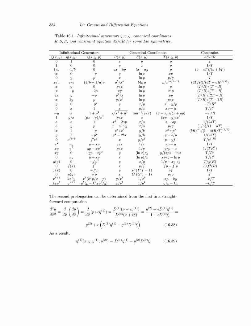
334 Lie Groups and Differential Equations
Table 16.1. Infinitesimal generators ξ, η, ζ, canonical coordinates
R,S, T , and constraint equation dS/dR for some Lie symmetries.
Infinitesimal Generators Canonical Coordinates Constraintξ(x, y) η(x, y) ζ(x, y, p) R(x, y) S(x, y) T (x, y, p) dS/dR
0 1 0 x y p T1 0 0 y x p 1/T
1/a −1/b 0 ax + by bx − ay p (b − aT )/(a + bT )x 0 −p y ln x xp 1/T0 y p x ln y p/y T
x/a y/b (1/b − 1/a)p yb/xa b ln y p/x(a/b−1) (bT/R)/(bT − aR(1/b))x y 0 y/x ln y p (T/R)/(T − R)x −y −2p xy ln y x2p (T/R)/(T + R)2x y −p y2/x ln y yp (T/R)/(2T − R)x 2y p y/x2 ln y p/x (T/R)/(T − 2R)y 0 −p2 y x/y x − y/p −T/R2
0 x 1 x y/x xp − y T/R2
−y x 1 + p2p
x2 + y2 tan−1(y/x) (y − xp)/(x + yp) −T/R1 y/x (px − y)/x2 y/x x (xp − y)/x2 1/Ta x 1 x2
− 2ay x/a x − ap 1/(2aT )a y p x − a ln y x/a p/y (1/a)/(1 − aT )
x b −p ey/xb y/b ey∗ pb (bR)−1/[1 − b(R/T )(1/b)]
y b −p2 y2− 2bx y/b y − b/p 1/(2bT )
0 ef(x) f ′ef x y/ef p − yf ′ T/ef(R)
x2 xy y − xp y/x 1/x xp − y 1/Txy y2 yp − xp2 y/x 1/y y/p − x 1/(TR2)xy 0 −yp− xp2 y (ln x)/y y/(xp) − lnx T/R2
0 xy y + xp x (ln y)/x xp/y − ln y T/R2
g(y) 0 −g′p2 y x/g 1/p − xg′/g T/g(R)0 f(x) f ′ x y/f fp − f ′y T/f2(R)
f(x) 0 −f ′p y F (F ′f = 1) pf 1/T0 g(y) g′p x G (G′g = 1) p/g T
xk+1 kxky xk(k2y/x − p) y/xk 1/xk xp − ky −k/Tkxyk yk+1 yk(p − k2xp2/y) x/yk 1/yk y/p − kx −k/T
The second prolongation can be determined from the first in a straight-
forward computation
d2y
dx2=
d
dx
(
dy
dx
)
=d
dx(p+ǫη(1)) =
D(1)(p+ ǫη(1))
D(0)(x+ ǫξ)=y(2) + ǫD(1)η(1)
1 + ǫD(0)ξ=
y(2) + ǫ(
D(1)η(1) − y(2)D(0)ξ)
(16.38)
As a result,
η(2)(x, y, y(1), y(2)) = D(1)η(1) − y(2)D(0)ξ (16.39)
16.4 Additional Insights 335
where
D(n) =∂
∂x+dy
dx
∂
∂y+dy(1)
dx
∂
∂y(1)+ · · ·+ y(n+1) ∂
∂y(n)(16.40)
It is explicitly
η(2) = ηxx+(2ηxy−ξxx)y′+(ηyy−2ξxy)y′2−ξyyy
′3+(ηy−2ξx−3ξyy′)y′′
(16.41)
The determining equations are
F (x, y, y(1), y(2)) = 0 X(x, y, y(1), y(2))F (x, y, y(1), y(2)) = 0
(16.42)
Symmetries are found by following the algorithm described in Sect.
16.2.3 and illustrated in Sect. 16.3.
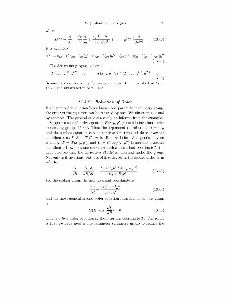
16.4.5 Reduction of Order
If a higher order equation has a known one-parameter symmetry group,
the order of the equation can be reduced by one. We illustrate as usual
by example. The general case can easily be inferred from the example.
Suppose a second order equation F (x, y, y′, y′′) = 0 is invariant under
the scaling group (16.36). Then the dependent coordinate is S = ln y
and the surface equation can be expressed in terms of three invariant
coordinates as F (R,−, T, U) = 0. Here as before R depends only on
x and y, T = T (x, y, y′), and U = U(x, y, y′, y′′) is another invariant
coordinate. How does one construct such an invariant coordinate? It is
simple to see that the derivative dT/dR is invariant under the group.
Not only is it invariant, but it is of first degree in the second order term
y(2), for
dT
dR=dT/dx
dR/dx=Tx + Tyy
(1) + Ty(1)y(2)
Rx + Ryy(1)(16.43)
For the scaling group the new invariant coordinate is
dT
dR=
2xy′ + x2y′′
y + xy′(16.44)
and the most general second order equation invariant under this group
is
G(R,−, T, dTdR
) = 0 (16.45)
This is a first order equation in the invariant coordinate T . The result
is that we have used a one-parameter symmetry group to reduce the
336 Lie Groups and Differential Equations
order of a second order equation by one. If an additional symmetry can
be identified, the equation can be reduced to quadratures a second time
(i.e., completely integrated).
The most general second order equation invariant under the group of
scaling transformations Eq. (16.36) that is of first degree in y′′ is
dT
dR=x2y′′ + 2xy′
y + xy′= g(xy, x2y′) = g(R, T ) (16.46)
This is a first order equation in T . Certain forms of the function g may
admit another Lie symmetry. If such a symmetry can be found, the
order of the equation can again be reduced by one.
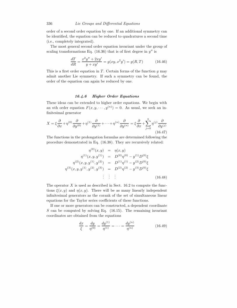
16.4.6 Higher Order Equations
These ideas can be extended to higher order equations. We begin with
an nth order equation F (x, y, · · · , y(n)) = 0. As usual, we seek an in-
finitesimal generator
X = ξ∂
∂x+η(0) ∂
∂y(0)+η(1) ∂
∂y(1)+ · · ·+η(n) ∂
∂y(n)= ξ
∂
∂x+
n∑
j=0
η(j) ∂
∂y(j)
(16.47)
The functions in the prolongation formulas are determined following the
procedure demonstrated in Eq. (16.38). They are recursively related:
η(0)(x, y) = η(x, y)
η(1)(x, y, y(1)) = D(0)η(0) − y(1)D(0)ξ
η(2)(x, y, y(1), y(2)) = D(1)η(1) − y(2)D(0)ξ
η(3)(x, y, y(1), y(2), y(3)) = D(2)η(2) − y(3)D(0)ξ
......
... (16.48)
The operator X is used as described in Sect. 16.2 to compute the func-
tions ξ(x, y) and η(x, y). There will be as many linearly independent
infinitesimal generators as the corank of the set of simultaneous linear
equations for the Taylor series coefficients of these functions.
If one or more generators can be constructed, a dependent coordinate
S can be computed by solving Eq. (16.15). The remaining invariant
coordinates are obtained from the equations
dx
ξ=
dy
η(0)=dy(1)
η(1)= · · · = dy(n)
η(n)(16.49)
16.4 Additional Insights 337
In fact, only the first two invariant coordinates R(x, y) and T (x, y, y(1))
need be computed. The remaining invariant coordinates are dT (j)/dR(j),
j = 0 (for T ) and j = 1, 2, · · · , n−1. Each of these latter is of first degree
in y(j+1). As a result, the existence of a Lie symmetry can be used to
reduce an nth order equation to an (n− 1)st order equation.
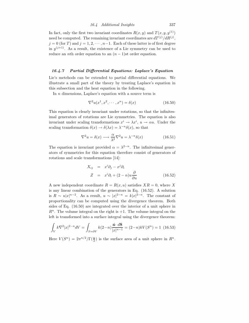
16.4.7 Partial Differential Equations: Laplace’s Equation
Lie’s metehods can be extended to partial differential equations. We
illustrate a small part of the theory by treating Laplace’s equation in
this subsection and the heat equation in the following.
In n dimensions, Laplace’s equation with a source term is
∇2u(x1, x2, · · · , xn) = δ(x) (16.50)
This equation is clearly invariant under rotations, so that the infinites-
imal generators of rotations are Lie symmetries. The equation is also
invariant under scaling transformations xi → λxi, u → αu. Under the
scaling transformation δ(x)→ δ(λx) = λ−nδ(x), so that
∇2u = δ(x) −→ α
λ2∇2u = λ−nδ(x) (16.51)
The equation is invariant provided α = λ2−n. The infinitesimal gener-
ators of symmetries for this equation therefore consist of generators of
rotations and scale transformations [14]:
Xij = xi∂j − xj∂i
Z = xi∂i + (2− n)u∂
∂u(16.52)
A new independent coordinate R = R(x, u) satisfies XR = 0, where X
is any linear combination of the generators in Eq. (16.52). A solution
is R ∼ u|x|n−2. As a result, u ∼ |x|2−n = k|x|2−n. The constant of
proportionality can be computed using the divergence theorem. Both
sides of Eq. (16.50) are integrated over the interior of a unit sphere in
Rn. The volume integral on the right is +1. The volume integral on the
left is transformed into a surface integral using the divergence theorem:∫
V
k∇2|x|2−ndV =
∫
S=∂V
k(2−n)n· dS|x|n−1
= (2−n)kV (Sn) = 1 (16.53)
Here V (Sn) = 2πn/2/Γ(n2 ) is the surface area of a unit sphere in Rn.
338 Lie Groups and Differential Equations
As a result, the solution of Laplace’s equation in Rn (n 6= 2) with unit
source term at the origin is
u(x) =k
|x|n−2k =
−1
(n− 2)V (Sn)(16.54)
16.4.8 Partial Differential Equations: Heat Equation
The heat equation on Rn for u(x, t) with source term
ut −∇2u = δ(x, t) (16.55)
is treated similarly [55]. It is invariant under rotations, so the operators
Xij are Lie symmetries. Under the scaling transformation u → αu,
t→ βt, and xi → λxi the equation transforms as follows:
ut −∇2u = δ(x, t) −→ α
βut −
α
λ2∇2u =
1
λnβδ(x, t) (16.56)
Invariance under the scaling transformations places the following two
constraints on the three scaling variables (since there is only one equa-
tion): αλn = 1 and β/λ2 = 1. From these relations it is possible to
construct n+ 1 additional Lie symmetries, so that the entire set is
Xij = xi∂j − xj∂i
Yi = 2t∂
∂xi− xiu
∂
∂u(16.57)
Z = 2t∂
∂t+ xi ∂
∂xi− nu ∂
∂u
An invariant coordinate depending on the xi, t and u is R = utn/2e|x|2/4t,
from which we obtain as before
u = kt−n/2e−|x|2/4t k =
(
1
2√π
)n
(16.58)
16.4.9 Closing Remarks
Galois resolved the problem of determining if an algebraic equation
could be solved by radicals, and if so how, between 1829 and 1832.
His manuscripts were lost, rejected, or filed for posterity. His accom-
plishments were unrecognized at his death in 1832. They were rescued
from oblivion, the black hole of French indifference to its greatest math-
ematician, by Cauchy in 1843.
Lie’s discoveries began in 1874. He realized that the hodgepodge of
16.5 Conclusion 339
seemingly different techniques for solving differential equations that ex-
isted at that time (and still does) were almost all special manifestations
of one single principle — the invariance of solutions of ordinary differ-
ential equations under a continuous group. Lie was luckier than Galois
when it came to recognition during his lifetime.
There are several problems in the implementation of Lie’s algorithms
that have either been lightly addressed or passed over in our discussion.
These are:
(i) Under what conditions is it possible to solve the determining
equations for the surface? That is, when is it possible — or
impossible — to solve the linear partial differential equations for
ξ(x, y) and η(x, y)?
(ii) Under what conditions is it possible to solve the determining
equations for the canonical variables?
(iii) Under what conditions is it possible to solve the canonical surface
equation F (R,−, T ) = 0 for T as a function of R? When it is
possible, what is the algorithm for accomplishing this?
(iv) Under what conditions is it possible to integrate a function of a
single variable:∫
f(R,-, T (R))dR?
The final question has been resolved for algebraic functions by Risch in
1969 [58]. He exploited the tools of Galois theory in a heavy way to
provide an algorithm for determining when an algebraic function can
be integrated in closed form, and determining the integral when the
answer to the first question is positive. We summarize the dates of these
accomplishments here
1830 Galois Solve algebraic equations.
1874 Lie Solve differential equations.
1969 Risch Integrate in closed form.
? — Solve determining equations for ξ, η.
? — Solve determining equations for R,S, T .
? — Solve F (R,−, T ) = 0 for R.
It is clear that additional algorithms are possible and desirable.
16.5 Conclusion
Lie set out to extend Galois’ treatment of algebraic equations to the
field of ordinary differential equations. Galois observed that an alge-
braic equation has a symmetry group: a set of operations that maps
340 Lie Groups and Differential Equations
solutions into solutions. If the symmetry group has certain properties,
these properties can be used to generate an algorithm for solving the
equation.
It was Lie’s genius to see that the “trivial” additive constant that oc-
curs in the solution of a differential equation that has been reduced to
quadratures is in fact a group operation. The symmetry group in this
simplest case is simply the one parameter group of translations. Armed
with this observation, he developed algorithmic methods to attack ordi-
nary differential equations by searching for their symmetry groups. Lie
in fact studied local groups of transformations. The even more beautiful
study of global Lie groups was a later development.
In Sect. 16.2 we presented Lie’s algorithm for solving first order ordi-
nary differential equations in a number of simple steps. These involve:
(i) Introduce a set of point transformations in the x-y plane. These
are defined by the functions ξ(x, y) and η(x, y).
(ii) Construct the first prolongation ζ(x, y, p) = η(1)(x, y, y(1)) from
the functions defining the local change of variables.
(iii) Introduce the operator X = ξ ∂∂x + η ∂
∂y + ζ ∂∂p . This describes
a Taylor series expansion of the surface equation F (x, y, p) = 0
that defines the first order ODE.
(iv) Solve the determining equation XF = 0 when F = 0 for the
functions ξ(x, y) and η(x, y).
(v) Solve the determining equations XR = 0, XS = 1, XT = 0 for
the canonical coordinates. These are the coordinates in which
the surface is a “cylinder:” The surface equation is independent
of the new dependent variable: F → F (R,−, T ) = 0.
(vi) Construct the constraint equation dS/dR = f(R,−, T ) in this
new coordinate system.
(vii) Solve the surface equation for T as a function of R: T = T (R).
(viii) Solve the constraint equation for S: S =∫
f(R,−, T (R)) + c.
(ix) Backsubstitute the original coordinates for the new coordinates:
x = x(R,S) and y = y(R,S) to obtain the solution of the original
equation.
The steps in this algorithm have been illustrated by working out a simple
example in Sect. 16.3.
These methods extend in any number of ways. We have indicated a
number of useful directions by example in Sect. 16.4.
16.6 Problems 341
16.6 Problems
1. Show that invariance under a one-parameter group of transformations
can also be expressed in the form
dn
dǫnF [x(ǫ), y(ǫ), p(ǫ)]|ǫ=0 = 0, n = 0, 1, 2, · · · (16.59)
Show that the first two terms n = 0, 1 are exactly the determining
equations 16.12.
2. Construct the invariance group for each of the transformations
presented in Table 16.1.
3. Mechanical Similarity: The classical newtonian equation of
motion for a particle of mass m in the presence of a potential V (x) is
md2x
dt2= −∇V (x)
Assume that under a scaling transformation, the mass scales with a
factor α (i.e., m → αm), x → βx, t → γt. Assume also that the
potential is homogeneous of degree k: V (βx) → βkV (x) [49]. Under
this scaling transformation show that the equation of motion transforms
to
α1β1γ−2md2x
dt2= −βk−1∇V (x)
a. Show that the scaled equation is identical to the original provided
α1β2−k γ−2 = 1.
b. Set α = 1. Show that trajectories are invariant under the scaling
transformation with γ2 = β2−k. Show that in the cases k = −1, k =
0, k,= +1, k = +2 the following scaling results hold:
k Potential Type transformation
−1 Coulomb γ2 = β3
0 No Force γ2 = β2
+1 Local Gravitational Potential γ2 = β1
+2 Harmonic Oscillator γ2 = β0
The first line is a statement of Kepler’s Third Law: for closed planetary
orbits, the square of the period (γ2) is proportional to the cube of the
semiaxis (β3). If R′ and T ′ are the semiaxis and period of planet P ′ and
R and T are the semiaxis and period of planet P , and the two planets
342 Lie Groups and Differential Equations
P and P ′ have geometrically similar orbits, β3 → (R′/R)3 = (T ′/T )2 ←γ2. The second line is a statement of the integral of Newton’s second
law in the absence of forces in an inertial frame: the distance traveled
(β) is proportional to the time elapsed (γ). The third line is a statement
that in a local gravitational potential of the form V = mgz, the distance
fallen increases like the square of the time elapsed. The fourth line
is a statement of Hooke’s Law: in harmonic motion the period (γ) is
independent of the size of the orbit.
c. Fix γ = 1 and construct a table relating the mass and orbital scale
under the four forces described in the table above.
d. Fix β = 1 and show that the period scales like√M for all homoge-
neous potentials. Reconcile this result with the well-known result that
the period of a planet is independent of its mass in lowest order.
e. If the motion is bounded for all times, show
2〈T 〉 = 〈x·∇V (x)〉 = 〈kV (x)〉
where T is the kinetic energy. This is the Virial Theorem for homoge-
noeous potentials.
f. Show that the kinetic energy scales like αβ2γ−2 = βk (use a.).
Since the potential energy scales the same way, the total energy has this
scaling property.
4. Assume that the dynamics of a system are derivable from an action
principle: for example, the Euler-Lagrange equations are derived from
the variation of an action: δ∫
L(x, x)dx = 0. Show that if a scaling
transsformation leaves the Lagrangian invariant up to an overall scaling
factor, the trajectories will scale under this transformation.
5. The heat equation in one dimension is
∂2u
∂x2=∂u
∂t
Show that the following six differential operators vi are infinitesimal
generators of the invariance group of this equation. Show that eǫvif(x, t)
has the action shown for each of the six generators [55]:
16.6 Problems 343
vi Infinitesial eǫvif(x, t) =
v1 ∂x f(x− ǫ, t)v2 ∂t f(x, t− ǫ)v3 u∂u eǫf(x, t)
v4 x∂x + 2t∂t f(e−ǫx, e−2ǫt)
v5 2t∂x − xu∂u e−ǫx+ǫ2tf(x− 2ǫt, t)
v6 4xt∂x + 4t2∂t − (x2 + 2t)u∂u λe−ǫλ2x2
f(λ2x, λ2t)
where λ2 = 1/(1 + 4ǫt)
6. The two dimensional wave equation is
∂2u
∂x2+∂2u
∂y2=∂2u
∂t2
Show that the following vector fields map solutions into solutions:
Displacements Pi ∂x, ∂y, ∂t
Rotations Lz x∂y − y∂x
Boosts Bi x∂t + t∂x, y∂t + t∂y
Dilations Di x∂x + y∂y + t∂t, u∂u
Inversions
ixiyit
=
x2 − y2 + t2 2xy 2xt −xu2yx −x2 + y2 + t2 2yt −yu2tx 2ty x2 + y2 + t2 −tu
∂x
∂y
∂t
∂u
Show thatD2 = u∂u commutes with all remaining generators. Construct
the commutation relations of the remaining ten generators, and show
they satisfy the commutation relations of the conformal group in 2+1
dimensions. Show that this group is SO(2 + 1, 1 + 1) = SO(3, 2).
7. Construct the invariance group for the wave equation in 3+1 di-
mensions. This is the Maxwell equation without sources in space time.
There are 16 infinitesimal generators. Show that 15 satisfy the commu-
tation relations for the conformal group SO(3 + 1, 1 + 1) = SO(4, 2) [9].
The extra generator commutes with all the rest, and is u∂u.
8. The heat equation in one dimension is uxx−ut = 0. The infinitesi-
mal generator of symmetries for this equation is X = ξi ∂∂xi +η ∂
∂u + · · · =ξ1 ∂
∂x + ξ2 ∂∂t + η ∂
∂u + · · · . Show that [66]
344 Lie Groups and Differential Equations
ξ1 = a1 + a2x+ a3t+ a4xt
ξ2 = 2a2t+ a4t2 + a5
η = − 12a3xu− a4(
12 t+
14x
2)u+ a6u+ h(x, t)
Here h(x, t) is any function that satisfies the homogeneous heat equation.
Construct the infinitesimal generators corresponding to the arbitrary
real coordinates ai and compute their commutation relations. What is
the structure of this Lie algebra?
9. Show that the scalar operator
S = t2∂
∂t+ tx · ∇ − 1
4(x · x + 2nt) u
∂
∂u
is also a Lie symmetry of Eq. (16.55) with source term.
10. Noether’s Theorem for Physicists: Many dynamical prob-
lems can be expressed in an action principle format:
I =
∫ t2
t1
L(t, x, x)dt, δI = 0
Specifically, the action I is stationary on a physically allowed trajectory.
The first variation leads to the Euler-Lagrange equations
d
dt
(
∂L
∂xi
)
− ∂L
∂xi= 0
Under a one parameter family of change of variables: t→ t′ = T (t, x, ǫ) =
t+ǫξ(t, x), xi → x′i = Xi(t, x, ǫ) = xi+ǫηi(t, x) the action integral trans-
forms to
I =
∫ t′
2
t′
1
L(t′, x′, x′)dt′ =
∫ t2
t1
L(t′, x′, x′)dt′
dtdt
where dt′/dt = ∂T/∂t+ (∂T/∂xi)dxi/dt. Show that if you differentiate
the action integral with respect to ǫ, then set ǫ = 0 the result is
∫ t2
t1
(
ξ∂L
∂t+ ηi
∂L
∂xi+ η
(1)i
∂L
∂xi+dξ
dtL
)
dt = 0
Show that by standard arguments the integrand must itself be zero.
Show that along an allowed trajectory the vanishing of the integrand
can be expressed in the form
16.6 Problems 345
d
dt[ξL+ (ηi − ξxi)Lxi
] = 0
The expression within the square brackets is a constant of the motion.
Apply this theorem to a Lagrangian that is invariant under space dis-
placements, time displacements, and rotations around a space axis to
construct the following conserved quantities:Symmetry Conserved Quantity
Space Displacements Momentum
Time Displacements Energy
Space-Time Displacements Four-Momentum
Rotations Angular Momentum
11. Noether’s Theorem, More General: We present a more gen-
eral form of Noether’s theorem than is presented above. This form is
very powerful and sufficient for most physical applications. It is not the
most general form of Noether’s theorem. Suppose the dynamics of a sys-
tem is derivable from an action integral of the form L[u] =∫
L(x, u)dx,
x ∈ Rp, u ∈ Rq, and suppose the infinitesimal generators that leave the
dynamics invariant has the from
v =
p∑
i=1
ξi(x, u)∂
∂xi+
q∑
α=1
φα(x, u)∂
∂uα
Show that the components Pi defined by
P i = ξiL+
q∑
α=1
φα(x, u)∂L∂uα
i
−q
∑
α=1
p∑
j=1
ξjuαj
∂L∂uα
i
satisfy a conservation law of the form
∇P = div P =∂P i
∂xi= 0
12. Representation Theory: G is a compact Lie group with in-
variant measure dρ(g) and volume V ol(G) =∫
dρ(g), Γλµν(g) are the ir-
reducible representations of G constructed by reduction of tensor prod-
ucts (Wigner-Stone theorem), and φ(g), ψ(g) are functions defined on
the group manifold. The orthogonality and completeness relations are
∫
dim λ
V ol(G)Γλ′∗
µ′ν′(g)Γλµν(g)dρ(g) = δλ′λδµ′µδν′ν
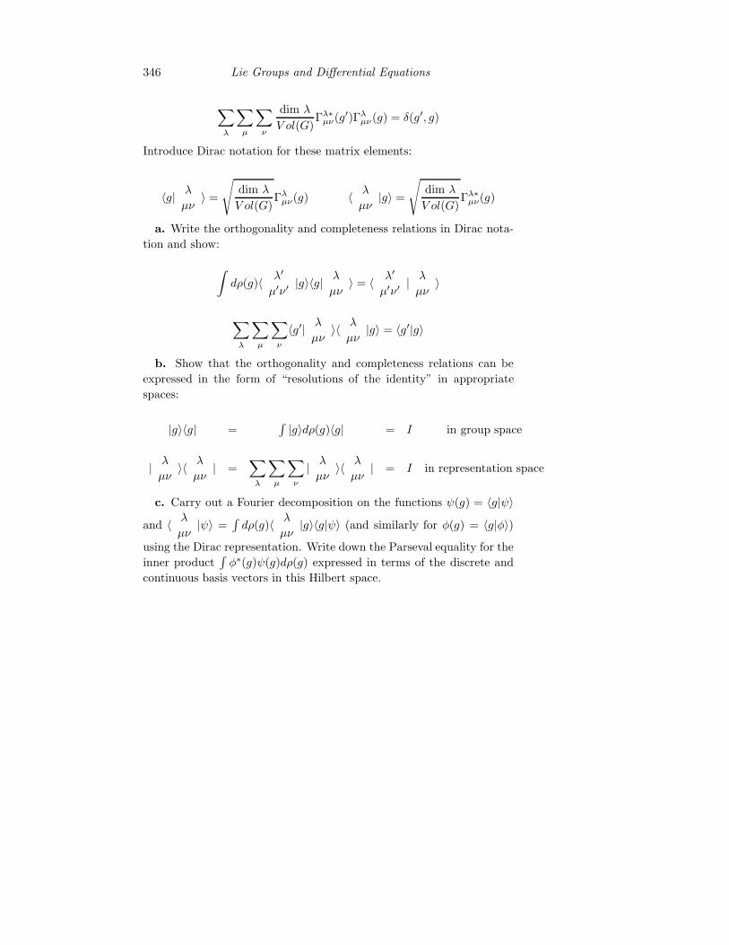
346 Lie Groups and Differential Equations
∑
λ
∑
µ
∑
ν
dim λ
V ol(G)Γλ∗
µν(g′)Γλµν(g) = δ(g′, g)
Introduce Dirac notation for these matrix elements:
〈g| λµν〉 =
√
dim λ
V ol(G)Γλ
µν(g) 〈 λ
µν|g〉 =
√
dim λ
V ol(G)Γλ∗
µν(g)
a. Write the orthogonality and completeness relations in Dirac nota-
tion and show:
∫
dρ(g)〈 λ′
µ′ν′|g〉〈g| λ
µν〉 = 〈 λ′
µ′ν′| λµν〉
∑
λ
∑
µ
∑
ν
〈g′| λµν〉〈 λ
µν|g〉 = 〈g′|g〉
b. Show that the orthogonality and completeness relations can be
expressed in the form of “resolutions of the identity” in appropriate
spaces:
|g〉〈g| =∫
|g〉dρ(g)〈g| = I in group space
| λ
µν〉〈 λ
µν| =
∑
λ
∑
µ
∑
ν
| λ
µν〉〈 λ
µν| = I in representation space
c. Carry out a Fourier decomposition on the functions ψ(g) = 〈g|ψ〉
and 〈 λ
µν|ψ〉 =
∫
dρ(g)〈 λ
µν|g〉〈g|ψ〉 (and similarly for φ(g) = 〈g|φ〉)
using the Dirac representation. Write down the Parseval equality for the
inner product∫
φ∗(g)ψ(g)dρ(g) expressed in terms of the discrete and
continuous basis vectors in this Hilbert space.


![Superposition rules, Lie theorem, and partial differential ... · Superposition rules, Lie theorem, and partial differential equations ... [15] he was able to ... superposition](https://img.pdfslide.net/doc/110x75/5b51ae327f8b9a7b648c4dfc/superposition-rules-lie-theorem-and-partial-dierential-superposition.jpg)