• an earlier class covered the unique one-dimensional well-mixed LS model for Gaussian inhomogeneous turbulence (used in assig. 3)

• today a quick look at a well-mixed two-dimensional LS model for horizontally-homogeneous Gaussian turbulence

• then a look at the corresponding three-dimensional LS model for fully-inhomogeneous Gaussian turbulence

16 Nov., 2010

eas572_urbanLS.pptJDW, 16 Nov. 2010

Eulerian approach:“Mass is conserved...”

Lagrangian:“Track motion...”

∂∂

∂∂

∂∂

∂∂

∂∂

ct

ucx

wcz x

u cz

w c+ + = − −' ' ' 'Z t dt Z t W dtW t dt W t dWdW a dt b d

( ) ( )( ) ( )

( , )

+ = ++ = += +X U ξ

“... during advection and ‘diffusion’ between control volumes... ”

memorymemory randomrandomforcingforcing

t+dtt+dt

tt

w c KCz

' ' = −∂∂

+ closure

ii--1, j1, j--11

i+1, j+1i+1, j+1

i , ji , j

Thomson’s well-mixed LS model for 2-D Gaussian, vertically-inhomogeneous turbulence

where ; ; is the Eulerian joint

PDF for u, w (specifically, the joint Gaussian); and:

The well-mixed condition is a single equation constraining the vector coefficient ai =(au , aw ) of the generalized Langevin equation, and (in the case of multi-dimensional models) selects a class of models – but not a unique model.

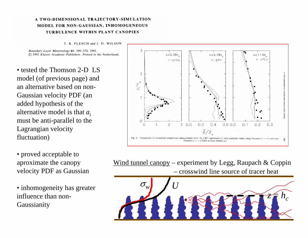
• tested the Thomson 2-D LS model (of previous page) and an alternative based on non-Gaussian velocity PDF (an added hypothesis of the alternative model is that aimust be anti-parallel to the Lagrangian velocity fluctuation)

• proved acceptable to aproximate the canopy velocity PDF as Gaussian

• inhomogeneity has greater influence than non-Gaussianity

σw

Wind tunnel canopy – experiment by Legg, Raupach & Coppin

U– crosswind line source of tracer heat

z = hc

Salient property of wind in a city: short term (order one hour) wind statistics in a city are extremely inhomogeneous on all three axes

CRTI-02-0093RD: Advanced Emergency Response System for CBRN Hazard Prediction and Assessment for the Urban Environment

Compute trajectories using3-d steady-state Lagrangianstochastic model

Define city (building positions and shapes)

Specify meteorology (3-dimensional field of wind statistics).

Is this is the primary source of error?Is this is the primary source of error?

Specify source(s)

(i) Forward problem: infer concentration at detectors(ii) Backward problem: infer source parameters

Using a Using a LagrangianLagrangian stochastic model to compute the concentration field stochastic model to compute the concentration field due to a gas source in urban windsdue to a gas source in urban winds

High resolution weather analysis/prediction: “Urban GEM-LAM”

Building-resolving k-ε turbulence model: “urbanSTREAM” (steady state, no thermodynamic equation, control volumes congruent with walls)

Provides upwind and upper boundary conditionsProvides upwind and upper boundary conditions

Lagrangian stochastic model “urbanLS” to compute ensemble of paths from source(s)

Provides computational mesh over flow domain Provides computational mesh over flow domain and these and these griddedgridded fields: fields:

ε,/'','', kjijij xuuuuu ∂∂

ThomsonThomson’’ss 3D well3D well--mixed LS trajectory modelmixed LS trajectory model

• assumes probability density function for velocity is Gaussian

• ⇒ coefficients (T ’s) determining paths

0i idU a dt C dt rε= +

( )aRx

C R U RRx

U u U U

T T U T U U

ii

ij j ji

kj k j k

i ij j ijk j k

= − + +

= + +

− −12

12 0

1 1

0 1 2

12

∂∂

ε∂∂

The T ’s are computed and stored on the grid prior to computing the ensemble of paths. At each timestep, use T ’s from gridpoint closest to particle (ie. no interpolation to particle position). Note that the cond’tl mean accel’n in Thomson’s model comprises a constant term, a term linear in the velocity fluctuation, and a term quadratic in the velocity fluctuation

( r is a standardized Gaussian random variate: mean is zero, variance is1)

ε,, iji Ru

ThomsonThomson LS trajectory model LS trajectory model toto compute paths in urban compute paths in urban flow flow –– modifications:modifications:

• when particle moves out of cell (I,J,K), check for encounter with building wall: perform perfect reflection off walls

• prohibit particle velocities that differ from the local mean by more than (arbitrarily) 6 standard deviations

600 800 1000 1200x [m]

2000

2200

2400

2600

2800

3000

y [m]

52 53 54 55 56

62 63 64 65 66

72 73 74 76

83 84 86

94 96

512 513514 515 516

517

N

source

74

65

54

84

Joint Urban 2003 Joint Urban 2003 –– tracer tracer exptexpt. in Oklahoma City. in Oklahoma City

wind

Run IOP9r2: source on 0600-0630 LST; observations are avg. 0615-0630

•• kk--epsilon model epsilon model (F.(F.--S. Lien & E. Yee) S. Lien & E. Yee) providesprovides hihi--res flowres flow

•• gridlengthgridlength ~ 10 x 10 x 3 m~ 10 x 10 x 3 m

•• resolve buildings, neglect stratification resolve buildings, neglect stratification

•• trajectories by welltrajectories by well--mixed 3D LS modelmixed 3D LS model

Forward paths computed for IOP9r2Forward paths computed for IOP9r2

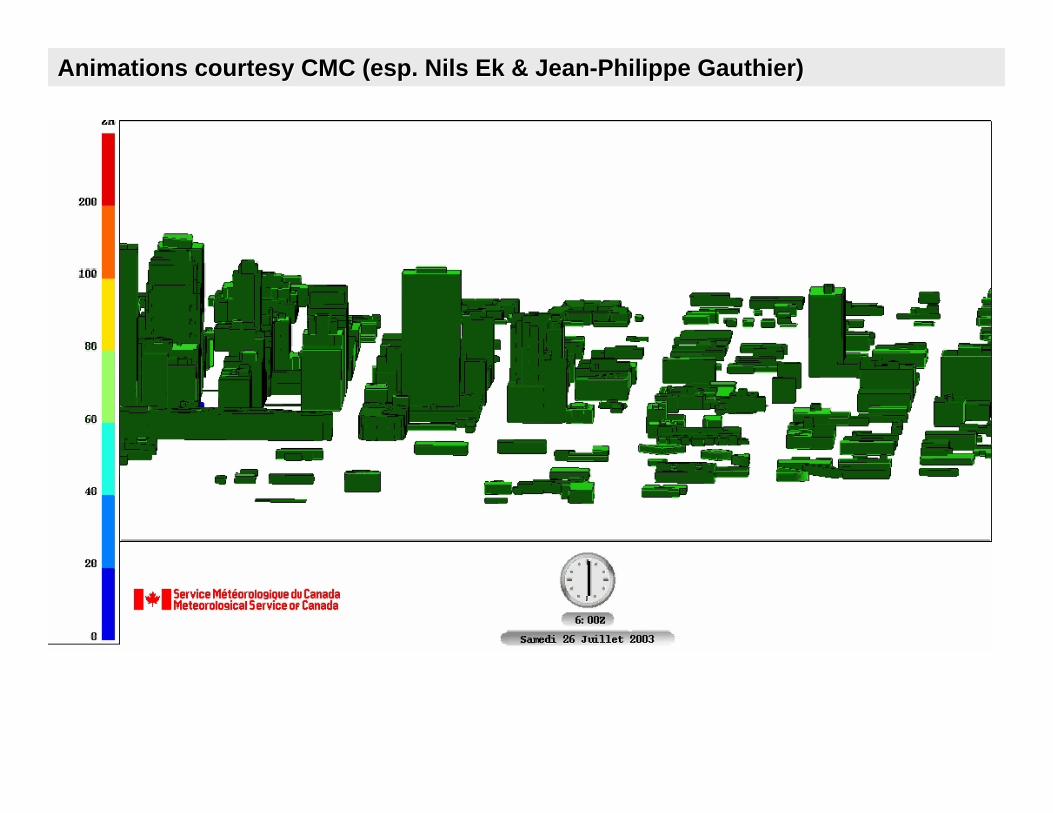
Animations courtesy CMC (esp. Nils Ek & JeanAnimations courtesy CMC (esp. Nils Ek & Jean--Philippe Gauthier)Philippe Gauthier)

800 900 1000 1100y [m]

2000

2100

2200

2300

2400

2500

2600

2000

8000

1400

0

600 700 800 900 1000 1100 1200y [m] (Crosswind)

2000

2100

2200

2300

2400

2500

2600

2700

2800

2900

3000

3100

x [m

]

52 53 54 55 56

62 63 64 65 66

72 73 74 76

83 84 86

94 96

512 513514 515 516

517

N

22002400

26002800

x [m]

600800

10001200y [m]

0

5000

10000

15000

C [ppt]

0

5000

10000

15000

C [ppt]Sampler positions

source

Mean groundMean ground--level concentration [parts per trillion] from forward LS level concentration [parts per trillion] from forward LS simulationsimulation

1001 1002 1003 1004

expt (ppt)

1001

1002

1003

1004

urba

nLS

53

54

55

56

63

64

65

66

83

84

86

94

96

513

515

517

x 2

x ½

Comparing LS model with observed concentrationComparing LS model with observed concentration

Fraction of predictions within factor of two:• forwards 9/16• backwards 8/16• ignoring flow disturbance 2/16ignoring flow disturbance 2/16

mustmust account for account for flow disturbanceflow disturbance

ConclusionConclusion

• CRTI urban dispersion project hinges on wind modelling from the global down to street scale

• prototype modelling system runs at CMC - more realistic than, say, re-tuning Gaussian puff/plume model

• time permitting, we’ll later look at another application of Thomson’s 3D LS model, used to infer strength Q of a gas source enclosed by a windbreak (i.e. emitting into a very disturbed surface layer) from the measured downwind concentration