1

1

16.513 Control Systems

Tingshu Hu Office: Ball Hall 405 Phone: 4374 , Fax: 3027Email: tingshu@gmail.com Office Hours: 3:30-6pm, Thursdayhttp://faculty.uml.edu/thu/http://faculty.uml.edu/thu/controlsys/controlsys.html

2

Today:

Introduction− Motivation

− Course Overview

− Course project

− My research projects

Matrix Operations -- Fundamental to Linear Algebra

− Determinant

− Matrix Multiplication

− Eigenvalue

− Rank

2

3

1.1 Motivation What is a "system"?

– A physical process or a mathematical model of a physical process that relates one set of signals to another set of signals

Two general categories of signals/systems:– Continuous-time (CT) signals/systems

1. INTRODUCTION

t

y(t)

• Examples: Speed/car, current/circuit, temperature/room

• Described by differential eqs., e.g., dy/dt = ay(t) + bu(t)

• Signals themselves could be discontinuous. But defined

for each time instant.

System

input/excitation/cause

output/response/result

– Examples: Air conditioner, cars, DC-DC converters

4

– Discrete-time (DT) signals/systems

k

y(k)

• Examples: Money in a bank account, quarterly profit

• Sequence of numbers

• Input/output related by difference equations, e.g.,

y[k+1] = ay[k] + bu[k], (on a daily or monthly base)

– DT and CT are quite similar, and will be treated in parallel

The goal of “System Theory”:– Establish input/output relationship through models,– Predict output from input, know how to produce desired output– Alter input automatically (via controller) to produce

desired output

Controller Systeminput outputrequirement

3

5

Use physical laws to model/describe the behavior of the system:

– What are the components? What properties do they have?

dtdv

Ci,dt

diLv,Riv C

CL

LRR

– Relationship among the variables by physical law: • KCL: Current to a node = 0, iR= iC= iL= i.• KVL: Voltage across a loop = 0.

Example: A simple electric circuit~ Output

R L C u(t)

i(t)

~ Input

~

6

)()(1

: 00tuvdi

Cdt

diLRiKVL

t

– An integral-differential or differential equation

– Input-output description or external description

How to analyze the input-output relationship?– For example, find the output i(t) given u(t) and IC.

We can use Laplace transform Note: only effective for LTI systems

dt

tduti

Cdt

tdiR

dt

tidL

)()(

1)()(2

2

~ Output

R L C u(t)

i(t)

~ Input

~

4

7

Laplace Transform, A Quick Review

Converting linear constant coefficient differential equations into algebraic equations

Other properties– Differentiation in the frequency domain: tf (t) ()F '(s)

– Convolution: h(t)f (t) H(s)F(s)

– Time and frequency shifting: f (t-t0) u(t-t0) e-st0 F(s);

es0t f (t) F(s - s0)

0

)()()( dtetfsFtf st

)()()()( 22112211 sFasFatfatfa

ssFdtffssFtf /)()(),0()()(

Key Properties – Linearity:

– Derivative theorem:

8

– Time and frequency scaling: f (at) 1/a F(s/a) for a > 0

– Initial Value Theorem: f (0+) = lims sF(s)

– Final Value Theorem: f () = lims0 sF(s) if all the poles of sF(s) have strictly negative real parts

)()(1

: 0

0

tuvdiCdt

diLRiKVL

t

)(ˆ)(ˆ

)(ˆ)(ˆ 00 su

s

v

Cs

siisisLsiR

~ Output

R L C u(t)

i(t)

~ Input

~

Example (Continued)

5

9

1)(ˆ

1)(ˆ

200

2

RCsLCs

cvLCsisu

RCsLCs

cssi

Is there any pattern with the equation?– It has two components, one caused by input, and the

other by IC

How about the voltage across the capacitor?

An algebraic equation vs integral-differential equation. Solution:

1

)(ˆ1

1)(ˆ)(ˆ

200

20

RCsLCs

vRCLCsLisu

RCsLCss

v

Cs

sisv

s

vLisusi

csRLs 0

0)(ˆ)(ˆ1

What is the system's transfer function?

10

g(s) ^ ^ i(s) = g(s) u(s) u(s) ^ ^

^

– Frequency domain analysis

How to obtain the response in time domain?

Assume that the ICs are zero, then

)(ˆ)( 1 siLti

)s(u1RCsLCs

Cs)s(i

2

1RCsLCs

Cs)s(g

2

– Suppose that L = C = 1, R = 2, v0 = i0 = 0, and u(t) = U(t) (unit step function). Then

6

11

222 1s

1

1s2s

1

1RCsLCs

)s(uCs)s(i

s1

)s(u

tte)t(i

00.05

0.10.15

0.20.25

0.30.35

0.4

0 5 10 15

t

i(t) Does this make sense

for the circuit?

R L C u(t) v(t)

+

-

12

Limitation of Laplace transform: not effective for time varying/nonlinear systems such as

The state space description to be studied in this course will be able to handle more general systems� How can we do it?� Properties can be characterized without solving for

the exact output

)(),()(),()(),()( 01 tutybtytyatytyaty

To get some general idea about state space description,we consider the same circuit system.

7

13

~ Output

R L C u(t)

i(t)

~ Input

~

State-Space Description– State variables: Voltage across C and current through L

uLvLiLRdt

di

iCdt

dv

)/1()/1()/(

)/1(

v(t)

– state equation:

– A set of first-order differential equations

uLi

v

LRL

C

i

v

/1

0

//1

/10

14

It describes the behaviors inside the system by using the state variables v(t) and i(t)

How to describe the output?

i

viy 10

– The output equation

Combined with the state equation, we have the state-space description or internal description

~ Output

R L C u(t)

i(t)

~ Input

~ v(t)

i

vy

uLi

v

LRL

C

i

v

10

,/1

0

//1

/10

Cxy

BuAxx

x

A B

C

x

8

15

A general form:

qpn y

y

y

y

u

u

u

u

x

x

x

xtuxhy

tuxfx

2

1

2

1

2

1

,,,),,(

),,(

Main features of the state-space approach It describes the behaviors inside the system

Characterizes stability and performances without solving

the differential equations

Applicable to more general systems, nonlinear,

time-varying, uncertain, hybrid

Most recent advancements in control theory are developed via state-space approaches

16

Textbook:– Chi-Tsong Chen, Linear System Theory and Design,

3rd Edition, Oxford University Press, 1999 (Required)

Goals: To achieve a thorough understanding about systems theory and multivariable system design

1.2 Course Overview

9

17

Tentative Outline (12 lectures):

– Introduction

– The fundamentals of linear algebra

– Modeling: Use diff. equ. to describe a physical system

– Analysis:

• Quantitative: How to derive response for a given input

• Qualitative: How to analyze controllability, observability, stability and robustness without knowing the exact solution?

18

– Design:

• How to realize a system given its mathematical description

• How to design a control law so that desired output response is produced

• How to design an observer to estimate the state of the system

• How to design optimal control laws

– Continuous-time and discrete-time systems will be treated in parallel

10

19

Prerequisites:

– 16:413 Linear Feedback Systems

– Background on

• Linear algebra: Matrices, vectors, determinant,

eigenvalue, solving a system of equations

• Ordinary differential equations

• Laplace transform, and

• Modeling of electrical and mechanical systems

20

• Grading:

Homework 10%

Mid Term 35% (All by hand, computer/ calculator not allowed)

Project 25%

Final Examination 30%

All exams are open book, open notes

11

21

• General Rules:– Homework solutions will be provided together with lecture

notes, before submitted. – Make sure you understand everything you write down.– Homework due next class. – Project should be done independently.

• Attendance: will be taken occasionally. Positive attitude is a key to success.

• If you decide to do something, use your heart and do it well. Otherwise it will be a waste of time.

22

Course Project

Mu

y

A cart with an inverted pendulum (page 22, Chen’s book)

u: control input, external force (Newton)y: displacement of the cart (meter) angle of the pendulum (radiant)

The control problems are1: Stabilization: bring the pendulum to the inverted position and keep it there.

Assume the angle is initially small enough. 2: Assume the pendulum is initially downward. Design a control algorithm to

bring it upward and keep inverted.Assume that there is no friction or damping. The nonlinear model is as follows.

θg

θθmlu

θ

y

lθ

θmlmM

sin

sin

cos

cos 2

m

: mass of the pendulum

: length of the pendulum

: mass of the cart, g 9.8

m

l

M

12

23

1. Derive a linear model for the system.2. Design feedback laws using Matlab.3. Validate your designs with Simulink and animation.

Problems:

Next, I will describe some control systems in the lab (BL406).

24

A one –dimensional magnetic suspension test rig

This experiment is part of the NSF project: (Sept. 06 – Aug. 10). The control objective is to keep the free end of the beam suspended. The gap between the beam and the electromagnet follows any set value via a nonlinear controller, which is implemented by a microprocessor,or the Labview. An eddie-current sensor converts the gap into a voltage signal which is fed into the microprocessor; The controller in the microprocessor computes the desired currents and output it to a power amplifier.

13

25

The beam rests on the stator when the controller is turned off

The beam suspended when a nonlinear feedback control is applied.

26

The robust controller adjusts the current of the electromagnet so that the gap is maintained at the same set value under different load

14

27

A two dimensional suspension system

28

A power electronic converter: buck-boost DC-DC converter

Supported by NSF Sept. 2009 – Aug. 2012

15

29

Pulse-widthmodulator

D

Q1D1

L

C R

+

v

vg

RL

i

When MOSFET is on When MOSFET is off

C R

+

v

vg

RL

i

onR

L

C R

+

v

vg

RL

i

Dv

D

g

Lon

v

vLv

i

RC

L

RR

dt

dvdt

di

00

01

10

01

10

1 10 0

L

g

D

di Rvidt L L

Lvdv v

C RCdt

D= 0.2

D= 0.5

D= 0.8

State space description

30

Simulink with switching model

16

31

Simulink with averaged model

T. Hu, "A nonlinear system approach to analysis and design of power electronic converters with saturation and bilinear terms," IEEE Trans. Power Electronics, 26(2), pp.399-410, 2011.

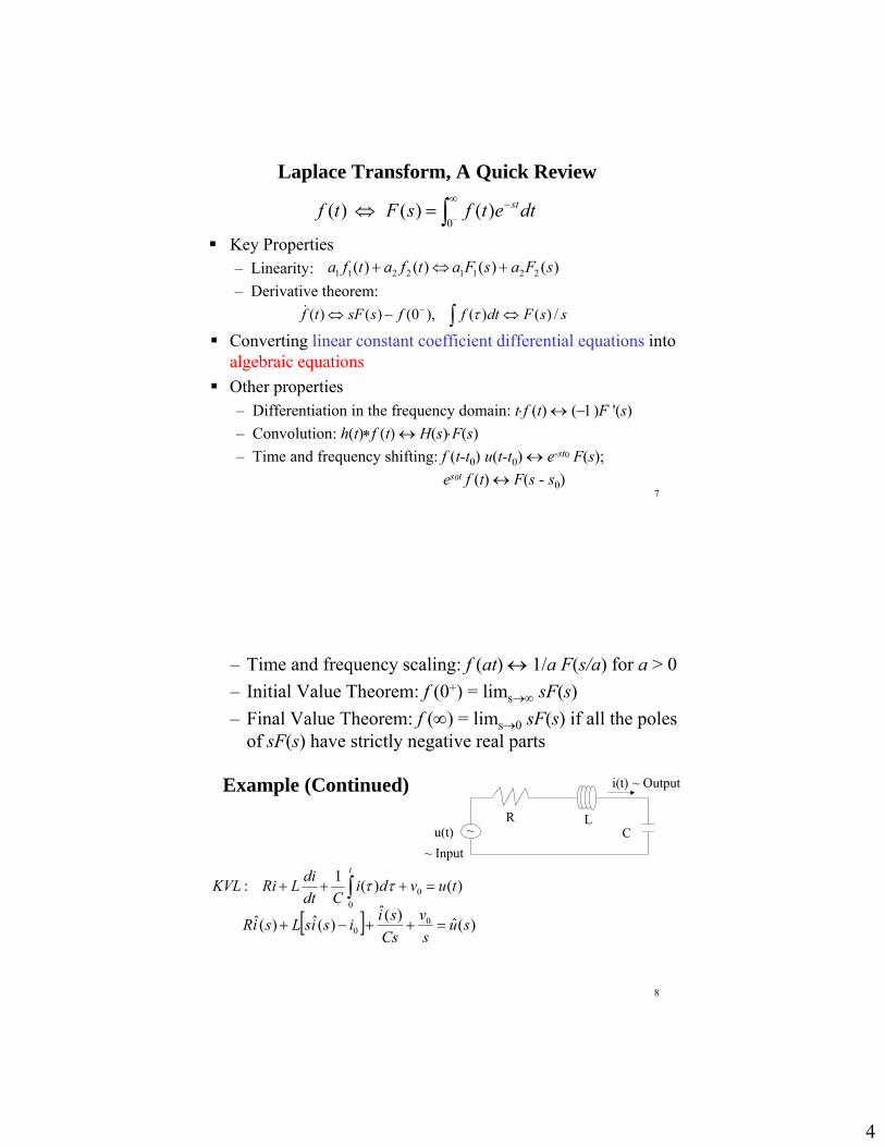
Power systems driven by battery/supercapacitor hybrid energy storage devices (Funded by NSF)

17

33

Load driven by battery/supercapacitor hybrid

u1

u2

ov

ibat

isc

Control inputs: u1,u2 (duty cycle)Output: ibat, isc, vo

Control objective: Given reference ibat,ref, vo,ref, design controllaw for u1,u2 so that ibat follows ibat,ref, vo follows vo,ref.

Bidirectional buck-boostDC-DC converter

34

State space description: Let x be state variable, x =[v1,v2,vsc,iL1,iL2,vo]’. Then

0 1 1 2 2x A x A xu A xu

A0=[-1/Re/C1 0 0 -1/C1 0 00 -1/Ru/C2 1/Ru/C2 0 -1/C2 00 1/Ru/Cu -1/Ru/Cu 0 0 0

1/L1 0 0 -(RL1+Ron)/L1 0 -1/L1

0 1/L2 0 0 -(RL2+Ron)/L2 -1/L2

0 0 0 1/Co 1/Co -1/R/Co]

A1=[0 0 0 0 0 00 0 0 0 0 00 0 0 0 0 00 0 0 0 0 1/L1

0 0 0 0 0 00 0 0 -1/Co 0 0]

A2=[0 0 0 0 0 00 0 0 0 0 00 0 0 0 0 00 0 0 0 0 00 0 0 0 0 1/L2

0 0 0 0 -1/Co 0]

18

35

36

0 0.02 0.04 0.06 0.08 0.1 0.12 0.14 0.16 0.18 0.20

1

2

3

4

5

6

7

8

9

Tracking ibat,ref =1.5A, v0,ref = 7V

19

37

A boost converter controlled by a microcontrollerThe controller is constructed using Matlab/Simulink, Then written into the microprocessor Funded by NSF.

Circuit Theory I, Copyright of Tingshu Hu 38

My summer project: A high efficient high performance LED driver with dimming control

20

39

Today:

Introduction− Motivation

− Course Overview

− Course project

− Control systems in my research projects

Matrix Operations -- Fundamental to Linear Algebra

− Determinant

− Matrix Multiplication

− Eigenvalue

− Rank

40

Operations on Matrices The classical control theory is based on Laplace

transform and z-transform also called frequency-domain approach

The modern control theory is established uponLinear Algebra State-space approach, or time domain approach

A linear time invariant system can be described as

)t(Du)t(Cx)t(y

)t(Bu)t(Ax)t(x

Systems properties all characterized with the matricesA,B,C,D.

21

41

2 by 2 (or 2×2) matrices: 11 12

21 22

1 2 ,1 3a aa a

A 2 by 3 matrices: ,a b cd e f

A 3 by 2 matrix: a bc de f

An n×m matrix: 11 12 1

21 22 2

1 2

m

m

n n nm

a a aa a a

a a a

Matrices: Square or non-square

Addition and subtraction: element by element

Multiplication is not by element.

n: the number of rows; m: the number of columns.

n×1: a column vector; 1×m : a row vector.

aij: element at the i-th row,j-th column

42

Matrix Multiplication:

Product of a 1×n matrix a n×1 matrix is a scalar. Product of a n×1 matrix and a 1×n matrix is an n×n matrix

a b x ax bycx dyc d y

a b u x au bv ax bycu dv cx dyc d v y

x

a b c y ax by czz

x xa xb xcy a b c ya yb ycz za zb zc

Generally, A B B A

• You cannot multiply any two matrices. They have to be compatible:to get AB, the number of columns of A must equal to the numberof rows of B, e.g., A: k×n, B: n×m.

22

43

Let A be a 3×4 matrix, B be a 4×2 matrix

1

2

3

1 2

1 2 3 45 6 7 8 ,9 10 11 12

[ ]

a eA b fA A B c gA d h

B B B

1 2 1 2

1 1 21 1

2 2 2 1 2

3 3 3 1 2

1 1 1 2

2 1 2 2

3 1 3 2

2 3 4 2 3 45 6 7 8 5 6 7 8

9 10 11 12 9 10 11 12

AB A B B AB AB

A B BA A BAB A B A B A B B

A A B A B B

A B A B a b c d e f g hA B A B a b c d e f g hA B A B a b c d e f g h

44

BA is defined only if the number of columns of B is theSame as the number of rows of A. Suppose

How about BA?

1

2

3

1 2

1 2 3 45 6 7 8 ,9 10 11 12

[ ]

a eA b fA A B c gA d h

B B B

1

1 2 3 2

3

1

1 2 3 2 1 1 2 2 3 3

3

, , thenA

B B B B A AA

ABA B B B A B A B A B A

A

But each B1A1, B2A2, B3A3 is a matrix.

Not defined at all for this case.

23

45

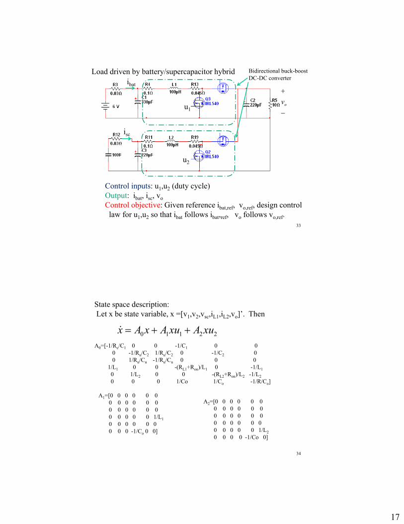
How about

1 11 2 1 2

2 2

? ?B AB

A A A B A B A BB AB

If A and B are compatible, (AB defined), then AB1 and AB2 arenot defined.

Be careful. Correct partition is important. Compatibility is essential.

Example: ?

11

10

01

20

11

46

Product of block partitioned matrices: Suppose that A and Bare partitioned compatibly as

,,2221

1211

2221

1211

BB

BBB

AA

AAA

Then

2222122121221121

2212121121121111

BABABABA

BABABABAAB

Compatibly partitioned means that the partition of the columns of A is the same as the partition of the rows of B

24

47

Determinant: A scalar defined for a square matrix

det ;

det

a b ad bcc d

a b cgec ahf dbaei dhc gd ibfe f

g h i

a b ca b c d e fd e f g h ig h i a b c

d e f

Exercise: 1 2 3

det 3 2 14 5 6

48

• Determinant of a triangular matrix:

det is the product of the diagonal elements.

All zero below the diagonal, or all zero above the diagonal

The determinant can be simplified by making the matrix a diagonalone through elementary operations that preserve the determinant.

If an entire row or an entire column is 0, the determinant is 0.

?

10000

9800

7650

4321

det

0 0 0

0 0det ?

0

a

e b

f h c

g i j d

Upper triangular Lower triangular

25

49

• Elementary operations that preserve the determinant:

1) Add one row scaled by a number to another row

Add row 1 to row 2

2) Add one column scaled by a number to another column

1 2 33 2 14 5 6

A

1 2 34 4 44 5 6

1 2 34 4 44 5 6

1 2 14 4 04 5 1

Add column 2 ×(-1) to column 3

1 2 14 4 04 5 1

1 2 14 4 03 3 0

Add row 1 × (-1) to row 3

1 2 14 4 03 3 0

Row 3 minus row 2×(3/4)1 2 14 4 00 0 0

03652484512

654

123

321

det)det(

A

(keep row 1)

(keep column 2)

(keep row 1)

50

• Determinant of the product of matrices:

det( ) det det

det( ) det det det

AB A B

ABC A B C

How about det(A+B), det(A-B)?

• Determinant of a block triangular matrix:

1

2

3

4

* * *0 * *det ?0 0 *0 0 0

AA

AA

Assume that A1,A2,A3,A4 are all square.

Examples: 1 2 9 102 2 1 3 4 11 12det 0 3 5 , det 0 0 5 60 4 6 0 0 7 8

26

51

1 2 3det 1 3 5

1 4 8

1 2 3det 0 1 2

1 4 8

1 2 3det 0 1 2

0 2 5

1 2 3det 0 1 2 1

0 0 1

r2-r1 r2

r3-r1 r3

r3-2r2 r3

An example:The column that is changedshould not be scaled by any number except 1;The row that is changed should not be scaled by any number except 1

52

Why elementary operations preserve the determinant?• Because elementary operation is equivalent to multiplying the

matrix with another one whose determinant is 1.

1 0 0Since det 0 1 0 1,

0 1

1 0 0det = det 0 1 0 det

0 1

x

a b c a b c a cx b cd e f d e f d fx e fg h i g h i g ix h ix

What about 1 0 00 1 0 ?

0 1

a b cd e fg h ix

ihg

fed

cbaAdd column 3 scaled by x to column 1

ihixg

fefxd

cbcxa

10

010

001

xihg

fed

cba

27

53

A square matrix is said to be nonsingular if its determinant is nonzero.

• If two rows (columns) are switched, the determinant changes the sign;

• If a whole row (column) is scaled by a number k, the determinantis scaled by a number k.

• What if the whole matrix is scaled by a number k?

0

det 0 1

1 1 0

det 1 1 1

3 4 1

x x

x

ax bx x c

Exercise:

54

Eigenvalue of a square matrix: s is an eigenvalue of A if

det[ ] 0sI A 1 0 00 1 0

0 0 1

I

If A is n×n, det[sI-A] is a polynomial of order n. An eigenvalueis a root of the polynomial. A has n eigenvalues.

2

0 1 ,2 3

1det[ ] det 3 2 ( 1)( 2)2 3

A

ssI A s s s ss

Roots are s1= 1 and s2 = 2.

Exercise: 1 22 1

0 1 00 0 11 3 3

28

55

The inverse of a square matrix: If det A0, A has a unique inverse X such that AX=XA=I, denoted as X=A

1 1,a b d bA Ac d c aad bc

Solving a system of equations:

1 1

1

a b x eax by ecx dy f c d y f

a b a b x a b ec d c d y c d f

x a b ey c d f

Exercise: What is the inverse of

cos sin ?sin cos

bAXbAX 1

56

The inverse of a block partitioned matrix:

2

1

0 A

BAA

12

111

0 A

XAA

for certain X. What is X ?

Assume that A1 and A2 are square and nonsingular, then

29

57

Sub-matrix of a matrix

1 2 3 45 6 7 89 10 11 12

1 3 49 11 12

a 2 by 3 matrix

1 2 3 45 6 7 89 10 11 12

1 3 45 7 89 11 12

a 3 by 3 square matrix

There are ? 3 by 3 sub-matrices? 2 by 2 sub-matrices12 1 by 1 matrices

58

Rank: The rank of M is the highest dimension of a square sub-matrix whose determinant is nonzero.denoted as (M), or, rank(M).

1 4 7 102 5 8 113 6 9 12

M

For example, a 34 matrix

33 sub-matrices22 submatrices11 sub-matrices

Suppose that • the number of 33 sub-matrices with nonzero det is N(3)• the number of 22 sub-matrices with nonzero det is N(2)• the number of 33 sub-matrices with nonzero det is N(1)

If N(3)0, then (M)=3If N(3)=0 and N(2)0, (M)=2If N(3)=N(2)=0 and N(1)0, (M)=1(M)=0 only if M=0

You need to work from the highest order submatrices.The procedure stops wheneveryou find one nonzero det.

? ? 12

30

59

400003200001

AExample 1:

33 submatrices:

8det 12det 0det 0det

;400020001

;400030001

;400032000

;000320001

4321

AAAA (A)=3

All the 33 submatrices have 0 det. And there is at leastone 22 nonsingular submatrix (A)=2

1

1 0 1 00 1 0 11 1 1 1

A

Example 2:

It can be very tedious to check all sub-matrices. A systematic way to find the rank is to use elementary operation

to transform the matrix into a special form,.e.g., block diagonal.

60

Elementary operations that preserve the rank:

400003200001

A

1) Add one row scaled by a number to another row

1 0 0 00 2 3 00 0 0 4

r1× 4+r3→r31 0 0 00 2 3 04 0 0 4

Add row 1 scaled by 4 to row 3

2) Add one column scaled by a number to another column

1 0 0 00 2 3 04 0 0 4

1 0 0 00 2 3 00 0 0 4

3) Exchange two columns or two rows

All operations that keep the determinantor scale the determinant by a nonzero number

(-1)c4+c1→c1

31

61

1 4 7 102 5 8 113 6 9 12

M

Add row 2 scaled by -1 to row 3: r2*(-1)+r3 → r3

1 4 7 102 5 8 111 1 1 1

Add row 1 scaled by -1 to row 2: r1*(-1)+r2→ r2

1 4 7 101 1 1 11 1 1 1

Add row 2 scaled by -1 to row 3

1 4 7 101 1 1 10 0 0 0

Rank < 3, but 1 4det 1 4 3 01 1

Rank = 2

62

• Suppose M is n×m. rank(M) min{m,n}• If M is multiplied with a nonsingular matrix (square and

has non-zero determinant), the rank is preserved. This is why elementary operations preserve the rank.

Since there are usually many sub-matrices, a systematic procedureto compute the rank is to use elementary operation to make it into upper or lower triangular form. Another simple operation that preserves the rank is to reorder the columns or rows (permutation).

31

2 1 1 2 3 2 3 1

3 2

;AA

A A A A A A A AA A

This operation is equivalent to multiplythe matrix with a matrixwhose determinant is 1 or -1.

1 1 11 2 31 3 51 4 7

Example:

?,

?,

2321

3321

YAYAAA

XAXAAA

32

63

Next Time :– Math. Descriptions of Systems

• Classification of systems• Linear systems• Linear-time-invariant systems• State variable description• Linearization

64You may use computer to check your answer.