Embed Size (px)
Citation preview

HAL Id: hal-00331836https://hal.archives-ouvertes.fr/hal-00331836
Submitted on 17 Oct 2008
HAL is a multi-disciplinary open accessarchive for the deposit and dissemination of sci-entific research documents, whether they are pub-lished or not. The documents may come fromteaching and research institutions in France orabroad, or from public or private research centers.
L’archive ouverte pluridisciplinaire HAL, estdestinée au dépôt et à la diffusion de documentsscientifiques de niveau recherche, publiés ou non,émanant des établissements d’enseignement et derecherche français ou étrangers, des laboratoirespublics ou privés.
Reusable containers within reverse logistic contextAfif Chandoul, Van-Dat Cung, Fabien Mangione
To cite this version:Afif Chandoul, Van-Dat Cung, Fabien Mangione. Reusable containers within reverse logistic context.2007. �hal-00331836�

1
Reusable containers within reverse logistic context
Chandoul Afifa,*, Van-Dat Cunga, Fabien Mangionea
a Laboratoire G-SCOP 46, avenue Félix Viallet - 38031 Grenoble Cedex 1 - France
Abstract
Due to economic and environmental constraints, many organizations have started to ship their products in reusable containers such as plastic pallets, boxes and crates. Minimizing the total flow cost arising from reusable containers is a major problem for these organizations. In this paper we will focus on the modeling of this problem as a network flow, and the proposal of an appropriate resolution method. This resolution method will allow us to better understand the system behavior and can be an important tool for studying related problems, such as dimensioning and purchasing policy.
Keywords: Reusable transport packages, network flow, optimization, container management, supply chain.
1. Introduction Since the mid-1980s, reusable containers have been adopted by many companies. In 1987, for example, the Bergen Brunswig Drug Company in California purchased 120,000 returnable plastic containers to replace one-use corrugated cartons. The company ships from its 37 distribution centers to its 10,000 pharmacies, located in 40 states (D.Saphire, 1994). Many other manufacturers in electronic goods and the automobile industry have also switched to reusable containers. This adoption is essentially due to potential economic benefits. It enables companies to save money by decreasing packaging material requirements: generally the cost of reusable containers is amortized over their lifecycle and the more the container is used the more the cost per trip is decreased. It reduces product damage due to shipping and handling because reusable containers are generally sturdier than one-way container and they are designed to withstand multiple uses thus providing better product protection. Other savings are possible. Warehouse utilization can be improved by reducing storage space requirements since reusable containers can be stacked higher than one-way containers. Improvements in worker safety can reduce costs since their ergonomic design reduces injuries from box cutters, staples, debris and stray packaging(D.Saphire, 1994). Furthermore, reusable containers are better for the environment since they reduce packaging waste. This can be a tool to meet the waste reduction requirements of government regulations, which are especially strict in EU countries (M.Kärkkäinen et al., 2004). However, reusing containers requires a more complex supply chain. The purchasing costs of reusable containers are significantly higher than those of one-way containers. A reusable container, such as a plastic box, can cost 10 times more than a one-way container, such as a corrugated box (D.Saphire, 1994). Therefore, for reusable containers to be of benefit, efficient container-management is a top priority. Despite the importance of specific container management, there are few academic studies on the subject. Those that do exist can be classified under 4 headings:
* Corresponding author. Tel. : +334 76 57 43 26 ; fax : +334 76 57 46 95. E-mail addresses: [email protected] (A.Chandoul), [email protected] (VD.Cung), [email protected] (F.Mangione)

2
- Organisational: these studies deal with the different issues related to the implementation of reusable container systems, like collaboration and cooperation between supply chain members. They, generally, stress the role of information systems(Chan et al., 2005; Chan, 2007; Eelco de Jong et al., 2004; M.Kärkkäinen et al., 2004) .
- Environmental: These studies present the environmental advantages of reusable containers compared to one-way containers(Gassel and F.J.M., 1998; González-Torre et al., 2004; S. Paul Singh et al., 2006b).
- Economic: in these studies, the economic benefits of reusable containers are shown compared to one-way containers. Often, these studies present the environmental advantages linked to economic benefits(Lerpong Jarupan et al., 2003; Martin, 1996; Orbis, 2004; Stopwaste and RPA, 2008).
- Operational: these studies propose mathematical tools that can help companies optimize the different aspects of their reusable container systems. We can find studies that propose models which optimize the total cost generated by the use of reusable containers (transport storage, maintenance…). Others deal with the problem of container depot localisation(ED Castillo and Cochran, 1996; Erera Alan L et al., 2005a; Erera Alan L et al., 2005b; I. A. Karimi et al., 2005; Leo Kroon and Gaby Vrijens, 1995).
In this paper we will deal with the operational side of the problem. We will consider a system that contains three kinds of site: customer sites, supplier sites and depots: A customer site is a facility that receives the loaded containers from a supplier site. After the containers have been emptied the customer can return them to depots or supplier sites for storage and reuse. A supplier site is a facility that receives empty containers from depots or customer sites in order to load and send them to customers. A depot is a place in which we store empty containers after they have been used by customers. Depots can supply suppliers with empty containers. We suppose that storage is also possible at customer and supplier sites. Our purpose in this work is to propose a model that optimizes the total cost resulting from transportation between sites and storage and to propose an original resolution method for some particular cases. This method is based on simple recurring formulas that can be easily solved for the different decisions variables. This can help us to better understand the system behaviour and, in turn, can help us deal with other related problems, such as system dimensioning and purchasing policies for reusable containers. The remainder of this paper is organized as follows. In section 2, we will present a literature review of the container management problem from the operational side. In this review we will concentrate on the work presented by Kroon and Vrijens (1995). In this work the authors present a step-by-step analysis of the operating policies of container management systems. This work will be a reference for our paper. In section 3, a description of our problem will be presented in detail and an optimization model, in the form of a network flow problem, will be developed. This model is a basic formulation of the case with several customer sites, several supplier sites and several depots under some simplifying assumptions. In section 4, we will simplify the model and treat the case of one customer site, one supplier site and one depot. In this section an original resolution method will be developed. In section 5, a result analysis and interpretation will be presented. In the final section, we will outline our future intentions for extension and enhancement of the presented model. 2. Literature Review Most of the existing works have focused on sea container management. This is due to their large cost. One of the problems which has been studied is container repositioning. Karimi et

3
al. (2005) presented a new linear programming methodology based on a continuous-time approach which they called the event-based “pull” approach. In this continuous-time representation, the principle is to fix all possible event times a priori, taking into account some simplifications and assumptions. Initially, a chronologically ordered superlist of possible instances is generated identifying which container movements (events) may occur and the types of movements that may occur at each such instance. This superlist of times and events is then used to develop a linear programming (LP) formulation whose solution will define the events that minimize the total logistic (flow) cost. Erera et al. (2005) proposed two different formulations, one deterministic(Erera Alan L et al., 2005a), one stochastic(Erera Alan L et al., 2005b), for the same problem. In the deterministic formulation, they integrated container booking and routing decisions with repositioning decisions in the same model. They believe that a container operator who uses this formulation via a global system may indeed be able to reduce costs and improve equipment utilization as compared to the standard approaches which ignore container routings. In the Stochastic formulation they presented a stochastic model in which uncertain parameters are assumed to fall within an interval around a nominal value and they established some conditions for robust flow under certain definitions. Similar work has been developed in the soft drinks field for the returnable bottle. Del Castillo and Cochran (1996) modelled the reusable bottle production and distribution activities of a Soft Drink Company. They optimized the problem in terms of increasing the number of empty bottles available in order to make the comany more competitive. This is an alternative to the total cost optimization when cost calculation is not possible. It is important to note that the majority of texts deal with the problem in specific cases (sea containers or returnable bottles). The only text that we found that considers the problem in the general case is the paper of Kroon and Vrijens (1995). In this paper, the authors classified returnable container systems into three groups depending on their operating policies: switch pool systems, systems with return logistics, and systems without return logistic. In a switch pool system, participants have their own allotments of containers. Thus the cleaning, maintenance and storage are the responsibility of each pool-participant. Pool-participants may be the senders and recipients, or the senders, carriers, and recipients of the goods. If only the sender and the recipients are allotted containers, a transfer will take place when the goods are delivered to the recipient. In this case, the role of the carrier is to transport the loaded container to the recipients and to return the empty containers to the sender. Alternatively, the carrier is also allotted containers and replaces the loaded containers with empty containers when it picks up a load from a sender or recipient. In a system with return logistics, the containers are owned by a central agency. It is responsible for returning the containers after they are unloaded. There are two variants of this system.
• Transfer system: the core of this system is that the sender always uses the same containers. He is responsible for tracking, tracing, maintaining, cleaning and storing them.
• Depot system: Under the depot system, the empty containers that are not in use are stored at container depots, which can supply the senders with empty containers on demand.
In the last system, the system without return logistics, the containers are owned by a central agency, and the sender rents them for fixed periods. The containers return to the agency after use. The sender is responsible for return logistics, cleaning, maintenance, storage and control. In the same paper, Kroon and Vrijens (1995) proposed a mathematical model for the design of a return logistics system for returnable containers with a depot system variant. The main purpose of the model is to determine the suitable number of containers, the appropriate number of container depots and their locations in order to minimize the total cost.
4
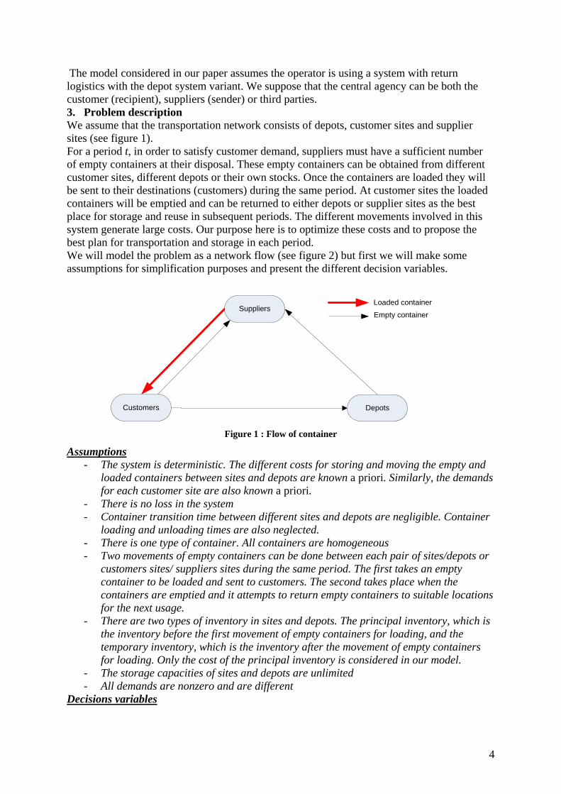
The model considered in our paper assumes the operator is using a system with return logistics with the depot system variant. We suppose that the central agency can be both the customer (recipient), suppliers (sender) or third parties. 3. Problem description We assume that the transportation network consists of depots, customer sites and supplier sites (see figure 1). For a period t, in order to satisfy customer demand, suppliers must have a sufficient number of empty containers at their disposal. These empty containers can be obtained from different customer sites, different depots or their own stocks. Once the containers are loaded they will be sent to their destinations (customers) during the same period. At customer sites the loaded containers will be emptied and can be returned to either depots or supplier sites as the best place for storage and reuse in subsequent periods. The different movements involved in this system generate large costs. Our purpose here is to optimize these costs and to propose the best plan for transportation and storage in each period. We will model the problem as a network flow (see figure 2) but first we will make some assumptions for simplification purposes and present the different decision variables.
Customers
SuppliersLoaded containerEmpty container
Depots
Figure 1 : Flow of container
Assumptions - The system is deterministic. The different costs for storing and moving the empty and
loaded containers between sites and depots are known a priori. Similarly, the demands for each customer site are also known a priori.
- There is no loss in the system - Container transition time between different sites and depots are negligible. Container
loading and unloading times are also neglected. - There is one type of container. All containers are homogeneous - Two movements of empty containers can be done between each pair of sites/depots or
customers sites/ suppliers sites during the same period. The first takes an empty container to be loaded and sent to customers. The second takes place when the containers are emptied and it attempts to return empty containers to suitable locations for the next usage.
- There are two types of inventory in sites and depots. The principal inventory, which is the inventory before the first movement of empty containers for loading, and the temporary inventory, which is the inventory after the movement of empty containers for loading. Only the cost of the principal inventory is considered in our model.
- The storage capacities of sites and depots are unlimited - All demands are nonzero and are different
Decisions variables

5
Let D be the number of depots (d=1, …, D), I be the number of customers sites (i=1,…, I), F be the number of Suppliers sites (f=1,…, F) and T be the number of periods in the planning horizon (t=1,…, T). We define the different decisions variables as follows:
• tfix : Number of loaded containers transported from suppliers f to a customer i at
period t • t
ix : Number of containers needed in customer site i at period t • t
ify : Number of empty containers transported from customer i to supplier f at period t to be loaded and sent to customers.
• tify 1 : Number of empty containers transported from customer i to supplier f at
period t to be returned to the suitable location. • t
dfz : Number of empty containers transported from depot d to suppliers f at period t to be loaded and sent to customers.
• tdfz 1 : Number of empty containers transported from depot d to suppliers f at
period t to be returned to the suitable location. • t
idu : Number of empty containers transported from customer i to depot d at period t to be loaded and sent to customers.
• tidu 1 : Number of empty containers transported from customer i to depot d at
period t for them to be returned to the suitable location. • t
ia : the principal inventory of containers in customer site i at period t. • t
ia 1 : the temporary inventory of containers in customer site i at period t. • t
dd : the principal inventory of containers in depot d at period t. • t
dd 1 : the temporary inventory of containers in depot d at period t. • t
fb : the principal inventory of containers in supplier site f at period t.
• tfb1 : the temporary inventory of containers in supplier site f at period t.
tfb
tdd t
dd1
tia t
ia1
tix
tfix
tfb1
tidu
tdfz
tify
1+tia
1+tfb
1+tdd
tify1
tdfz1
tidu1
Figure 2 : Network flow
Constraints
6
The constraints of the system are essentially the flow conservation constraints. They can be classified into four categories:
• the first represents the conservation flow before sending the loaded containers to different sites and depots
ti
d
tid
f
tif
ti auya 1++= ∑∑ ],0[,],0[ IiTt ∈∀∈∀ ( 1 )
∑∑∑ −−+=d
tdf
i
tif
tf
i
tfi
tf zybxb 1 ],0[,],0[ FfTt ∈∀∈∀ ( 2 )
∑∑ −+=i
tid
td
f
tdf
td udzd 1 ],0[,],0[ DdTt ∈∀∈∀ ( 3 )
For example, constraint ( 1 ) represents the conservation flow at customer site i at period t; the principal inventory t
ia is equal to the sum of departures from site i to depots ∑d
tidu and
supplier sites ∑f
tify plus the temporary inventory t
ia1 .
• The second category of constraints represents the conservation flow after the emptying of loaded containers and their return to different sites.
∑∑ −−+=+
d
tid
f
tif
ti
ti
ti uyaxa 1111 ],0[,],0[ IiTt ∈∀∈∀ ( 4 )
tf
d i
tif
tdf
tf byzb 111 111 ++=∑ ∑ −−+ ],0[,],0[ FfTt ∈∀∈∀ ( 5 )
∑∑ −+=+
f
tdf
td
i
tid
td zdud 1111 ],0[,],0[ DdTt ∈∀∈∀ ( 6 )
• The third category represents the sum of containers arriving at a customer site i at period t.
∑ =if
ti
tfi xx
,
],0[,],0[ IiTt ∈∀∈∀ ( 7 )
• The last category of constraint is the lower band constraint, that is the sum of arriving containers must be greater than or equal to the demand at site i.
ti
ti x≤δ ],0[,],0[ IiTt ∈∀∈∀ ( 8 )
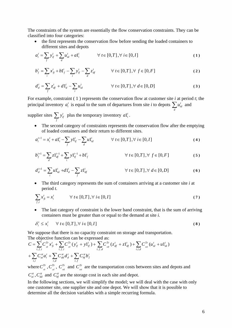
We suppose that there is no capacity constraint on storage and transportation. The objective function can be expressed as:
tf
ft
stbf
td
dt
stdd
ti
it
stai
dit
tid
tid
Tr
dft
tdf
tdf
Trtif
tif
ift
Trtfi
ift
Tr
bCdCaC
uuCzzCyyCxCCuidzdfyifxfi
∑∑∑
∑∑∑∑+++
++++++=
,,,
,,,,,,,,)1()1()1(
where Trxfi
C , Tryif
C , Trzdf
C and Truid
C are the transportation costs between sites and depots and staiC , st
ddC and stbfC are the storage cost in each site and depot.
In the following sections, we will simplify the model; we will deal with the case with only one customer site, one supplier site and one depot. We will show that it is possible to determine all the decision variables with a simple recurring formula.

7
4. Studied case In this case we add the following assumptions to the system (see figure 3):
• We have one customer site, one supplier site and one depot • We assume that the depot has the lowest cost, followed by the customer site and the
supplier site being the most expensive. The configuration of cost is as follow stb
sta
std CCC <<
• the initial stock of empty containers at the supplier site is equal to zero
Customers
SuppliersLoaded containerEmpty container
Depots
xt
tatt yy 1+
tt uu 1+
tt zz 1+
td
tb
Figure 3 : Decision variables
The different constraint can be simplified as follows
tttt auya 1++= ttttt zybxb −−+= 1
tttt udzd −−= 1 ttttt uyaxa 1111 −−+=+
tttt byzb 1111 ++=+ tttt zdud 1111 −+=+
ttx δ≥ The objective function is given by
t
t
stb
t
t
std
t
t
sta
t
tttr
t
tttrtt
t
trtfi
t
tr bCdCaCuuCzzCyyCxCCuzyx ∑∑∑∑∑∑∑ +++++++++= )1()1()1(
Now we model the problem graphically as a network R=(X, U, a, b, c) for use in the different proofs. X: Set of nodes that represents the three sites at each period t U: Set of arcs joining nodes. These arcs can be storage arcs or transportations arcs. Each arc represent a decision variable and takes the same notation but in the capital form. For example, the arc which correspond to ty take the notation of tY .
a (u) : represent the cost of an arc Uu∈ . For example, try
t CYa =)( b(u) : represent the lower band of arc Uu∈ . All arcs have a lower band equal to zero
except tX arcs which have tδ as lower bands.

8
],0[)()(
)/(0)(Tt
XuubXUuubtt
t
∈⎪⎩
⎪⎨⎧
=∀=
∈∀=
δ
c(u) : represents the capacity of an arc. We suppose that it is infinite on all arcs
∞=∈∀ )(ucUu The different pairs of variables and arcs are shown with the corresponding arrow on figure 4 below. In the remainder of this work, the majority of the properties will be demonstrated using the minimum cost network flow theorem. This theorem states that a necessary and sufficient condition for a feasible solution f to be optimal on a network R=(X, U, a, b, c) is that for each cycle −+ Γ∪Γ=Γ such that
{ } 0)]()([;)]()([ >−−= −+ Γ∈Γ∈ubufMinufucMinMin
uuγ
it is necessary that 0)()( ≥−∑∑ −+ Γ∈Γ∈ uuuaua
)1,1( 11 −− tt uU
)1,1( 11 −− tt zZ
)1,1( 11 −− tt yY
),( tt uU
),( tt zZ
),( tt yY
),( tt aA
),( tt bB
),( tt cC
)1,( tt bB
)1,1( 1 tcC
),( tt xX ),( 11 ++ tt xX
)1,1( tt aA
)1,( tt uU
)1,( tt zZ
)1,( tt yY
),( tt uU
),( tt zZ
),( tt yY
),( 11 ++ tt aA
),( 11 ++ tt bB
),1( 11 ++ tt cC
)1,1( 11 ++ tt bB
)1,1( 11 ++ tt cC
)1,1( 11 ++ tt aA
)1,1( 11 ++ tt uU
)1,1( 11 ++ tt zZ
)11( 11 ++ tt yY
Figure 4 : Network flow illustration
Before resolving this problem we will define some new integer parameters, which will help us later when demonstrating properties. The first parameter is the principal threshold, a
dN . This parameter will help us to decide whether or not to send surplus empty containers from the customer to the depot for storage and reuse in the following a
dN periods. The second parameter is the secondary threshold, a
dM . This parameter will show whether sending the container from the customer to the depot for storage without reuse is better then keeping it at the customer site in the following a
dM periods. Definition 1. in the case when we have TrTrTr
zuyCCC +< , we define the principal-storing-
threshold of the customer to the depot, the integer adN , such that:
⎪⎩
⎪⎨⎧
+×++>+×+
+×+<+×Trst
dad
TrTrsta
ad
Trstd
ad
TrTrsta
ad
zuy
zuy
CCNCCCN
CCNCCCN
)1()1(
Remark 1. Figure 5 represent an illustration of definition 1. The first term of the first inequality Trst
aad y
CCN +× represents the cost of path ),,...,1,( 11,
−+−++ =Γad
ad
ad
NtNtttNt
YAAA , in
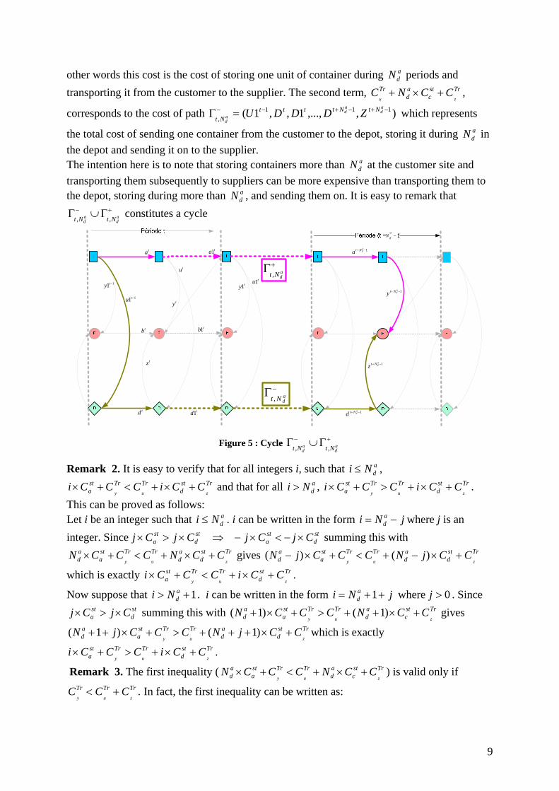
9
other words this cost is the cost of storing one unit of container during adN periods and
transporting it from the customer to the supplier. The second term, Trstc
ad
Trzu
CCNC +×+ ,
corresponds to the cost of path ),,...,1,,1( 111,
−+−+−− =Γad
ad
ad
NtNttttNt
ZDDDU which represents
the total cost of sending one container from the customer to the depot, storing it during adN in
the depot and sending it on to the supplier. The intention here is to note that storing containers more than a
dN at the customer site and transporting them subsequently to suppliers can be more expensive than transporting them to the depot, storing during more than a
dN , and sending them on. It is easy to remark that +− Γ∪Γ a
dad NtNt ,,
constitutes a cycle
11 −tu
tu
ty
tz
ta ta1
tb1tb
td td1
11 −tytu1ty1
1−a
dN
+Γ adNt ,
−Γ adNt ,
1−+ adNty
1−+ adNtz
1−+ adNta
1−+ adNtd
Figure 5 : Cycle +− Γ∪Γ a
dad NtNt ,,
Remark 2. It is easy to verify that for all integers i, such that adNi ≤ ,
Trstd
TrTrsta zuy
CCiCCCi +×+<+× and that for all adNi > , Trst
dTrTrst
a zuyCCiCCCi +×+>+× .
This can be proved as follows: Let i be an integer such that a
dNi ≤ . i can be written in the form jNi ad −= where j is an
integer. Since std
sta
std
sta CjCjCjCj ×−<×−⇒×>× summing this with
Trstd
ad
TrTrsta
ad zuy
CCNCCCN +×+<+× gives Trstd
ad
TrTrsta
ad zuy
CCjNCCCjN +×−+<+×− )()(
which is exactly Trstd
TrTrsta zuy
CCiCCCi +×+<+× .
Now suppose that 1+> adNi . i can be written in the form jNi a
d ++= 1 where 0>j . Since std
sta CjCj ×>× summing this with Trst
cad
TrTrsta
ad zuy
CCNCCCN +×++>+×+ )1()1( gives Trst
dad
TrTrsta
ad zuy
CCjNCCCjN +×+++>+×++ )1()1( which is exactly Trst
dTrTrst
a zuyCCiCCCi +×+>+× .
Remark 3. The first inequality ( Trstc
ad
TrTrsta
ad zuy
CCNCCCN +×+<+× ) is valid only if TrTrTrzuy
CCC +< . In fact, the first inequality can be written as:

10
TrTrTrstd
sta
ad yzu
CCCCCN −+<−× )( . Given that 0)( >−× std
sta
ad CCN consequently
TrTrTrzuy
CCC +< . Otherwise, TrTrTrzuy
CCC +> would give Trstd
Trsta
Trzuy
CCCCC ++>+ . In this case it is simple to see that if we have stock at the customer site at the end of period t it will be better to send all of it to the depot for storage and reuse. Definition 2. We define the secondary-storing-threshold of the customer to the depot, the integer a
dM , such that:
⎪⎩
⎪⎨⎧
×++>×+
×+<×std
ad
Trsta
ad
std
ad
Trsta
ad
CMCCM
CMCCM
u
u
)1()1(
Remark 4. This definition (see figure 6) shows that for a number of periods, i.e. greater than a
dM , storing stock at the customer site will be more expensive than sending it to the depot for storage without reuse. The two parameters a
dM and adN will help us to establish the
different properties.
11 −tu
tu
ty
tz
ta ta1
tb1tb
td td1
11 −tytu1ty1
1−a
dM
+Γ adMt ,
−Γ adMt ,
1−+ adMty
1−+ adMtz
1−+ adMta
1−+ adMtd
Figure 6 : +Γ a
dMt , and −Γ a
dMt ,
Property 1. For all ],0[ Tt∈ , 011 == tt zy
Proof. Suppose there exists a ],0[ Tt∈ such that 01 ≠tz , and hence 01 ≠+tb . Let −+ ΓΓ=Γ ttt U be a cycle composed of 4 arcs (see Figure 7) such that:
−Γt =( ),1 1+tt BZ
+Γt =( ), 11 ++ tt ZD
ty1
1+ta
1+tb
1+td
tz1
tu1
1+ty
1+tz
1+tu
Figure 7 : Cycle −+ ΓΓ tt U

11
We have )]()([ ubufMintu
−−Γ∈ because 01 >tz and 01 >+tb . In addition,
0)]()([ >−+Γ∈ufucMin
tu because the capacities of arcs are unlimited. Therefore,
{ } 0)]()([;)]()([ >−−= +− Γ∈Γ∈ufucMinubufMinMin
tt uuγ and according to the minimum
cost network flow theorem we must have that 0)()( ≥−∑∑ −+ Γ∈Γ∈ tt uuuaua . However, in this
case ∑ +Γ∈+=
tutrz
std CCua )( < st
btrzu
CCuat
+=∑ −Γ∈)( which is absurd, therefore tz1 must
equal zero, i.e. for all ],0[ Tt∈ ⇒ 01 =tz .
The same reasoning can be applied to ty1 .
Suppose there exists a ],0[ Tt∈ such that 01 ≠ty , and hence 01 ≠+tb . Let −+ ΓΓ=Γ ttt U be a cycle composed of 4 arcs (see Figure 8) such that:
−Γt =( ),1 1+tt BY
+Γt =( ), 11 ++ tt YA
ty1
1+ta
1+tb
1+td
11 −tz
tu1
1+ty
1+tz
1+tu
Figure 8 : Cycle −+ ΓΓ tt U
We have )]()([ ubufMintu
−−Γ∈ because 01 >ty et 01 >+tb . In addition,
0)]()([ >−+Γ∈ufucMin
tu because the capacities of arcs are unlimited. Therefore,
{ } 0)]()([;)]()([ >−−= +− Γ∈Γ∈ufucMinubufMinMin
tt uuγ and according to the minimum
cost network flow theorem we must have that 0)()( ≥−∑∑ −+ Γ∈Γ∈ tt uuuaua . However, in this
case try
stau
CCuat
+=∑ +Γ∈)( < st
btryu
CCuat
+=∑ −Γ∈)( which is absurd, therefore 01 =ty for all
],0[ Tt∈ . Remark 5. Property 1 implies that the stock at the supplier site will remain equal to zero if we begin with a stock equal to zero at t=0 . Property 2. For ],0[ Tt∈ ,if 01 ≠tu then ],1[ a
dNk∈∀ , 0=+ktz
Proof. Suppose there exists a ],0[ Tt∈ such that 01 ≠tu .
Let kt ,Γ be a cycle with ],0[ Tt∈ and ],1[ adNk∈ (see figure 9). Suppose that
−+ Γ∪Γ=Γ ktktkt ,,, , where ),,...,( 1,
ktkttkt YAA ++++ =Γ , is the path composed of the storage arcs
between t+1 and t+k and the transportation arc between the customer and the supplier. ),,..,,1( 1
,ktkttt
kt ZDDU +++− =Γ is the path composed of the transportation arc from the customer to the depot at period t, the storage arcs at depot between t+1 and t+k and the transportation arc from the depot to the supplier at period t+k .

12
+Γ kt ,
−Γ kt ,
tu1
1+tu
1+ty
1+tz
1+ta 11 +ta
11 +tb1+tb
1+td 11 +td
ktu +−11ktu +
kty +
ktz +
kta + kta +1
ktb +1ktb +
ktd + ktd +1
kty +−11
ktz +−11
ty1
tz1
Figure 9 : Cycle −+ Γ∪Γ ktkt ,,
Suppose there exists a 0≠+ktz which is the first non-zero occurrence, that is if 1>k then for all ]1,1[ −∈ ki we have 0=+itz . For, the case when k=1, 1+tz is the first and only non-zero occurrence. Therefore, all itd + and jtd +1 will be non-zero for ],1[ ki∈ for all k and
]1,1[ −∈ kj for k>1 because there are no units leaving the depot since, according to property 1, 01 =tz and 01 =ty for all t. Consequently, all arcs of path ),,...,,1( 1
,ktkttt
kt ZDDU +++− =Γ will have non-zero values, and thus 0)]()([
,>−−Γ∈
ubufMinktu
and since 0)]()([,
>−+Γ∈ufucMin
ktuit follows that:
{ } 0)]()([;)]()([,,
>−−= +− Γ∈Γ∈ufucMinubufMinMin
ktkt uuγ . We Know that that
∑+Γ∈
=ktu
ua,
)( Trsta y
CCk +× and Trstd
Trzu
ktu
CCkCua +×+=∑−Γ∈ ,
)( this implies that
∑ ∑+Γ∈
−Γ∈<−
ktu ktuuaua
,,
0)()( which is absurd because according to definition 1 for all adNk ≤ ,
Trsta y
CCk +× < Trstd
Trzu
CCkC +×+ . Therefore, 0≠+ktz for all ],1[ adNk ∈ .
Property 3. If the initial stock at the supplier site is equal to zero, then for all ],0[ Tt∈ 01 == tt bb
Proof. We have that 00 =b because we began with zero stock at the supplier site and that 011 == tt zy t∀ , therefore, there is no entry at the supplier site at t=0. Assume that there
exists a ],1[ Tt∈ such that 0≠tb which is the first non-zero occurrence, i.e. that for all ]1,0[ −∈ ti 0=ib . According to property 1, 011 11 == −− tt zy and therefore, 01 1 ≠−tb . Given
that 01 ≠−tδ and 01 =−tb , it follows that )0,0(),( 11 ≠−− tt zy
1st case : if 01 ≠−ty
Let −+ ΓΓ=Γ tytyty ,,, U (see figure 10) be a cycle such that:
),,1(
),1,(1
,
11,
tttty
tttty
YAA
BBY−+
−−−
=Γ
=Γ

13
11 −tu ty
tz
ta
tb
td
11 −ty
1−tu
1−ty
1−tz
1−ta 11 −ta
11 −tb1−tb
1−td 11 −td
Figure 10 : Cycle −+ ΓΓ tyty ,, U
The path ),1,( 11,
tttty BBY −−− =Γ does not contain an arc of zero value, given that 01 ≠−ty and
01 1 ≠−tb . Consequently, 0)]()([,
>−−ΓubufMin
tyand given that 0)]()([
,>−+Γ
ufucMinty
it
follows that { } 0)]()([;)]()([
,,>−−= +− Γ∈Γ∈
ufucMinubufMinMintyty uu
γ .
Since ∑∑ −+ Γ∈Γ∈+=<+=
tyty ustb
tryu
try
sta CCuaCCua
,,)()( (given that st
astb CC > ) ⇒
0)()(,,
<−∑∑ −+ Γ∈Γ∈ tyty uuuaua this is absurd, therefore tb can never non-zero. Consequently,
given that 011 11 == −− tt zy it also follows that 01 1 =−tb .
2nd case: if 01 ≠−tz :
Let −+ ΓΓ=Γ tztztz ,,, U (see figure 11) such that:
),,1(
),1,(1
,
11,
ttttz
ttttz
ZDD
BBZ−+
−−−
=Γ
=Γ
Given that 01 ≠−tz , 01 1 ≠−tb and 0≠tb , it follows that 0)]()([,
>−−ΓubufMin
tz on
),1,( 11,
ttttz BBZ −−− =Γ . In addition, since 0)]()([
,>−+Γ
ufucMintz
it follows that
{ } 0)]()([;)]()([,,
>−−= +− Γ∈Γ∈ufucMinubufMinMin
tztz uuγ . In this case
∑∑ −+ Γ∈Γ∈+=<+=
tytz ustb
trzu
trz
std CCuaCCua
,,)()( (given that st
dst
b CC > ) ⇒
0)()(,,
<−∑∑ −+ Γ∈Γ∈ tztz uuuaua which is also absurd, therefore tb can never be null. Therefore,
given that 011 11 == −− tt zy it follows that 01 1 ==− tt bb ( 111 111 −−− ++= tttt byzb ).
Finally, for all ],0[ Tt∈ , 01 == tt bb

14
tu1 ty
tz
ta
tb
td
ty1
tu1
1−tu
1−ty
1−tz
ta 11 −ta
11 −tbtb
td 11 −td
ty1
Figure 11 : Cycle −+ ΓΓ tztz ,, U
Property 4. For all ],0[ Tt∈ , 0=tu Proof. Assume there exists a ],0[ Tt∈ such that 0≠tu . Therefore, 0≠ta . Let
−+ ΓΓ=Γ tututu ,,, U be a cycle (see figure 12) such that:
),1(
),(1
,
,
tttu
tttu
DU
UA−+
−
=Γ
=Γ
tu1 1+ty
1+tz
1+ta
1+tb
1+td
ty1
11 −tu
tu
ty
tz
ta ta1
tb1tb
td td1
11 −ty
Figure 12 : Cycle −+ ΓΓ tutu ,, U
Since 0≠tu , it also follows that 0≠ta , and as a consequence that 0)]()([,
>−−ΓubufMin
tu.
In addition, since 0)]()([,
>−+ΓufucMin
tu it follows that
{ } 0)]()([;)]()([,,
>−−= +− Γ∈Γ∈ufucMinubufMinMin
tutu uuγ .
However, since ∑∑ −+ Γ∈Γ∈
+=<+=tutu u
tra
truu
std
tru CCuaCCua
,,)()( ⇒∑ ∑+ −Γ∈ Γ∈
<−tu tuu u
uaua, ,
0)()( this is in
contradiction with the minimum cost network flow theorem, and therefore for all ],0[ Tt∈ 0=tu .
Property 5. For all ],0[ Tt∈ , ttx δ=

15
Proof. Assume there exists a ],0[ Tt∈ such that ttx δ> . According to property 5 , for all ],0[ Tt∈ , 01 == tt bb . Given that 0≠tδ (see assumptions above) it follows that
)0,0(),( ≠tt zy
1st case: if 0≠ty
Let −+ ΓΓ=Γ tytyty ,,, U (see figure 13) be a cycle such that:
tu1 1+ty
1+tz
1+ta
1+tb
1+td
ty1tu1
tu
ty
tz
ta ta1
tb1tb
td td1
ty1tx
Figure 13 : Cycle −+ ΓΓ tyty ,, U
Given that ttx δ> it follows that 0)]()([
,>−−Γ
ubufMinty
and since 0)]()([,
>−+ΓufucMin
tyit
also follows that { } 0)]()([;)]()([
,,>−−= +− Γ∈Γ∈
ufucMinubufMinMintyty uu
γ
According to the minimum cost network flow theorem we must have that 0)()(
,,≥−∑∑ −+ Γ∈Γ∈ tyty uu
uaua but given that ∑∑ −+ Γ∈Γ∈+=<=
iyty utrx
tryu
CCuaua,,
)(0)( (the cost
of arc tA1 is null) there is a contradiction. Therefore, in this case ttx δ= . 2nd case: if 0≠tz and 0=ty (if 0≠ty we return to case 1)
Let ity + , ],1[ tTi −∈ , or jtu +1 , ],0[ tTj −∈ , and be the first non-zero variable. For example, if ity + is the first non-zero variable then all mty + and ntu +1 (with ]1,1[ −∈ im and ]1,0[ −∈ in ) are zero. 1stsub-case: if ity + the first non-zero variable: Let −+ ΓΓ=Γ tztztz ,,, U (see figure 14) such that:
),,...,1(
),,...,,,(
,
1,
ititttz
ititttttz
ZDD
YAAXZ+++
+++−
=Γ
=Γ
)1(
),(
,
,
tty
ttty
A
XY
=Γ
=Γ+
−

16
tz
td1
ity +
itz +
tx
itd +
ita +
Figure 14 : Cycle −+ ΓΓ tztz ,, U
Given that ity + is the first non-zero variable, it follows that between t+1 and t+i no containers depart from the customer site, i.e. all arcs of −Γ tz , are nonzero. In addition, ttx δ> which simply means that 0)]()([
,>−−Γ
ubufMintz
. Therefore,
{ } 0)]()([;)]()([,,
>−−= +− Γ∈Γ∈ufucMinubufMinMin
tztz uuγ and given that
∑∑ −+ Γ∈Γ∈+×++=<+×=
iztz utry
sta
trx
trzu
trz
std CCiCCuaCCiua
,,)()( (Because st
astd CC < )
this is in contradiction with minimum cost network flow theorem. Therefore ttx δ> is impossible ⇒ ttx δ= in this case. 2ndsub-case: if jtu +1 is the first non-zero variable with 0>j . In this case all mty + and ntu +1 , for
],1[ jm∈ et ]1,0[ −∈ jn , are zero. Let −+ ΓΓ=Γ tztztz ,,, U (See figure 15) such that :
)1,,...,1(
)1,1,...,,,(
,
1,
jtjtttz
jtjtttttz
DDD
UAAXZ+++
+++−
=Γ
=Γ
In the case where j=0 the tow paths are reduced to
)1(
)1,,(
,
,
ttz
ttttz
D
UXZ
=Γ
=Γ+
−

17
tz
td1
jty +
jtz +
tx
jtd +
jta +
jtu +1
jtd +1
Figure 15 : Cycle −+ ΓΓ tztz ,, U
Because it is supposed that ttx δ> then, given that no containers depart from the customer until t+j, there are no zero arcs on the path −Γ tz , and the tX arcs have a value greater than the
lower band ( ttx δ> ). Therefore, 0)]()([,
>−−ΓubufMin
tz and since 0)]()([
,>−+Γ
ufucMintz
it
follows that { } 0)]()([;)]()([
,,>−−= +− Γ∈Γ∈
ufucMinubufMinMintztz uu
γ
Since, according to minimum cost network flow theorem, 0)()(,,
≥−∑∑ −+ Γ∈Γ∈ tztz uuuaua is a
condition for optimality, and given that ∑∑ −+ Γ∈Γ∈
+×++=<×=iztz u ua
trx
trzu d CCjCCuaCjua
,,)()( , this is absurd. Therefore, in this
case ttx δ= . 3rd sub-case: if all ity + and jtu +1 , ],1[ tTi −∈ and ],0[ tTj −∈ , are equal to zero, then after t all transportation variables will be equal to zero except kk xandz , ],[ Ttk ∈ . Now, suppose that the feasible flow f found in this case is optimal. Let f’ be another feasible flow obtained by transforming f by subtracting ttx δλ −= from )1,,...,1,,,( TTtttt AAAAXZ=Γ and adding it to )1,,...,1,(' TTtt DDDD=Γ . This gives a gain of ))()(( dzxa CtTCCCtT ×−−++×−×λ which implies that f is not optimal. Therefore, ttx δ> is impossible ⇒ ttx δ= . Property 6. If for ],0[ Tt∈ , )(max1
],1[kt
Nktt
ad
a +∈
≥+ δδ then
)(max11],1[
ktNk
tttad
au +∈
−+≤ δδ
Proof. Assume there exists a ],0[ Tt∈ such that )(max11],1[
ktNk
tttad
au +∈
−+> δδ and let
],1[ adNi∈ be the index corresponding to the position of maximum demand, in other words
itktNk ad
++∈= δδ )(max
],1[. So, according to property 2, if 01 ≠tu then ],1[ a
dNk∈∀ ktz + =0. In
other words, in the interval ],1[ adNtt ++ the system uses only the stock available at the
customer site. However, this stock is strictly lower than it+δ because )(max11
],1[1 kt
Nktttt
ad
uaa +∈
+ <−+= δδ and consequently the demand at t+i cannot be satisfied,
which is absurd. Therefore, )(max11],1[
ktNk
tttad
au +∈
−+≤ δδ .

18
Property 7. Let ],0[ Tt∈ and i∈ ],1[ abN represent the position index of maximal demand: this
means that itktNk a
d
++∈
= δδ )(max],1[ with i>1. If )(max1
],1[kt
Nktt
ad
a +∈
>+ δδ then we have:
01 =+ jtu for all ]1,1[ −∈ ij , 0≠+kta for all ],1[ ik∈ and 01 ≠+lta for all ]1,1[ −∈ il Remark 6. If i=1 (i is at the position of maximum demand), then 01 ≠+ta Proof. Let ],0[ Tt∈ and i∈ ],1[ a
bN such that itktNk a
d
++∈
= δδ )(max],1[
and assume
that )(max1],1[
ktNk
ttad
a +∈
>+ δδ . )(max11],1[
ktNk
tttad
au +∈
−+≤ δδ which means that the
customer stock at period tttt uaa 111 −+=+ δ is greater than or equal to )(max],1[
ktNk a
d
+∈
δ , i.e.
)(max11],1[
1 ktNk
ttttad
uaa +∈
+ ≥−+= δδ . Assume that there is a non-zero departure jtu +1 for
]1,1[ −∈ ij which is the first non-zero occurrence, i.e. all departures mtu +1 for ]1,1[ −∈ jm are null. Let +− Γ∪Γ=Γ be a cycle (see figure 16) such that
)1,...,,1()1,...,1,(
1
11
jttt
jttt
DDUUAA
+++
+++−
=Γ
=Γ
jty +
jtz +
tx
tu1 jtu +1
1+ta
1+td
jta +
jtd +
jta +1
jtd +1
11 +ta
11 +td
Figure 16 : Cycle −+ ΓΓ U
Since all mtu +1 are null, there are no departures from the customer site, this means that stock lta + for ],1[ jl ∈ can never decrease and will remain greater than )(max
],1[kt
Nk ad
+∈
δ . In
addition, for all ],1[ jk∈ kty + can never exceed )(max],1[
ktNk a
d
+∈
δ ⇒ 01 >=− +++ ktktkt aya .
Therefore, the path )1,...,1,( 11 jttt UAA +++− =Γ cannot contain a null arc, i.e. 0)]()([ >−−Γ
ubufMin , and because 0)]()([ >−+ΓufucMin , it follows that:
{ } 0)]()([;)]()([ >−−= +− Γ∈Γ∈ufucMinubufMinMin
uuγ
Since, ∑∑ −+ Γ∈Γ∈+×=<×+=
utru
stau
std
tru CCjuaCjCua )()( (because st
astd CC < ) this is
absurd and therefore there is no departure jtu +1 for ]1,1[ −∈ ij , and the stock kta + for ],1[ ik∈ can never decrease, i.e. )(max
],1[nt
Nnkt
ad
a +∈
+ ≥ δ . In addition, given that ltltnt
Nnya
d
+++∈
≥> δδ )(max],1[
for ]1,1[ −∈ il , it follows that 01 >−= +++ ltltlt yaa .
Consequently, for jtu +1 , ]1,1[ −∈ ij , 0≠+kta for all ],1[ ik∈ and 01 ≠+kta for all ]1,1[ −∈ il . Property 8. For a )],max(,0[ a
dad MNTt −∈ , if )(max1
],1[kt
Nktt
ad
a +∈
>+ δδ , then

19
)(max11],1[
ktNk
tttad
au +∈
−+= δδ
Proof. Let )],max(,0[ ad
ad MNTt −∈ such that )(max1
],1[kt
Nktt
ad
a +∈
>+ δδ and let i∈ ],1[ abN
such that the maximum demand position be defined as itktNk a
d
++∈
= δδ )(max],1[
. Assume that
)(max11],1[
ktNk
tttad
au +∈
−+< δδ . In other words, for the customer stock at period t+1,
)(max],1[
1 ktNk
tad
a +∈
+ > δ and because there is no departure (according to property 8,
01 =+ jtu for all ]1,1[ −∈ ij ), the stock will stay the same or increase at the customer site in ],1[ itt ++ . Therefore, we will find that at period it + , )(max
],1[kt
Nkit
ad
a +∈
+ > δ and given
that itity ++ ≤ δ , it follows that 01 >−= +++ ititit yaa . Therefore, for all ],1[ ik∈ , kta + and kta +1 will be nonzero. 1st case: assume there exists a ],[ a
dNij∈ such that 01 ≠+ jtu which is the first non-zero occurrence of jtu +1 . In other words, for all ]1,[ −∈ jim , mtu +1 are null. Let +− Γ∪Γ=Γ be a cycle (see figure 17) such that:
)1,...,,1()1,...,1,(
1
11
jttt
jttt
DDUUAA
+++
+++−
=Γ
=Γ
jty +
jtz +
tx
tu1 jtu +1
1+ta
1+td
jta +
jtd +
jta +1
jtd +1
11 +ta
11 +td
Figure 17 : Cycle −+ ΓΓ U
Given that the stock at the customer site will stay the same until the period t+j (the first departure is jtu +1 , ],[ a
dNij∈ ), it follows that all mta + and mta +1 for ],[ jim∈ are nonzero. Thus, 0)]()([ >−−Γ
ubufMin and since 0)]()([ >−+ΓufucMin this implies that
{ } 0)]()([;)]()([ >−−= +− Γ∈Γ∈ufucMinubufMinMin
uuγ . Given that:
∑∑ −+ Γ∈Γ∈+×=<×+=
utru
stau
std
tru CCjuaCjCua )()( (because st
astd CC < ) this is absurd.
Therefore, in this case )(max11],1[
ktNk
tttad
au +∈
−+< δδ is impossible.
2nd Case: suppose that there is no period ],[ adNij∈ such that 01 ≠+ jtu .
1st sub-case: assume there exists a adNk > such that 01 ≠+ktu or 0≠+kty which is the first non-
zero occurrence.
20
1) If 01 ≠+ktu is the first non-zero occurrence, then all ltu +1 for ]1,1[ −+∈ kNl ad and all mty +
for ],1[ kNm ad +∈ are equal to zero. In this case, let +− Γ∪Γ=Γ be a cycle such that:
)1,...,,1()1,...,1,(
1
11
kttt
kttt
DDUUAA
+++
+++−
=Γ
=Γ
(the same form of cycle as figure 16) Given that for all ],1[ a
dNn∈ , 01 ≠+nta and that there are no departures between periods t+ a
dN and t+k, it follows that, for all ],1[ kNm ad +∈ , mta + and mta +1 are non-zero and the
path )1,...,1,( 11 kttt UAA +++− =Γ does not contain a null arc, i.e. 0)]()([ >−−ΓubufMin . Since,
0)]()([ >−+ΓufucMin , it follows that
{ } 0)]()([;)]()([ >−−= +− Γ∈Γ∈ufucMinubufMinMin
uuγ
Given that ∑∑ −+ Γ∈Γ∈+×=<×+=
utru
stau
std
tru CCkuaCkCua )()( this is absurd. Therefore, the
inequality )(max11],1[
ktNk
tttad
au +∈
−+< δδ is impossible⇒ )(max11],1[
ktNk
tttad
au +∈
−+≥ δδ .
2 ) If kty + is the first non-zero occurrence, then all the other mtu +1 and mty + values, for ]1,1[ −+∈ kNm a
d , are equal to zero. Let +− Γ∪Γ=Γ be a cycle such that (see figure 18):
),,...,,1(),...,1,(
1
11
ktkttt
kttt
ZDDUYAA
++++
+++−
=Γ
=Γ
Given that 01 ≠+nta for ],1[ adNn∈ and that there are no departures between periods t+ a
dN and t+k, it follows that stocks mta + , for ],1[ kNm a
d +∈ , and nta +1 , for all ]1,1[ −+∈ kNn ad ,
will be non-zero and consequently 0)]()([ >−−ΓubufMin . Since, 0)]()([ >−+Γ
ufucMin it
follows that { } 0)]()([;)]()([ >−−= +− Γ∈Γ∈ufucMinubufMinMin
uuγ . Since,
∑∑ −+ Γ∈Γ∈+×=<+×+=
utry
stau
trz
std
tru CCkuaCCkCua )()( for a
dNk > this is absurd and in
contradiction with minimum cost network flow theorem.
tx
tu1
1+ta
1+tc
kta +
ktc +
11 +ta
11 +tc
kty +
ktz +
Figure 18 : Cycle −+ ΓΓ U
2nd sub-case: Assume that all ktu +1 and kty + are equal to zero for a
dNk > . Let f be the flow found in this case and suppose that it is optimal with the assumption that
)(max11 ],1[kt
Nkttt
ad
au +∈
−+< δδ .

21
Let 01)(max1],1[
>−−+= +∈
tktNk
tt ua adδδα and let f’ be a new flow obtained from f by
subtracting α from the path ),...,1,( 11 Ttt AAA ++=Γ and adding it to the path ),...,1,,1(' 11 Tttt DDDU ++=Γ . The total cost resulting from f ’ has a variation of
))()(( sta
std
stu CtTCtTC −−−+×α which is negative given that
ad
ad
ad MtTMNtT >−⇒>− ),max( . According to definition 2, for all
std
Trsta
ad CjCCjMj
u×+>×> , and consequently:
0))()(()()( <−−−−×⇒×−+>×− std
stu
sta
std
Trsta CtTCCtTCtTCCtT
uα . Therefore, the cost of
f’ is less than f and consequently if )(max11],1[
ktNk
tttad
au +∈
−+< δδ the flow cannot
be optimal and, therefore, the inequality )(max11 ],1[kt
Nkttt
ad
au +∈
−+< δδ is
impossible⇒ )(max11],1[
ktNk
tttad
au +∈
−+≥ δδ .
According to property 7 )(max11],1[
ktNk
tttad
au +∈
−+≤ δδ , and, therefore,
)(max11],1[
ktNk
tttad
au +∈
−+= δδ .
Property 9. If, )(max1],1[
ktNk
ttad
a +∈
≤+ δδ for a )],max(,0[ ad
ad MNTt −∈ , then 01 =tu
Proof. Let )],max(,0[ ad
ad MNTt −∈ such that )(max1
],1[kt
Nktt
ad
a +∈
≤+ δδ and assume
that 01 ≠tu . According, to property 2 if 01 ≠tu then for all ],1[ adNk∈ , 0=+ktz . Given that
)(max1],1[
ktNk
ttad
a +∈
≤+ δδ , the customer stock cannot satisfy the maximum demand
)(max],1[
ktNk a
d
+∈
δ . Consequently, there will exist a ],1[ adNk ∈ such that 0≠+ktz , which is
absurd according to property 2. Therefore, for all )],max(,0[ ad
ad MNTt −∈ if
)(max1],1[
ktNk
ttad
a +∈
≤+ δδ then 01 =tu .
Proprerty 10. For a )],max(,0[ ad
ad MNTt −∈ , if )(max1
],1[kt
Nktt
ad
a +∈
≤+ δδ then
))1(,0max( 11 tttt az δδ +−= ++ ),1min( 11 ++ += tttt ay δδ
Proof. Let )],max(,0[ ad
ad MNTt −∈ such that )(max1
],1[kt
Nktt
ad
a +∈
≤+ δδ , which, according
to property 10, implies that 01 =tu . Suppose that { })1(,0max 11 tttt az δδ +−> ++ . Since 111 +++ += ttt zyδ , it follows that 1111 )1()1(1 ++++ +−+=−+= tttttttt zayaa δδδ and, given
that { })1(,0max 11 tttt az δδ +−> ++ , it follows that 0)1()1()1(1 11111 =+−+−+>+−+= +++++ ttttttttttt aazaa δδδδδδ ⇒ 01 1 >+ta
1st case : Assume there exists 01 ≠+ktu , for 0>k and Tkt ≤+ , or 0≠+lty , for 0>l and Tlt ≤+ and that one of the two variables are non-zero occurrences.
1st sub-case: if 01 ≠+ktu and ],1[ Ttkt +∈+ is the first to be non-zero, which implies that there are no departures between period t+1 and t+k (unless 1+ty ), then the stock at customer site will be non-zero between these two periods. Let +− Γ∪Γ=Γ be a cycle such that:
)1,...,,1(
)1,1,...,1,(1
11
kttt
ktkttt
DDUUAAA
+++
++++−
=Γ
=Γ

22
Given that there are no departures between period t+1 and t+k (unless 1+ty ), and that 01 ≠+ktu , it follows that all arcs of path )1,,...,1,( 11 ktkttt UAAA ++++− =Γ are non-
zero⇒ 0)]()([ >−−ΓubufMin and
thus { } 0)]()([;)]()([ >−−= +− Γ∈Γ∈ufucMinubufMinMin
uuγ .
Given that ∑∑ −+ Γ∈Γ∈+×=<×+=
utru
stau
std
tru CCkuaCkCua )()( , this is absurd. Therefore, in
this case the inequality ))1(,0max( 11 tttt az δδ +−> ++ is impossible. 2nd sub-case : if 0≠+lty for ],2[ Ttlt +∈+ is the first to be non-zero, then there are no departures from the customer site between periods t+2 and t+l. Let +− Γ∪Γ=Γ be a cycle such that
),,...,1,(),,...,1,(
11
11
ltlttt
ltlttt
ZDDYYAAZ
+++++
++++−
=Γ
=Γ
On the path ),,...,1,( 11 ltlttt YAAZ ++++− =Γ there are no zero arcs, i.e. 0)]()([ >−−ΓubufMin
and since 0)]()([ >−+ΓufucMin , it follows that
{ } 0)]()([;)]()([ >−−= +− Γ∈Γ∈ufucMinubufMinMin
uuγ .
Given that ∑∑ −+ Γ∈Γ∈+×−+=<+×−+=
utry
sta
trzu
trz
std
try CClCuaCClCua )1()()1()( , this is
absurd and consequently ))1(,0max( 11 tttt az δδ +−> ++ is also impossible in this case. 2nd case: if all ktu +1 and kty + are zero for Tkt ≤+ . Let f be the optimal flow found in this case and let 0111 11 >−−+== ++ ttttt uyaa δβ be an integer that is subtracted from the path
),...,( 1 Tt AA +=Γ and added to ),...,,1(' Ttt DDU=Γ . Calling the obtained flow from this transformation f’, the cost variation from this transformation is ])()([ st
astd
tru CtTCtTC ×−−×−+×β . Given that a
dad
ad MtTMNtT >−⇒>− ),max( and
that, according to definition 2, std
Trsta CtTCCtT
u×−+>×− )()( ⇒
0))()(( <×−−×−+× sta
std
tru CtTCtTCβ this implies that f’ is better than f. Therefore, taking
))1(,0max( 11 tttt az δδ +−> ++ cannot optimize the flow. We have seen that in all cases the inequality ))1(,0max( 11 tttt az δδ +−> ++ ⇒
))1(,0max( 11 tttt az δδ +−≤ ++ . In addition, ))1(,0max( 11 tttt az δδ +−< ++ is also impossible. We have also seen that when 0))1(,0max( 1 =+−+ ttt a δδ , 1+tz cannot be negative and that when )1())1(,0max( 11 tttttt aa δδδδ +−=+− ++ taking 1+tz less than )1(1 ttt a δδ +−+ cannot satisfy the demand at period t+1. Therefore:
))1(,0max())1(,0max())1(,0max( 11
11
11tttt
tttt
tttt
azazaz
δδδδ
δδ+−=⇔
⎪⎩
⎪⎨⎧
+−≤
+−≥ ++
++
++
And because 111 +++ =+ ttt yz δ ⇒ ),1min( 11 ++ += tttt ay δδ Finally we can summarise this work as follow: For all )],max(,0[ a
dad MNTt −∈
))1(,0max( 11 −− +−= tttt az δδ ),1min( 11 tttt ay δδ −− +=
))(max1,0max(1],1[
ktNk
tttad
au +∈
−+= δδ
23
and for all t ttx δ=
011 == tt zy
0=tu 5. Interpretation and Discussion
In our case, the supplier site has the largest storage cost. We have seen that storage at the supplier site should be avoided. This is obvious; in fact there is no interest in sending empty containers for storage at the supplier site, neither from the customer site nor the depot site. Keeping empty containers and sending them as needed is better then sending them before they are needed and suffering the additional costs involved. Concerning movement between the customer and the depot; at the end of each period there are always deliveries of loaded containers from supplier site tδ . After they have been emptied the customer is able to return them to the best place for storage. Although the depot has the lowest storage cost, we have seen that the quantity sent from the customer, to the depot in each period is different to the total quantity in customer possession ( tta δ+1 ). In fact, the decision of how many containers to send from the customer site to the depot must not only take into account the different storage costs but also the different transportation costs. The transportation cost from the customer to the supplier Tr
yC the transportation cost from the customer to the depot and the
transportation cost from the depot to the supplier )( TrTrzu
CC + must all be taken into consideration. At the customer site, the system holds a quantity exactly equal to the maximum demand on the horizon of the next a
dN periods for direct use (in the case when the entries ( tta δ+1 ) are greater than maximum demand). This is because if we send a quantity to the depot such that the remaining stock becomes )(max
],1[kt
Nkt
ad
a +∈
< δ we will be obliged to
reuse it in the interval ],[ adNtt + and since Trst
dTrTrst
a zuyCCiCCCi +×+<+× for all a
dNi ≤ , this transportation will cost more than storage. Similarly, if we keep a quantity more than )(max
],1[kt
Nk ad
+∈
δ , it will not be used in the interval ],[ adNtt + and storage costs may
outweigh the transportation costs of sending it to the depot; Trstd
TrTrsta zuy
CCjCCCj +×+>+×
for all adNj > . Thus, the system sends only the surplus of containers compared to
)(max],1[
ktNk a
d
+∈
δ to the depot.
In order to satisfy the demand for empty containers at the supplier site, the system always uses the customer inventory first and uses depot inventory to make up any shortfall. This is because if we use the depot inventory such that { })1(,0max 1 tttt az δδ +−> + this entails that
{ }tttt ay δδ ,1min 11 −− +< (given that ttt zy δ=+ ); in other words, we will obtain a surplus at the customer site which will create additional costs. 6. Conclusion Throughout this paper we have demonstrated that in this cost configuration ( st
bsta
std CCC << )
a simple recurring formula solves the model. This result can be extended to other configurations costs such as:
• the supplier has the lowest cost followed by the depot ( sta
stb
std CCC << ).
• the customer site has the lowest cost independently from whether the depot or the supplier has the second lowest cost.
• the supplier site has the lowest cost, independently from whether the depot or the customer has the second lowest cost.

24
The same reasoning can be applied to each of these situations. This shows that the problem can be divided into four categories and easily understood. This result is important for two reasons. Firstly, it simplifies the resolution of the container management problem. Secondly, it permits greater understanding of system behaviour and facilitates the interpretation of all movements. This can help us understand other situations, such as when there are several customer sites, depots and supplier sites. In addition, this new resolution method opens new horizons for the treatment of other problems related to flow optimization, such as system container dimensioning and container purchasing policies. The last two problems have been examined for certain particular cases. The cases have only looked at one site systems and have neglected the different movements in the transportation network flow (D.J. Buchanan and Abad, 1998). It is our intention in future studies to investigate this problem from the global aspect and demonstrate possible simplifications. References Chan, F. T. S., Chan, H. K., and Choy, K. L., 2005. A systematic approach to manufacturing
packaging logistics The International Journal of Advanced Manufacturing Technology, 29, 47-57. Chan, H. K., 2007. A pro-active and collaborative approach to reverse logistics—a
case study. Production Planning & Control, 18(4), 350 - 360. D.J. Buchanan, and Abad, P. L., 1998. Optimal policy for a periodic review returnable
inventory system. IIE Transactions, 30, 1049-1055. D.Saphire. 1994. Delivering the Goods Benefits of Reusable Shipping Containers. Inform. ED Castillo, and Cochran, J., 1996. Optimal short horizon distribution operations in reusable
container systems. The Journal of the Operational Research Society, 47, 48-60. Eelco de Jong, Mark van den Hil, Marcel van Nederpelt, Joris VandenBerghe, and Jörg
Köster. 2004. Making Waves : RFID Adoption in Returnable Packaging. Logicacmg. Logicacmg.
Erera Alan L, Morales Juan C, and Savelsbergh Martin, 2005a. Global intermodal tank container management for the chemical industry. Transportation Research Part E: Logistics and Transportation Review, 41(6), 551-566.
Erera Alan L, Morales Juan C, and Savelsbergh Martin. 2005b. "Robust Optimization for Empty Repositioning Problems." The logistics institute Georgia Institute of Technology School of Industrial and Systems Engineering Atlanta.
Gassel, and F.J.M., v. 1998. Returnable packaging for non-specific building materials. in de proceedings van het CIB World Building Congress at Gävle, Sweden, 865 - 870.
González-Torre, P. L., Adenso-Díaz, B., and Artiba, H., 2004. Environmental and reverse logistics policies in European bottling and packaging firms. International Journal of Production Economics, 88(1), 95-104.
I. A. Karimi, M. Sharafali, and H. Mahalingam, 2005. Scheduling tank container movements for chemical logistics. AIChE Journal, 51(1), 178-197.
Leo Kroon, and Gaby Vrijens, 1995. Returnable containers: an example of reverse logistics. International Journal of Physical Distribution & Logistics Management, 25(2), 56-68.
Lerpong Jarupan, Sagar V. Kamarthi, and Gupta, S. M., 2003. Evaluation of Trade-offs in Costs and Environmental Impacts for Returnable Packaging Implementation. Dept. of Mechanical, Industrial and Manufacturing Engineering.
M.Kärkkäinen, T.Ala-risku, and M.Herold. 2004. Managing the rotation of reusable transport packaging a multiple case study. the Thirteenth International Working Seminar on Production Economics,Igls/Innsbruck.

25
Martin, D., 1996. Costing Structures of Reusable Packaging Systems. Packaging Technology and Science, 9(5), 237-254.
Orbis. 2004. Why Reusables? Using Plastic Reusable Packaging to Optimize Your Supply Chain. ORBIS Corporation.
S. Paul Singh, Vanee Chonhenchob, and Jagjit Singh, 2006a. Life cycle inventory and analysis of re-usable plastic containers and display-ready corrugated containers used for packaging fresh fruits and vegetables. Packaging Technology and Science, 19(5), 279-293.
Stopwaste, and RPA. 2008. A cost comparison model for Reusable Transport Packaging.