Embed Size (px)
Citation preview
1/71
Statistics
Continuous Probability Distributions
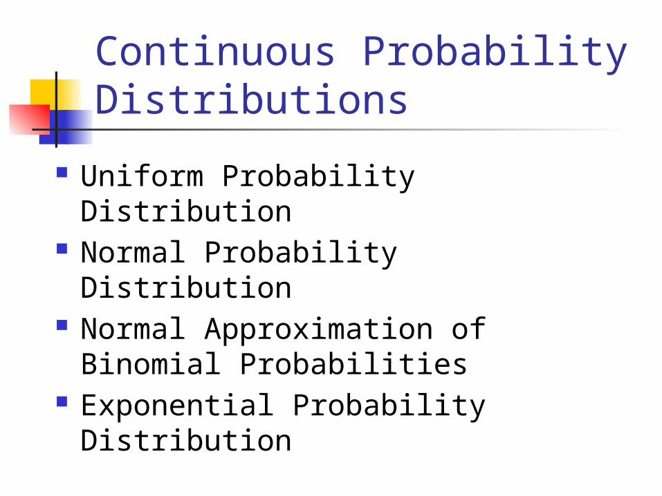
Continuous Probability Distributions
Uniform Probability Distribution Normal Probability Distribution Normal Approximation of Binomial
Probabilities Exponential Probability Distribution
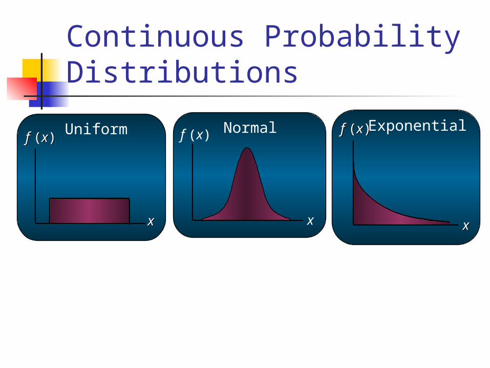
Continuous Probability Distributions
f (x)f (x)
x x
Uniform
x
f (x) Normal
xx
f (x)f (x) Exponential

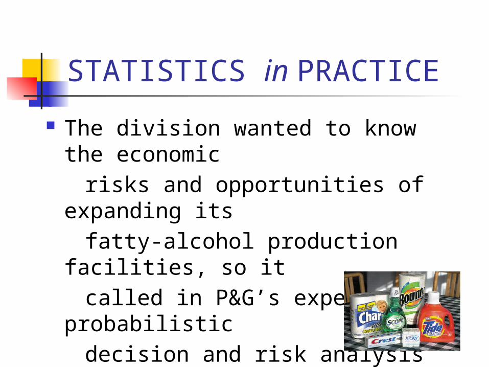
STATISTICS in PRACTICE Procter & Gamble (P&G) produces
and markets such products as
detergents, disposable diapers,
bar soaps, and paper towels. The Industrial Chemicals Division
of P&G is a supplier of fatty alcohols derived from natural substances such as coconut oil and from petroleum- based derivatives.
STATISTICS in PRACTICE
The division wanted to know the economic
risks and opportunities of expanding its
fatty-alcohol production facilities, so it
called in P&G’s experts in probabilistic
decision and risk analysis to help.
Continuous Probability Distributions
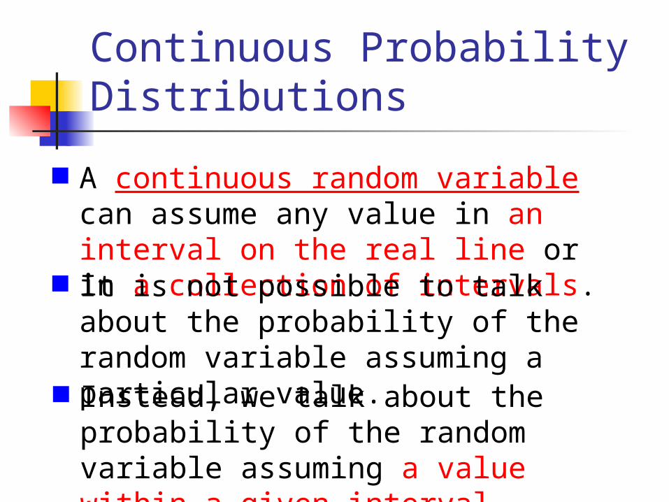
A continuous random variable can assume any value in an interval on the real line or in a collection of intervals.
It is not possible to talk about the probability of the random variable assuming a particular value.
Instead, we talk about the probability of the random variable assuming a value within a given interval.
Continuous Probability Distributions
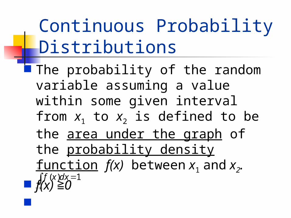
The probability of the random variable assuming a value within some given interval from x1 to x2 is defined to be the area under the graph of the probability density function f(x) between x1 and x2.
f(x) 0≧ 1)(
dxxf
Continuous Probability Distributions
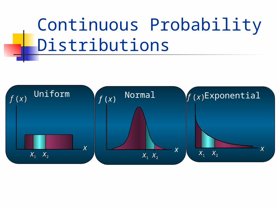
f (x)f (x)
x x
Uniform
x1 x1 x2 x2
x
f (x) Normal
x1 x1 x2 x2 x1 x1 x2 x2
Exponential
xx
f (x)f (x)
x1
x1
x2 x2
Continuous Probability Distributions
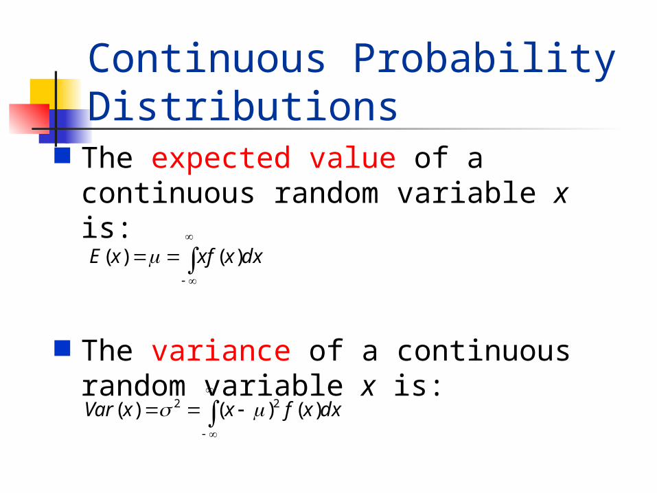
The expected value of a continuous random variable x is:
The variance of a continuous random variable x is:
dxxxfxE )()(
dxxfxxVar )()()( 22
Continuous Probability Distributions
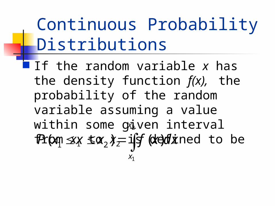
If the random variable x has the density function f(x), the probability of the random variable assuming a value within some given interval from x1 to x2 is defined to be
2
1
)()( 21
x
x
dxxfxxxP
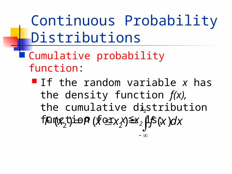
Continuous Probability Distributions
Cumulative probability function: If the random variable x has the density
function f(x), the cumulative distribution function for x x≦ 2 is:
2
)()()( 22
x
dxxfxxPxF
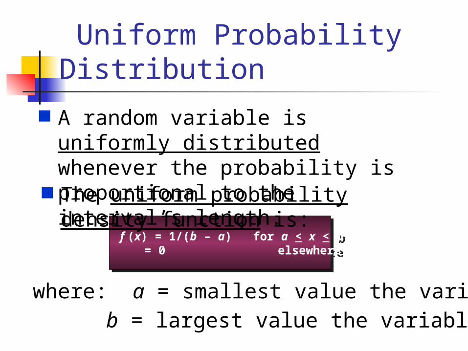
Uniform Probability Distribution
where: a = smallest value the variable can assume
b = largest value the variable can assume
f (x) = 1/(b – a) for a < x < b = 0 elsewhere f (x) = 1/(b – a) for a < x < b = 0 elsewhere
A random variable is uniformly distributed whenever the probability is proportional to the interval’s length.
The uniform probability density function is:
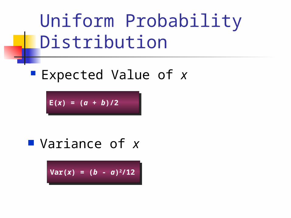
Var(x) = (b - a)2/12Var(x) = (b - a)2/12
E(x) = (a + b)/2E(x) = (a + b)/2
Uniform Probability Distribution
Expected Value of x
Variance of x
Uniform Probability Distribution
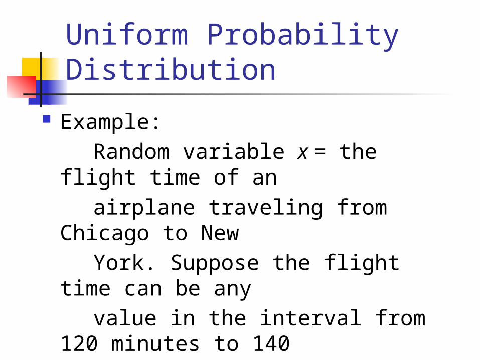
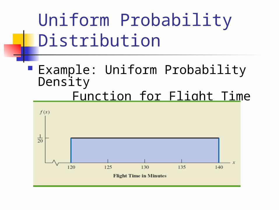
Example:
Random variable x = the flight time of an
airplane traveling from Chicago to New
York. Suppose the flight time can be any
value in the interval from 120 minutes to 140
minutes.
Uniform Probability Distribution
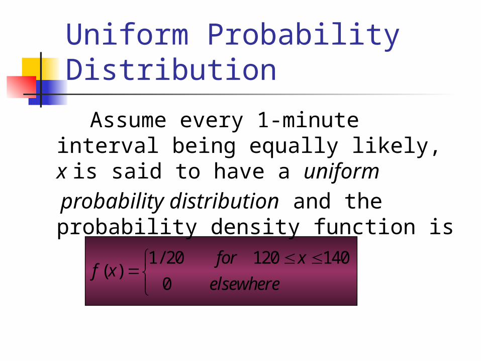
Assume every 1-minute interval being equally likely, x is said to have a uniform
probability distribution and the probability density function is
elsewhere
xforxf
140120
0
20/1)(
Uniform Probability Distribution
Example: Uniform Probability Density Function for Flight Time
Uniform Probability Distribution
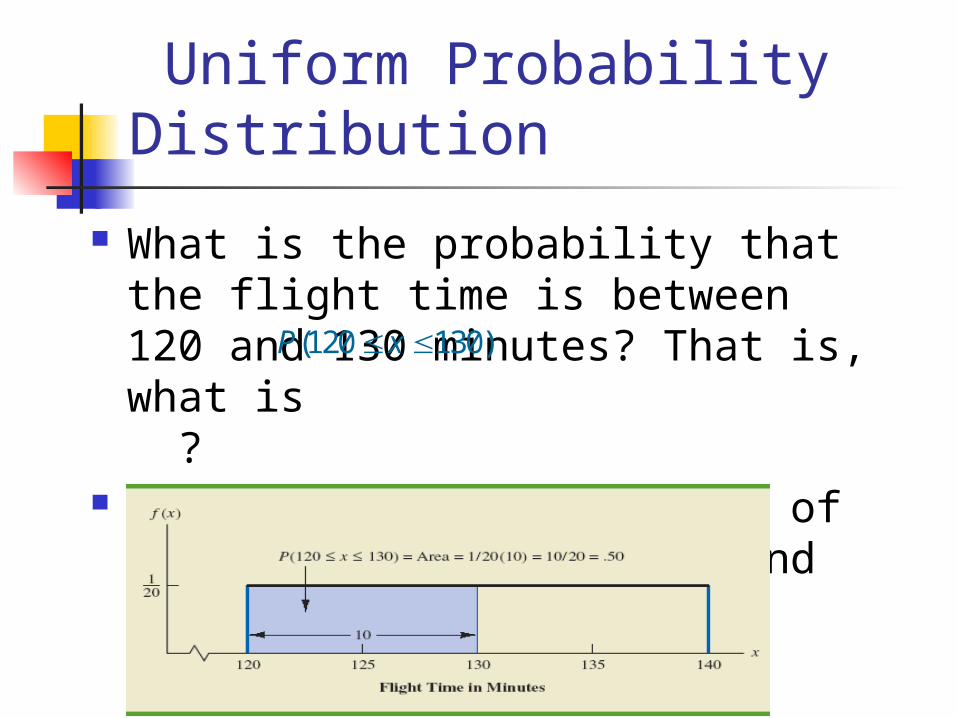
What is the probability that the flight time is between 120 and 130 minutes? That is, what is ?
Area provides Probability of Flight Time Between 120 and 130 Minutes
)130120( xP
Uniform Probability Distribution
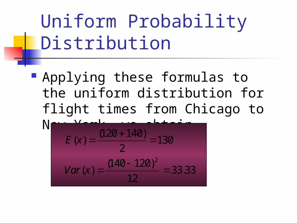
Applying these formulas to the uniform distribution for flight times from Chicago to New York, we obtain
and σ=5.77 minutes.
33.3312
)120140()(
1302
)140120()(
2
xVar
xE
Uniform Probability Distribution
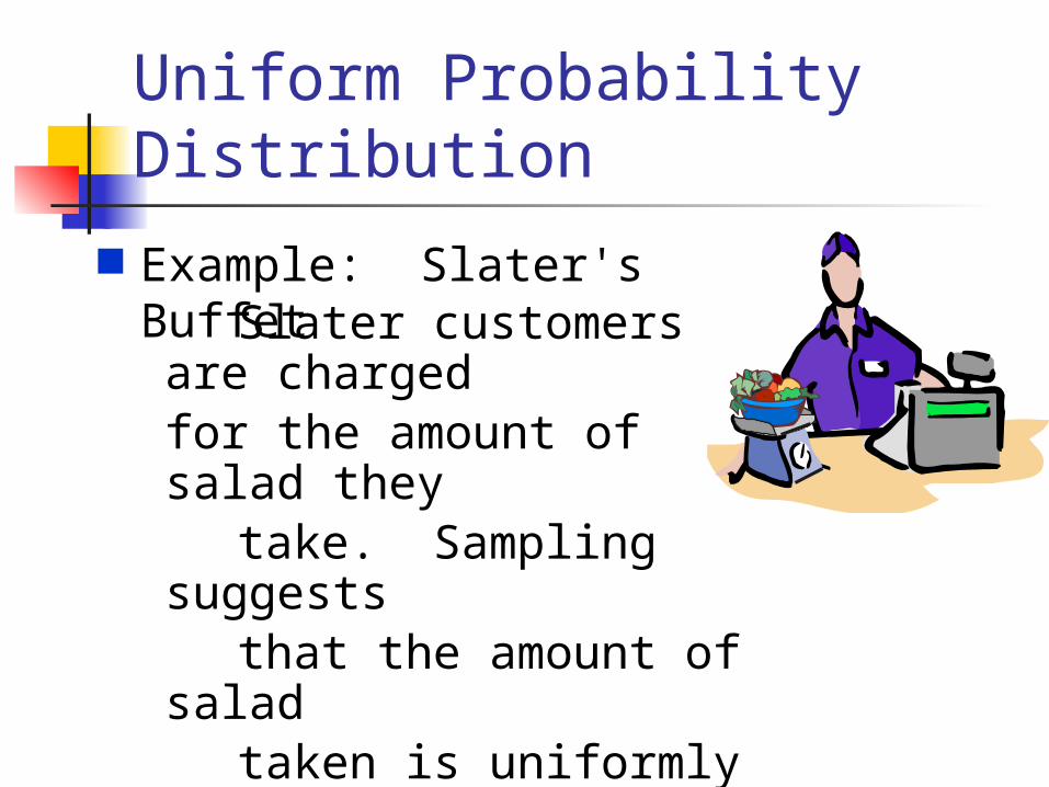
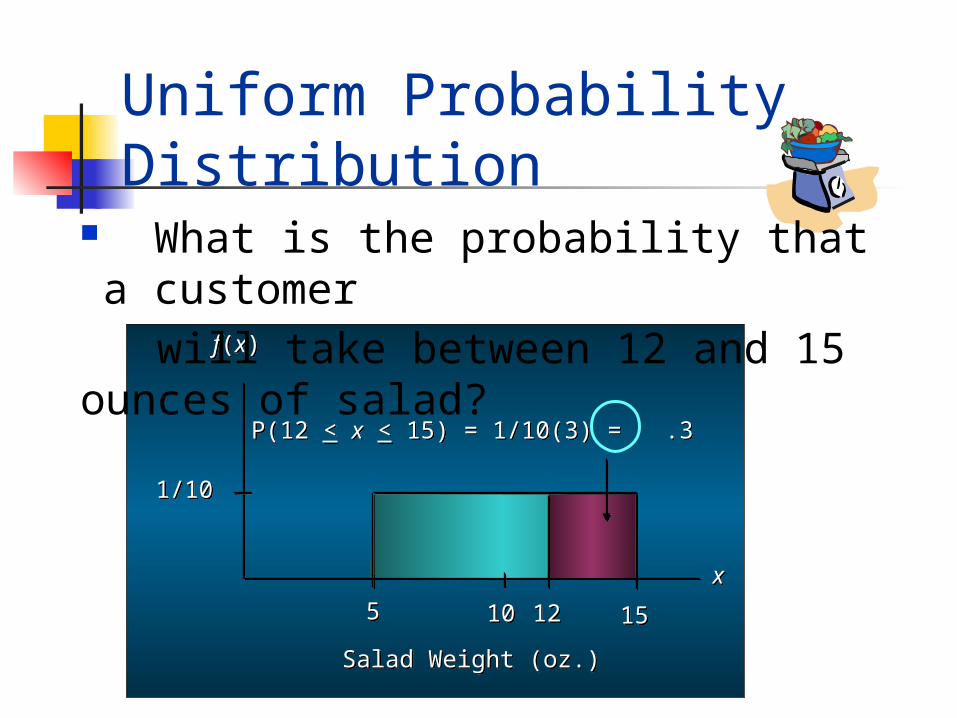
Example: Slater's Buffet Slater customers are charged
for the amount of salad they take. Sampling suggests that the amount of salad taken is uniformly distributed between 5 ounces
and 15 ounces.
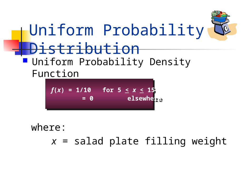
Uniform Probability Density Function
f(x) = 1/10 for 5 < x < 15 = 0 elsewhere
f(x) = 1/10 for 5 < x < 15 = 0 elsewhere
where: x = salad plate filling weight
Uniform Probability Distribution
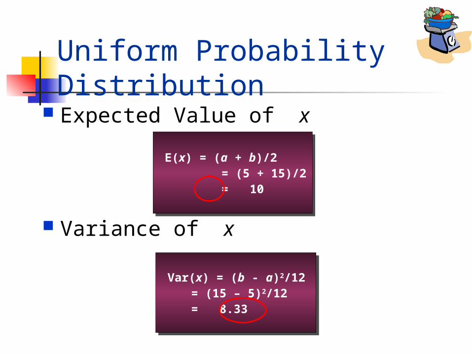
Expected Value of x
Variance of x
E(x) = (a + b)/2 = (5 + 15)/2 = 10
E(x) = (a + b)/2 = (5 + 15)/2 = 10
Var(x) = (b - a)2/12 = (15 – 5)2/12 = 8.33
Var(x) = (b - a)2/12 = (15 – 5)2/12 = 8.33
Uniform Probability Distribution
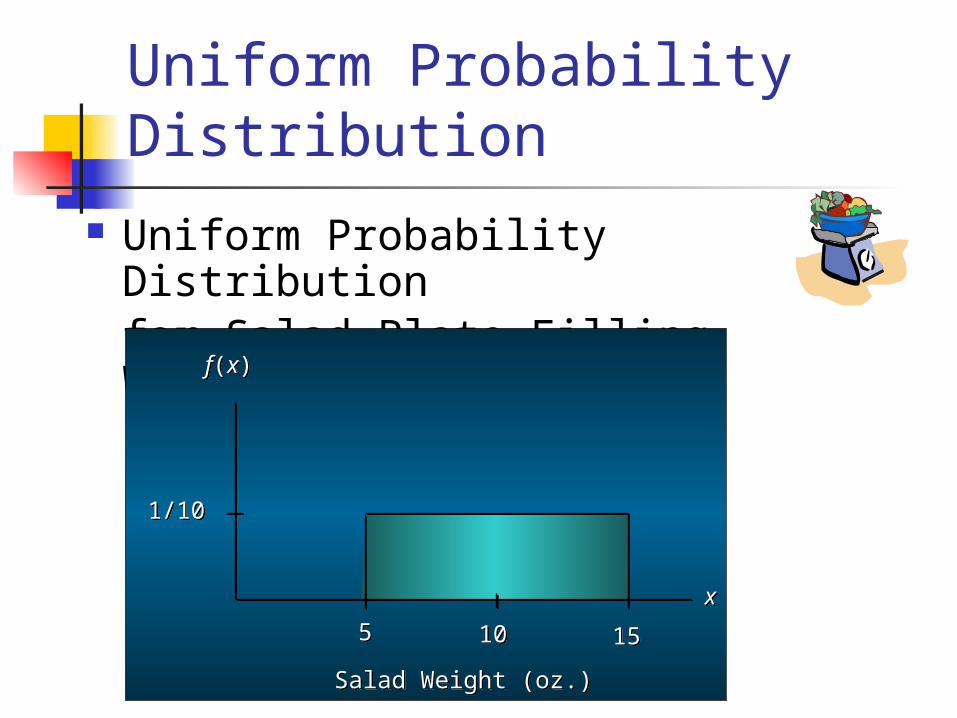
Uniform Probability Distributionfor Salad Plate Filling Weight
f(x)f(x)
x x
55 1010 1515
1/101/10
Salad Weight (oz.)Salad Weight (oz.)
Uniform Probability Distribution
f(x)f(x)
x x
55 1010 1515
1/101/10
Salad Weight (oz.)Salad Weight (oz.)
P(12 < x < 15) = 1/10(3) = .3P(12 < x < 15) = 1/10(3) = .3
What is the probability that a customer
will take between 12 and 15 ounces of salad?
1212
Uniform Probability Distribution
Normal Probability Distribution
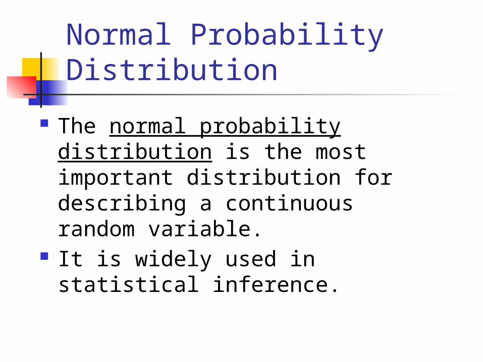
The normal probability distribution is the most important distribution for describing a continuous random variable.
It is widely used in statistical inference.
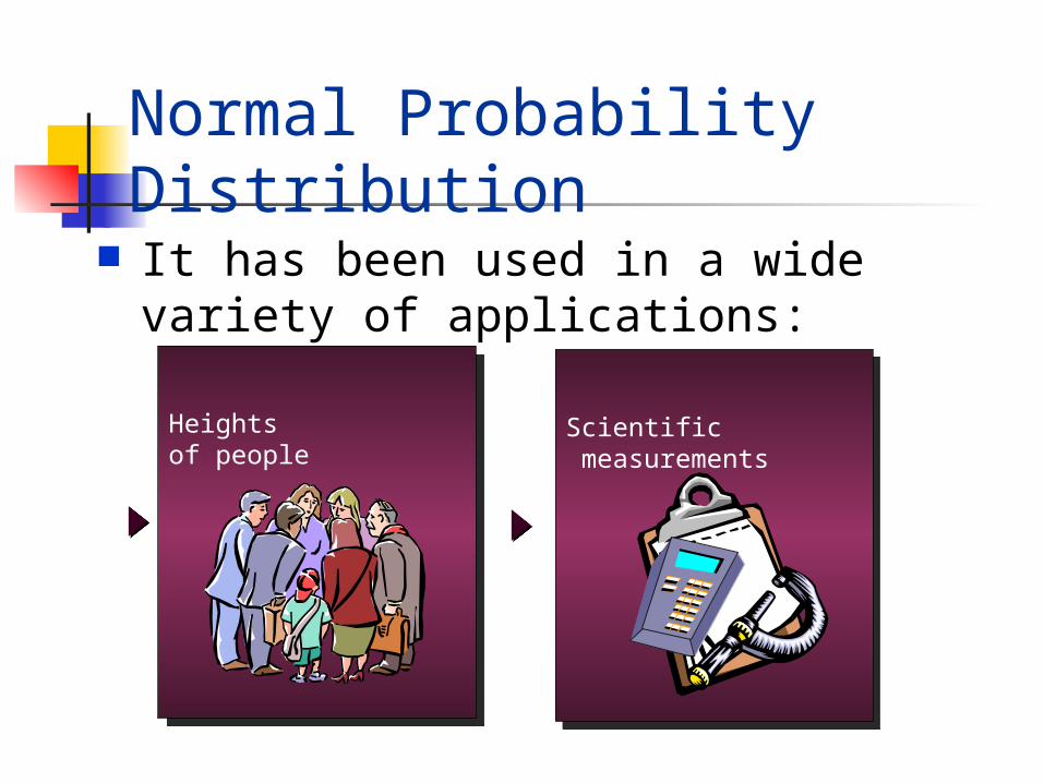
Heightsof people
Heightsof people
Normal Probability Distribution
It has been used in a wide variety of applications:
Scientific measurements
Scientific measurements
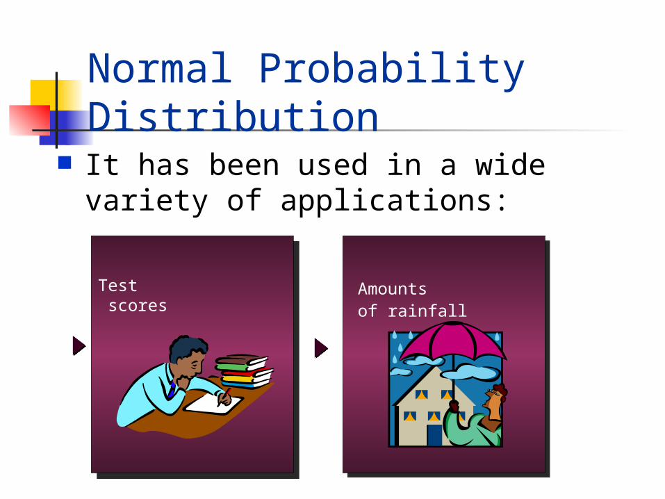
Amountsof rainfall
Amountsof rainfall
Normal Probability Distribution
It has been used in a wide variety of applications:
Test scores
Test scores
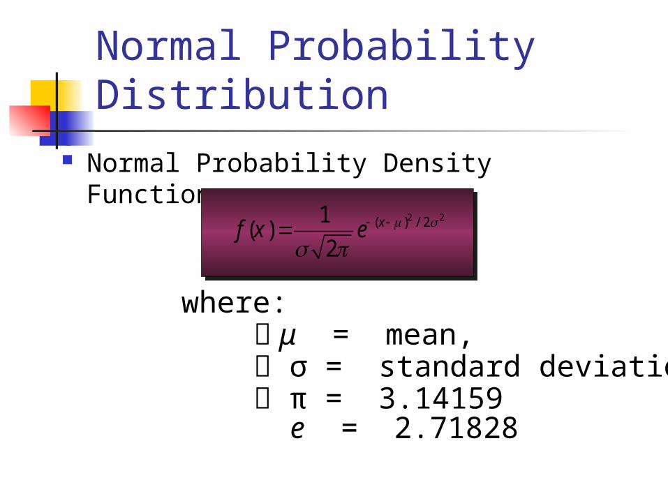
Normal Probability Distribution Normal Probability Density Function
2 2( ) / 21( )
2xf x e
μ = mean, σ = standard deviation, π = 3.14159
e = 2.71828
where:
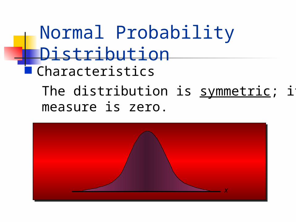
The distribution is symmetric; its skewness measure is zero.
Normal Probability Distribution Characteristics
x
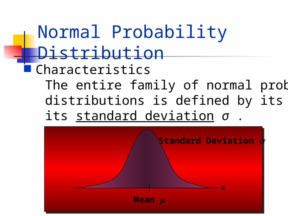
The entire family of normal probability distributions is defined by its mean μ and its standard deviation σ .
Normal Probability Distribution Characteristics
Standard Deviation s
Mean mx
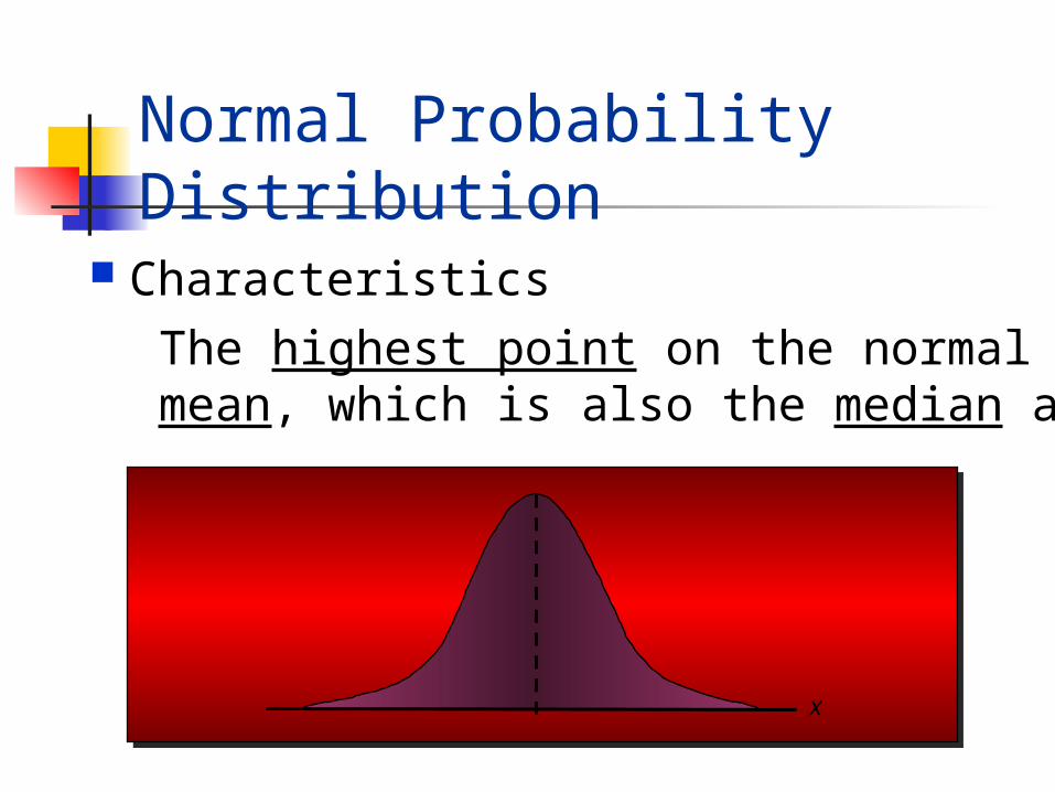
The highest point on the normal curve is at the mean, which is also the median and mode.
Normal Probability Distribution
Characteristics
x
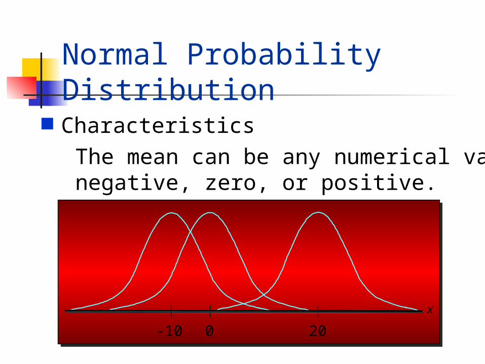
Normal Probability Distribution
Characteristics
-10 0 20
The mean can be any numerical value: negative, zero, or positive.
x
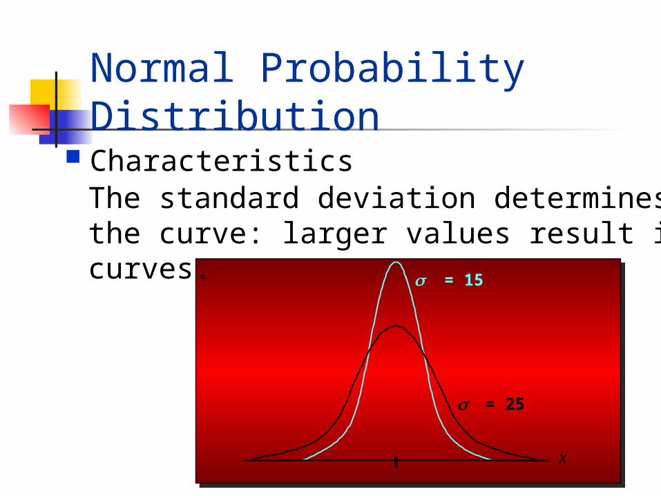
Normal Probability Distribution
Characteristics
s = 15
s = 25
The standard deviation determines the width ofthe curve: larger values result in wider, flatter curves.
x
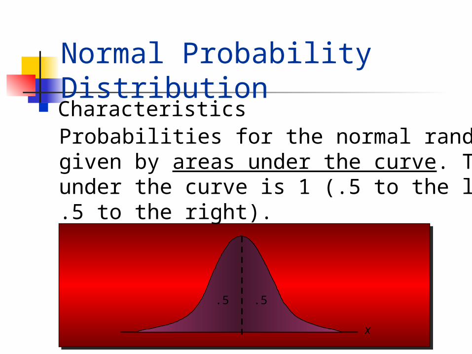
Probabilities for the normal random variable are given by areas under the curve. The total area under the curve is 1 (.5 to the left of the mean and .5 to the right).
Normal Probability Distribution Characteristics
.5 .5
x
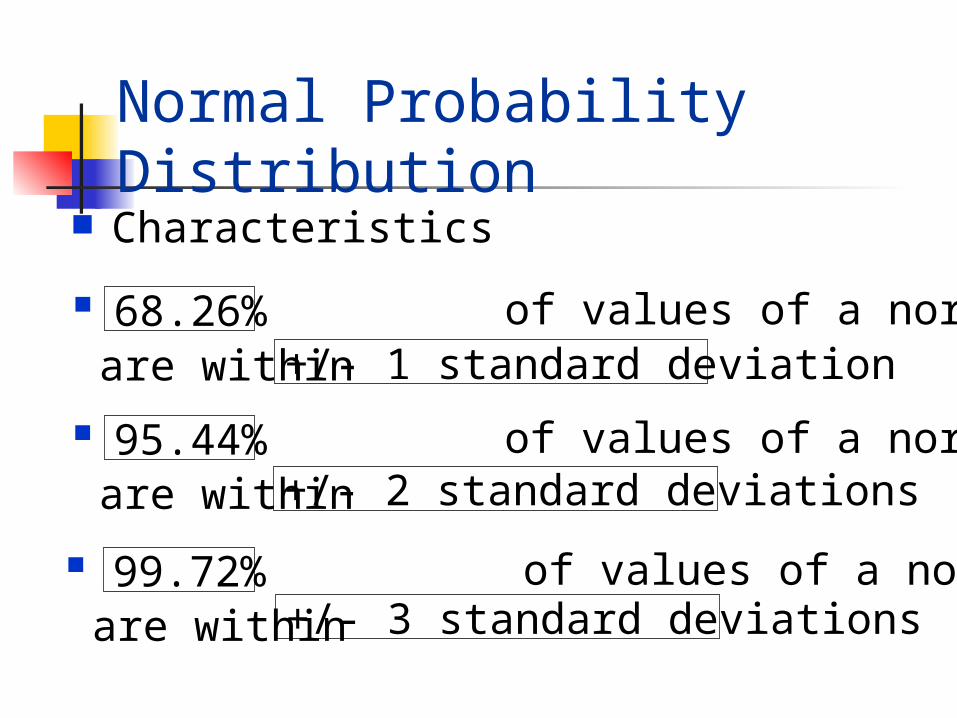
Normal Probability Distribution
of values of a normal random variable are within of its mean.
68.26%+/- 1 standard deviation
of values of a normal random variable are within of its mean.
95.44%+/- 2 standard deviations
of values of a normal random variable are within of its mean.
99.72%+/- 3 standard deviations
Characteristics
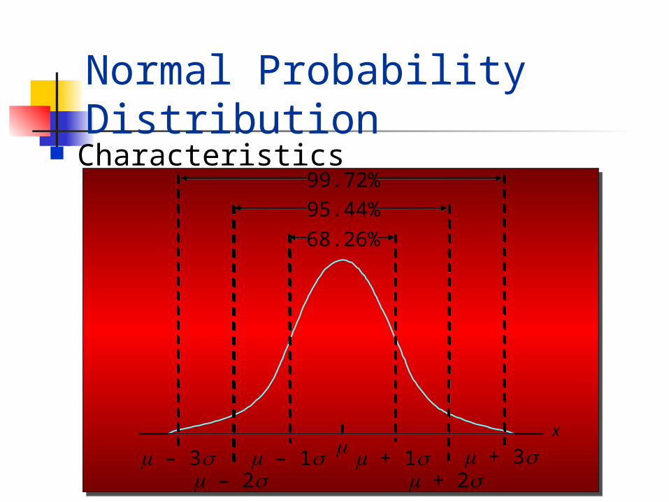
Normal Probability Distribution
x
m – 3s m – 1sm – 2s
m + 1sm + 2s
m + 3sm
68.26%
95.44%99.72%
Characteristics
Standard Normal Probability Distribution
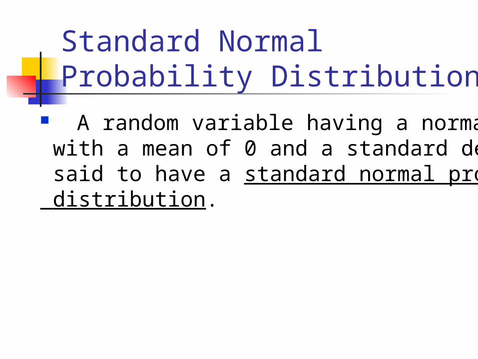
A random variable having a normal distribution with a mean of 0 and a standard deviation of 1 is said to have a standard normal probability distribution.
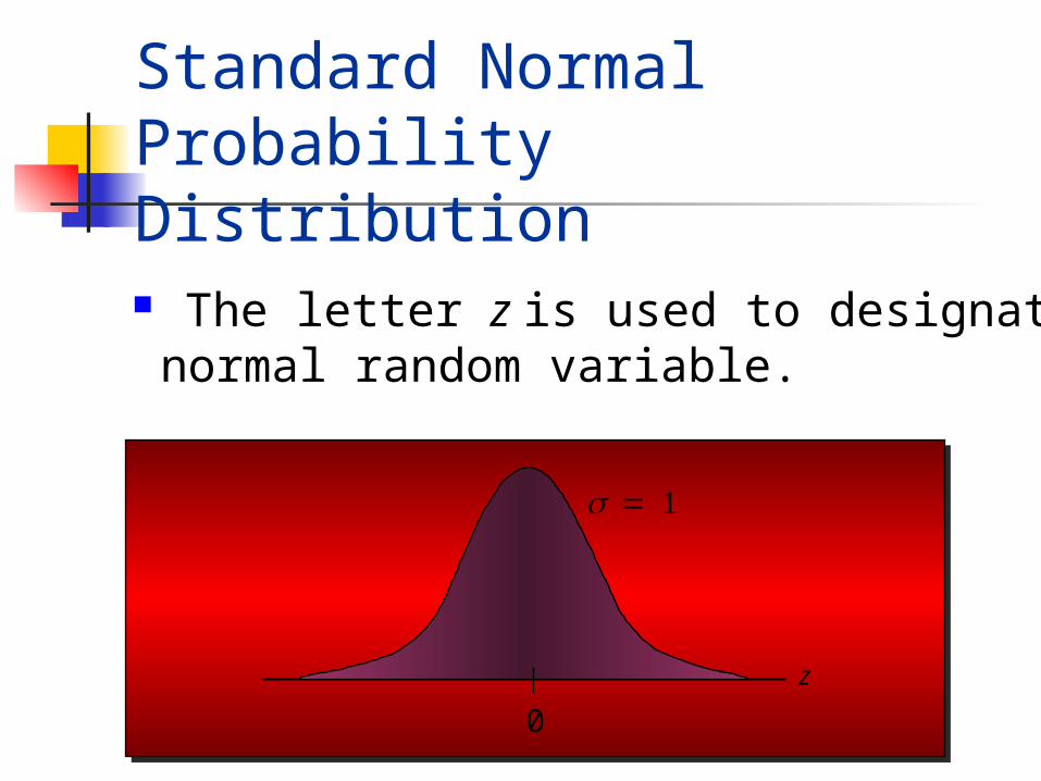
s = 1
0
z
The letter z is used to designate the standard normal random variable.
Standard Normal Probability Distribution

Standard Normal Probability Distribution
Areas, or probabilities, for The Standard Normal Distribution
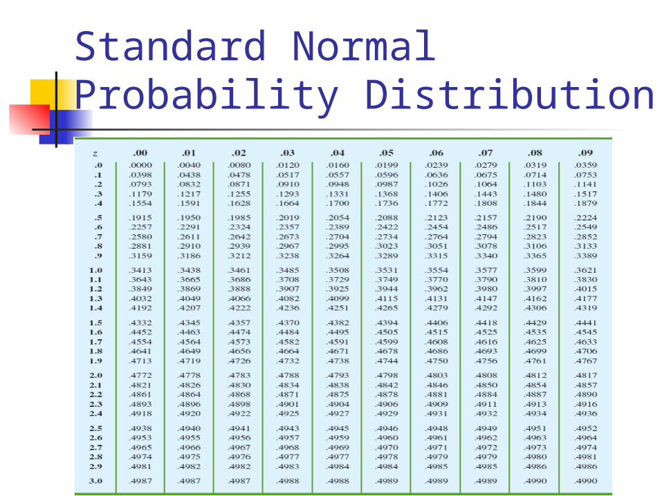
Standard Normal Probability Distribution
Standard Normal Probability Distribution
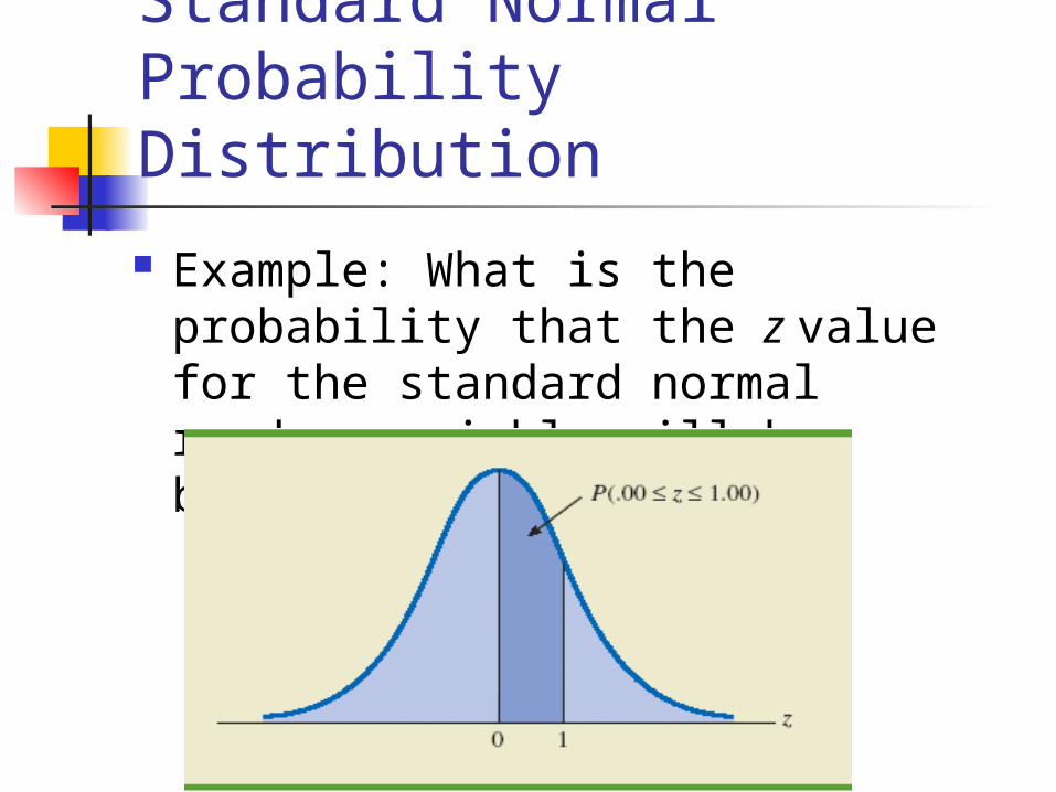
Example: What is the probability that the z value for the standard normal random variable will be between .00 and 1.00?
Standard Normal Probability Distribution
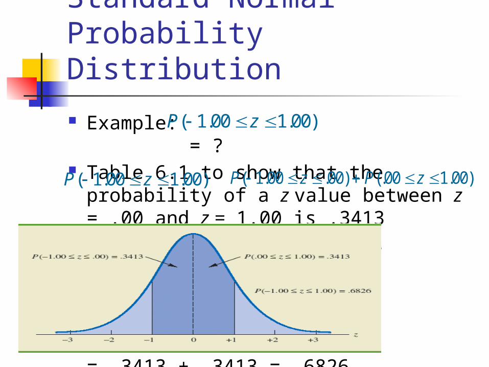
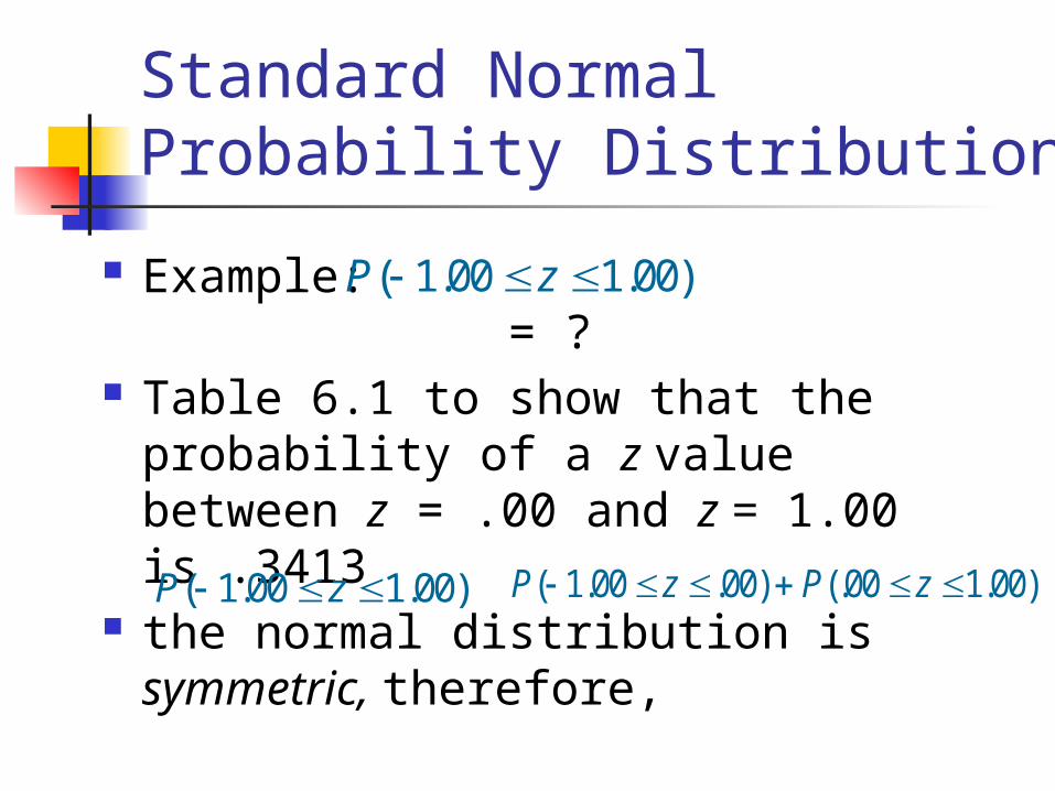
Standard Normal Probability Distribution
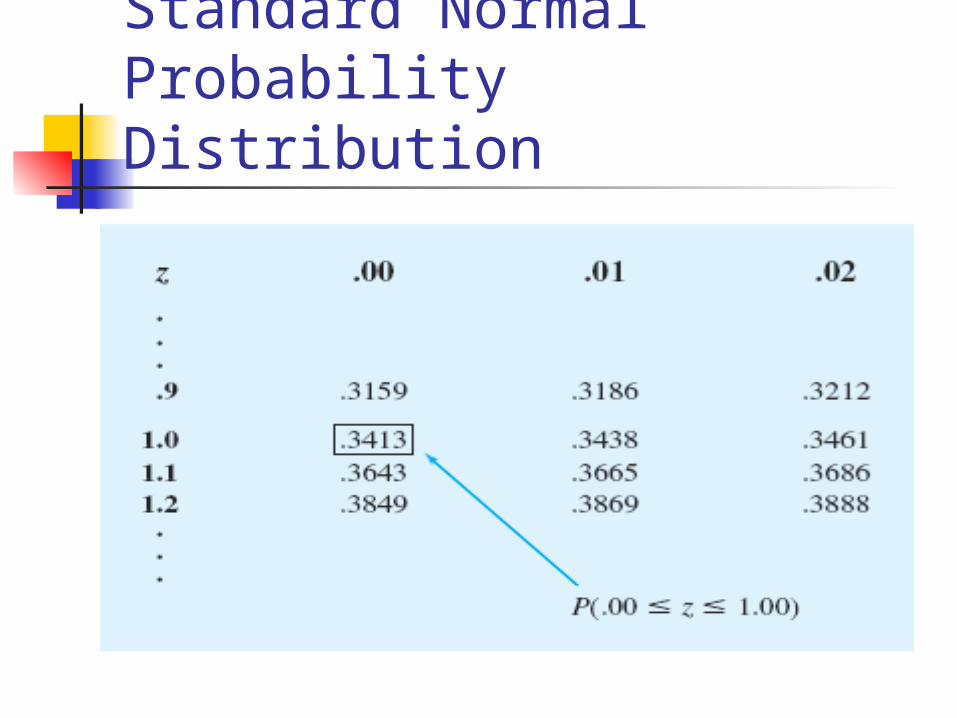
Example: = ? Table 6.1 to show that the probability of a z value
between z = .00 and z = 1.00 is .3413 the normal distribution is symmetric, therefore,
=
= .3413 + .3413 = .6826
)00.100.1( zP
)00.100(.)00.00.1( zPzP)00.100.1( zP
Standard Normal Probability Distribution
Example: = ? Table 6.1 to show that the probability of a z
value between z = .00 and z = 1.00 is .3413 the normal distribution is symmetric,
therefore,
=
= .3413 + .3413 = .6826
)00.100.1( zP
)00.100(.)00.00.1( zPzP)00.100.1( zP
Standard Normal Probability Distribution
Standard Normal Probability Distribution
Example: = ? =
the normal distribution is symmetric and
=
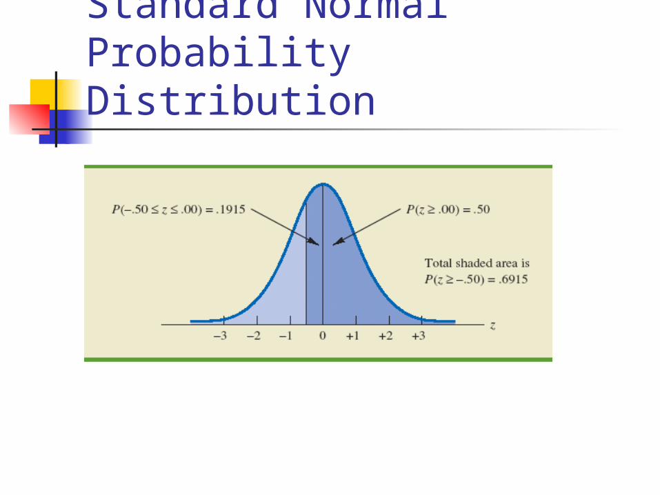
= .1915 + .5000 = .6915.
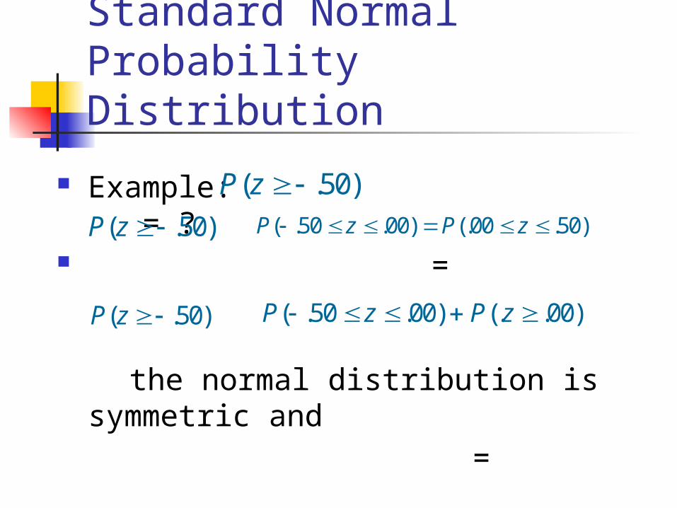
)50.( zP
)50.( zP )00.(.)00.50.( zPzP
)50.00(.)00.50.( zPzP)50.( zP
Standard Normal Probability Distribution

Standard Normal Probability Distribution
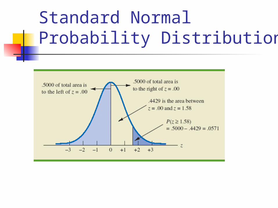
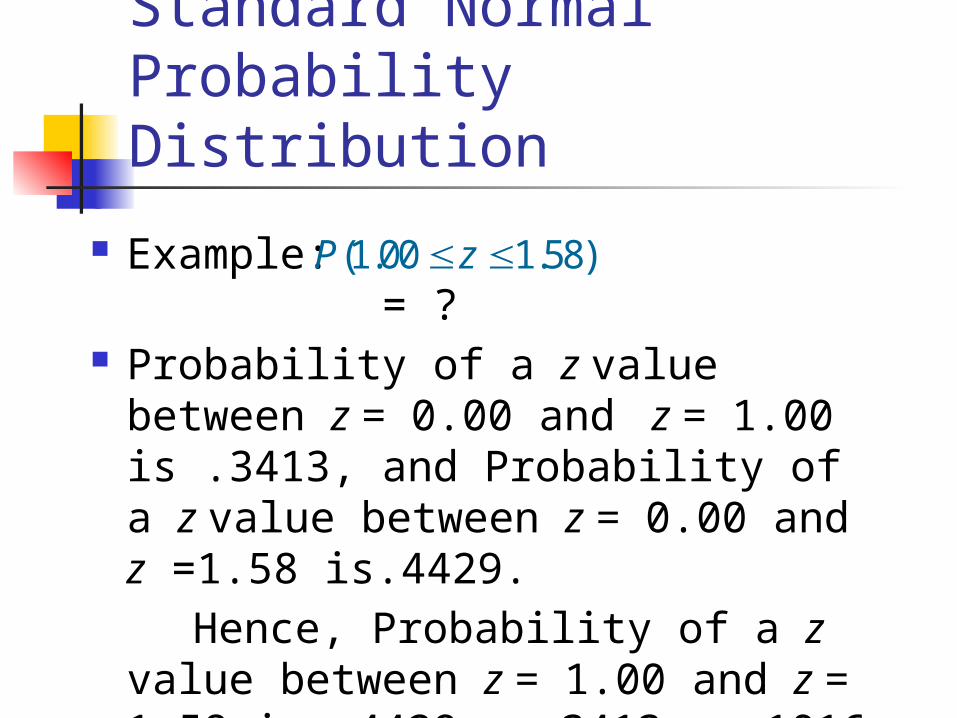
Example: = ? Probability of a z value between z = 0.00 and
z = 1.00 is .3413, and Probability of a z value between z = 0.00 and z =1.58 is .4429 .
Hence, Probability of a z value between z = 1.00 and z = 1.58 is .4429 — .3413 = .1016.
)58.100.1( zP
Standard Normal Probability Distribution
Example: = ? Probability of a z value between z = 0.00
and z = 1.00 is .3413, and Probability of a z value between z = 0.00 and z =1.58 is.4429.
Hence, Probability of a z value between z = 1.00 and z = 1.58 is .4429 — .3413 = .1016
)58.100.1( zP
Standard Normal Probability Distribution
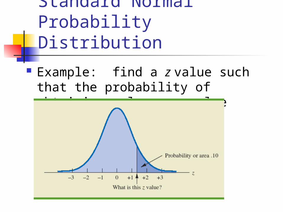
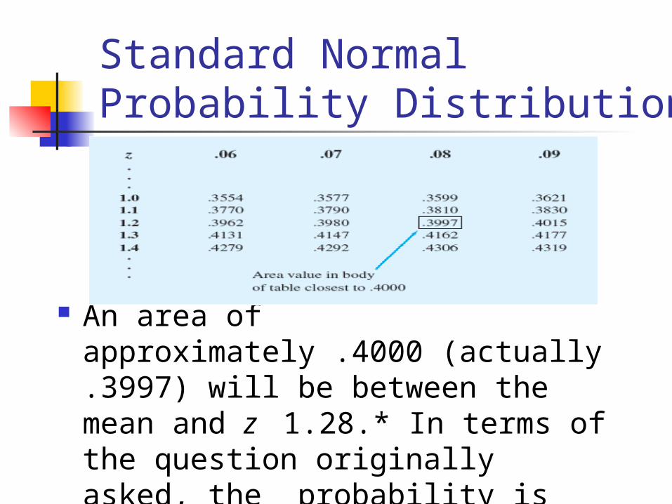
Example: find a z value such that the probability of obtaining a larger z value is .10.
Standard Normal Probability Distribution
An area of approximately .4000 (actually .3997) will be between the mean and z 1.28.* In terms of the question originally asked, the probability is approximately .10 that the z value will be larger than 1.28.
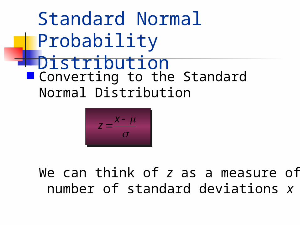
Converting to the Standard Normal Distribution
Standard Normal ProbabilityDistribution
zx
We can think of z as a measure of the number of standard deviations x is from .
Standard Normal Probability Distribution
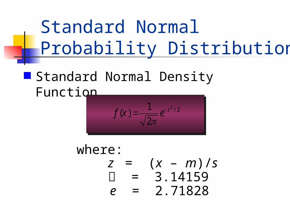
Standard Normal Density Function
2 / 21( )
2zf x e
z = (x – m)/s = 3.14159e = 2.71828
where:
Standard Normal Probability Distribution
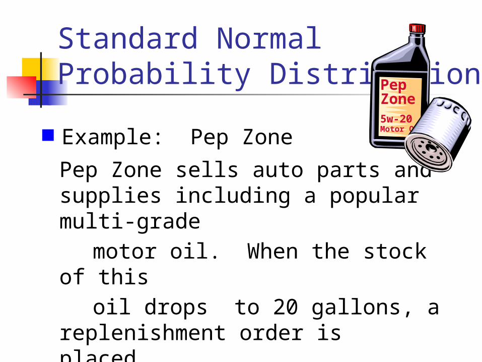
Example: Pep Zone
Pep Zone sells auto parts and supplies including a popular multi-grade
motor oil. When the stock of this
oil drops to 20 gallons, a replenishment order is placed.
PepZone5w-20Motor Oil
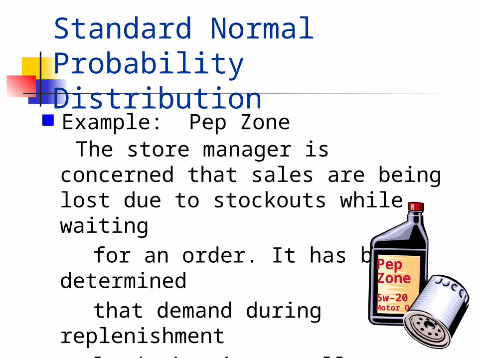
The store manager is concerned that sales are being lost due to stockouts while waiting
for an order. It has been determined
that demand during replenishment
lead-time is normally distributed
with a mean of 15 gallons and a
standard deviation of 6 gallons.
Standard Normal Probability Distribution
PepZone5w-20Motor Oil
Example: Pep Zone
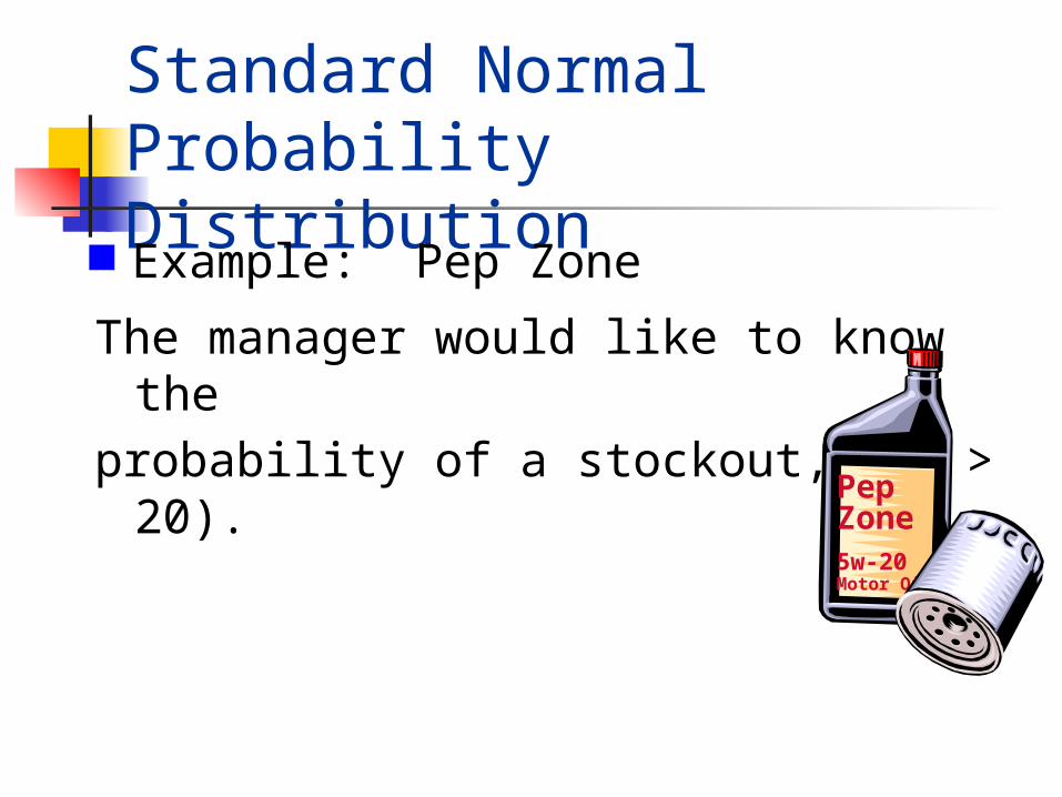
The manager would like to know the
probability of a stockout, P(x > 20).
Standard Normal Probability Distribution
PepZone5w-20Motor Oil
Example: Pep Zone
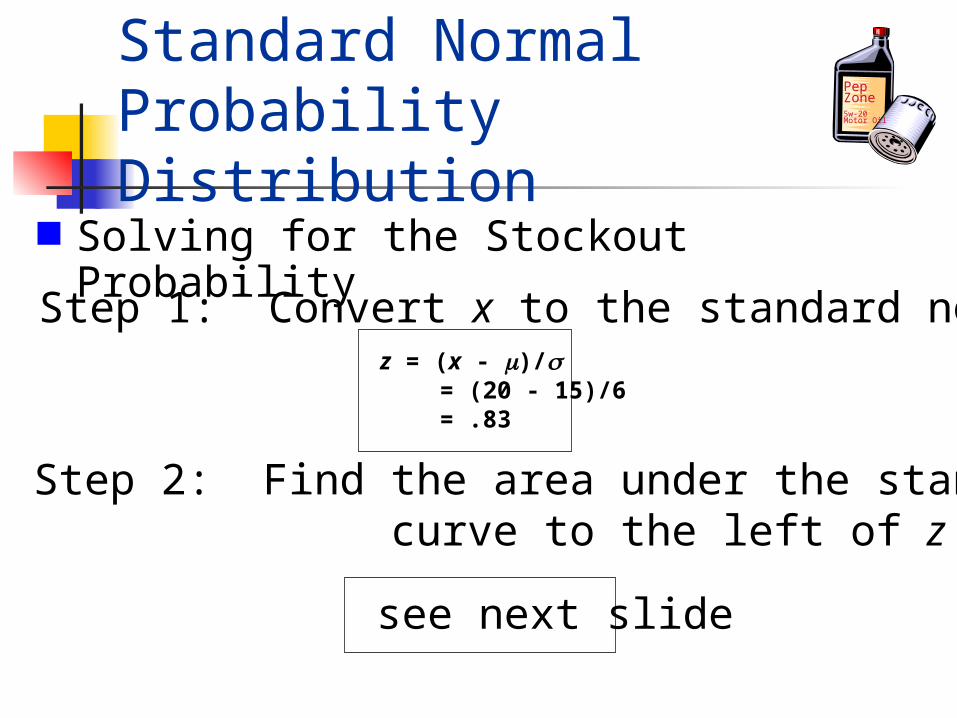
z = (x - )/ = (20 - 15)/6 = .83
Solving for the Stockout Probability
Step 1: Convert x to the standard normal distribution.
PepZone5w-20Motor Oil
Step 2: Find the area under the standard normal curve to the left of z = .83.
see next slide
Standard Normal Probability Distribution
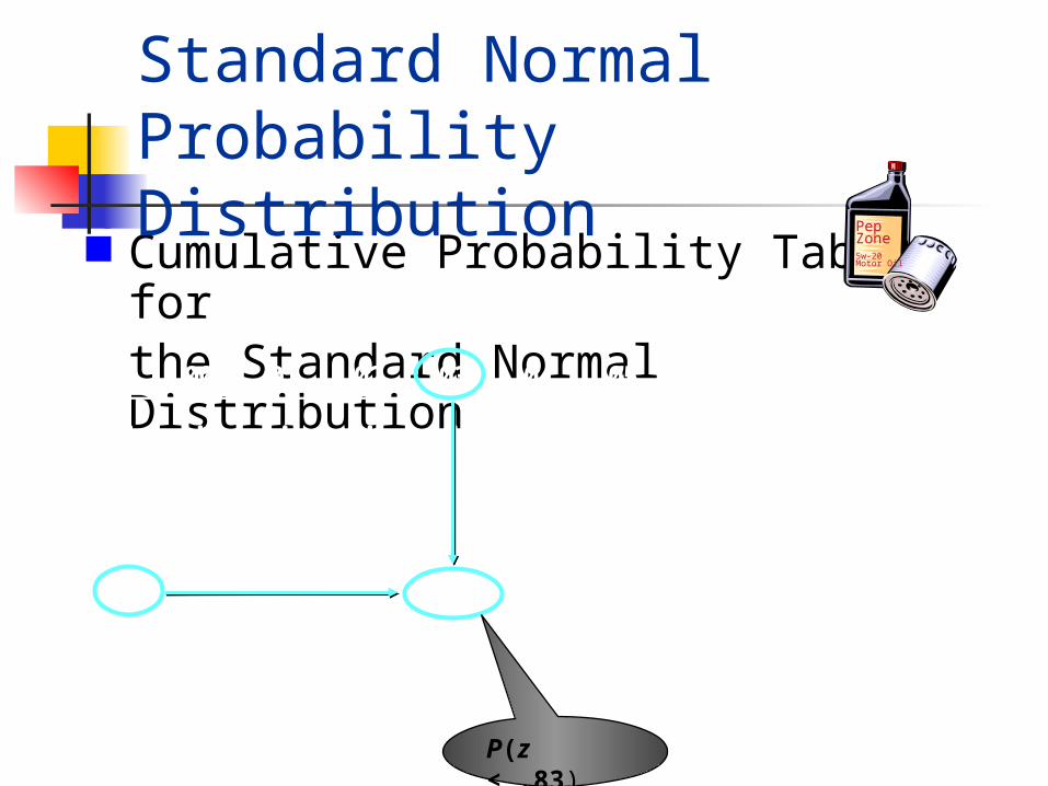
Cumulative Probability Table for the Standard Normal Distributionz .00 .01 .02 .03 .04 .05 .06 .07 .08 .09
. . . . . . . . . . .
.5 .6915 .6950 .6985 .7019 .7054 .7088 .7123 .7157 .7190 .7224
.6 .7257 .7291 .7324 .7357 .7389 .7422 .7454 .7486 .7517 .7549
.7 .7580 .7611 .7642 .7673 .7704 .7734 .7764 .7794 .7823 .7852
.8 .7881 .7910 .7939 .7967 .7995 .8023 .8051 .8078 .8106 .8133
.9 .8159 .8186 .8212 .8238 .8264 .8289 .8315 .8340 .8365 .8389
. . . . . . . . . . .
PepZone5w-20Motor Oil
P(z < .83)
Standard Normal Probability Distribution
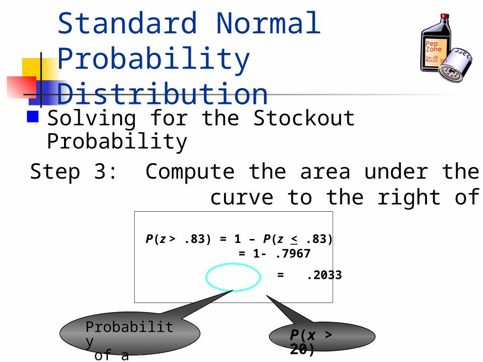
P(z > .83) = 1 – P(z < .83) = 1- .7967
= .2033
Solving for the Stockout Probability
Step 3: Compute the area under the standard normal curve to the right of z = .83.
PepZone5w-20Motor Oil
Probability of a stockout P(x >
20)
Standard Normal Probability Distribution
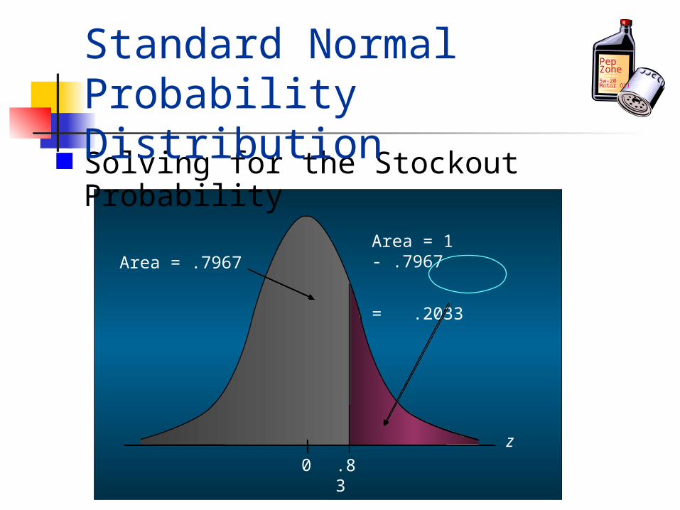
Solving for the Stockout Probability
0 .83
Area = .7967Area = 1 - .7967
= .2033
z
PepZone5w-20Motor Oil
Standard Normal Probability Distribution
Standard Normal Probability Distribution
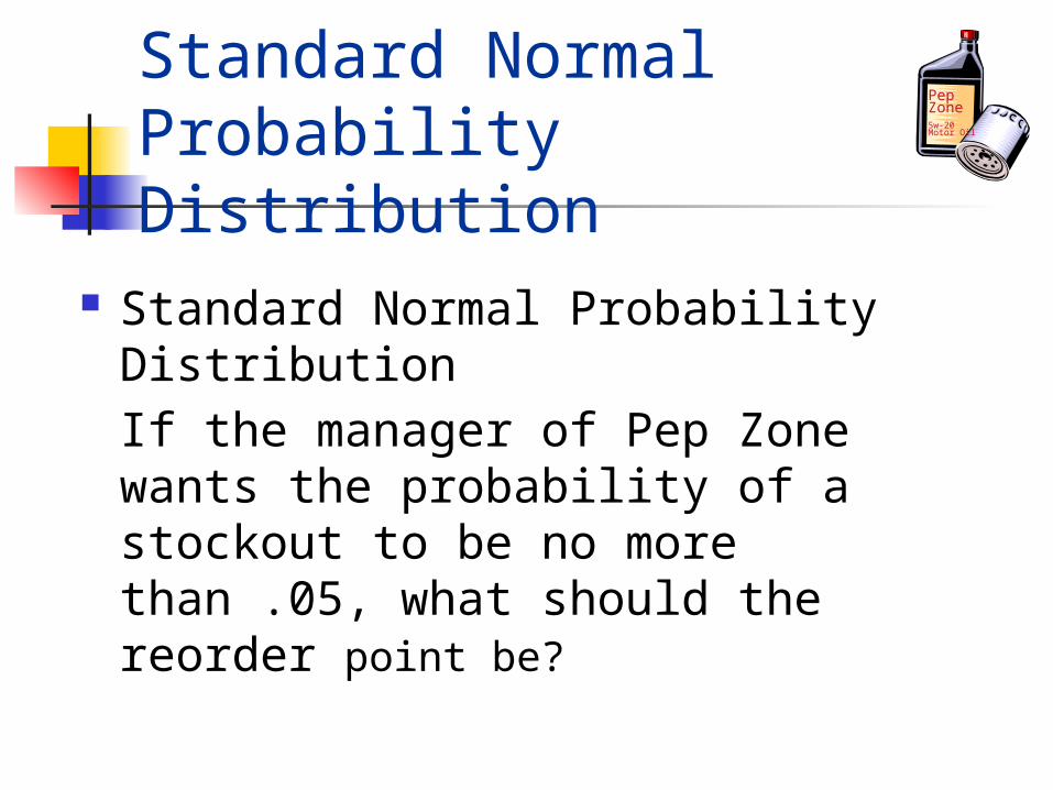
If the manager of Pep Zone wants the probability of a stockout to be no more than .05, what should the reorder point be?
PepZone5w-20Motor Oil
Standard Normal Probability Distribution
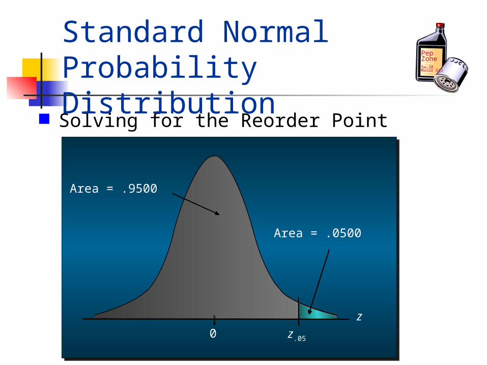
Solving for the Reorder Point
PepZone5w-20Motor Oil
0
Area = .9500
Area = .0500
zz.05
Standard Normal Probability Distribution

Solving for the Reorder Point
PepZone5w-20Motor Oil
Step 1: Find the z-value that cuts off an area of .05 in the right tail of the standard normal distribution.
z .00 .01 .02 .03 .04 .05 .06 .07 .08 .09
. . . . . . . . . . .
1.5 .9332 .9345 .9357 .9370 .9382 .9394 .9406 .9418 .9429 .9441
1.6 .9452 .9463 .9474 .9484 .9495 .9505 .9515 .9525 .9535 .9545
1.7 .9554 .9564 .9573 .9582 .9591 .9599 .9608 .9616 .9625 .9633
1.8 .9641 .9649 .9656 .9664 .9671 .9678 .9686 .9693 .9699 .9706
1.9 .9713 .9719 .9726 .9732 .9738 .9744 .9750 .9756 .9761 .9767
. . . . . . . . . . .We look up the complement of the tail area (1 - .05 = .95)
Standard Normal Probability Distribution
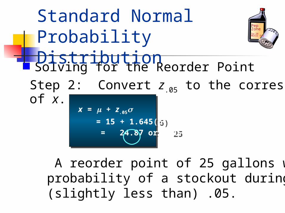
Solving for the Reorder Point
PepZone5w-20Motor Oil
Step 2: Convert z.05 to the corresponding value of x.
x = + z.05 = 15 + 1.645(6) = 24.87 or 25
x = + z.05 = 15 + 1.645(6) = 24.87 or 25
A reorder point of 25 gallons will place the probability of a stockout during leadtime at (slightly less than) .05.
Standard Normal Probability Distribution
Solving for the Reorder Point
PepZone5w-20Motor Oil
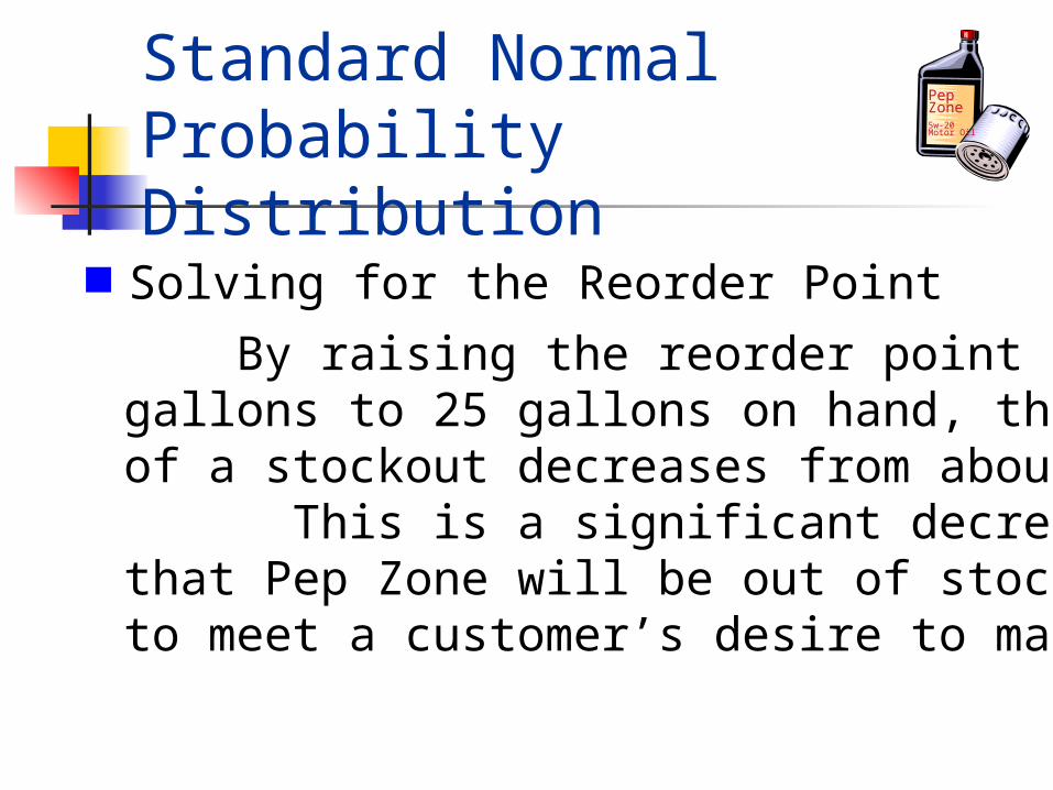
By raising the reorder point from 20 gallons to 25 gallons on hand, the probability of a stockout decreases from about .20 to .05. This is a significant decrease in the chance that Pep Zone will be out of stock and unable to meet a customer’s desire to make a purchase.
Standard Normal Probability Distribution
Normal Approximation of Binomial Probabilities
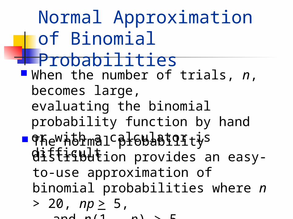
When the number of trials, n, becomes large,evaluating the binomial probability function by hand or with a calculator is difficult
The normal probability distribution provides an easy-to-use approximation of binomial probabilities where n > 20, np > 5,
and n(1 - p) > 5.
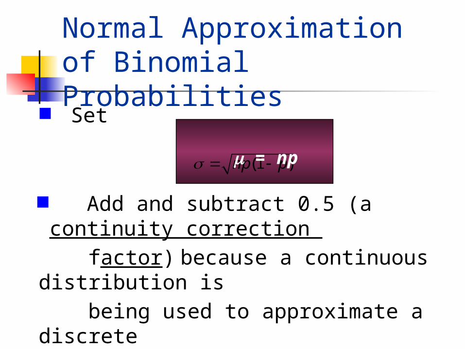
Normal Approximation of Binomial Probabilities
Add and subtract 0.5 (a continuity correction
factor) because a continuous distribution is
being used to approximate a discrete
distribution. For example,
P(x = 10) is approximated by P(9.5 < x < 10.5).
Set
(1 )np p
= np
Normal Approximation of Binomial Probabilities
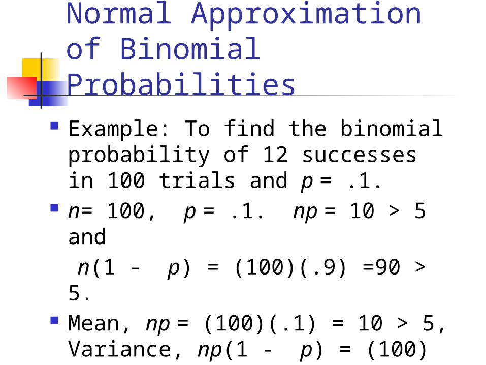
Example: To find the binomial probability of 12 successes in 100 trials and p = .1.
n= 100, p = .1. np = 10 > 5 and
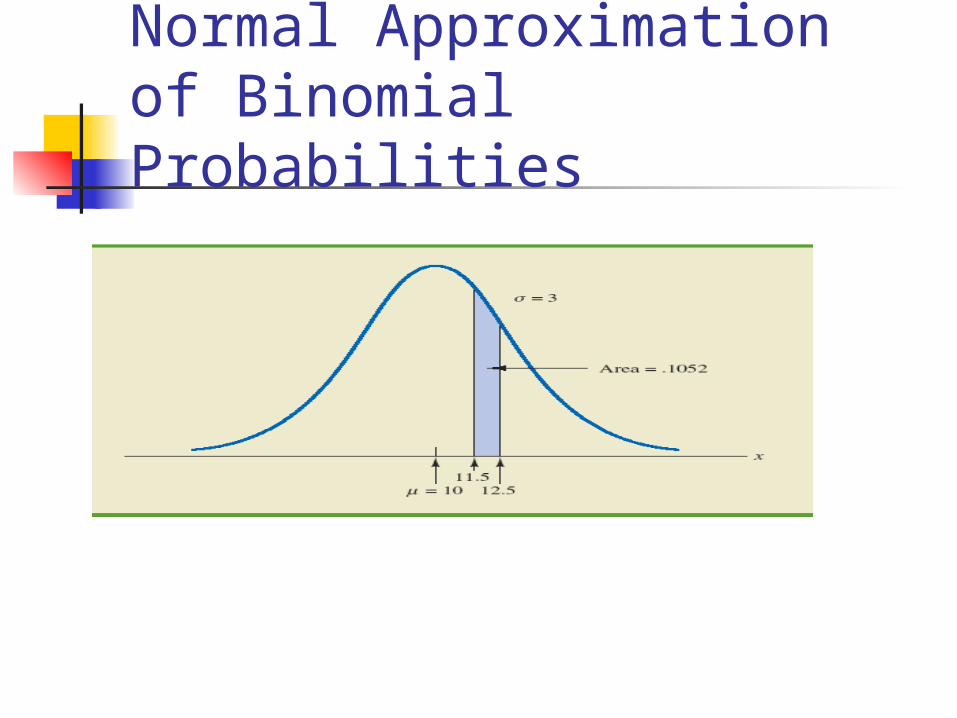
n(1 - p) = (100)(.9) =90 > 5. Mean, np = (100)(.1) = 10 > 5, Variance,
np(1 - p) = (100)(.1)(.9) =9. Compute the area under the corresponding normal curve between 11.5 and 12.5.
Normal Approximation of Binomial Probabilities
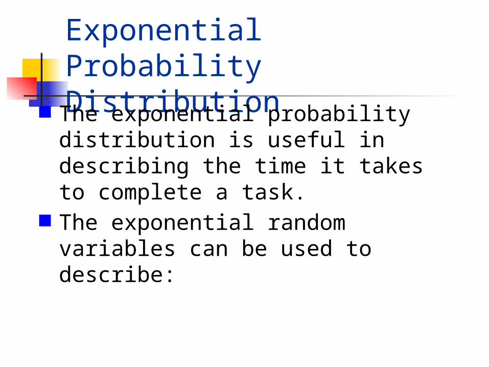
Exponential Probability Distribution
The exponential probability distribution is useful in describing the time it takes to complete a task.
The exponential random variables can be used to describe:
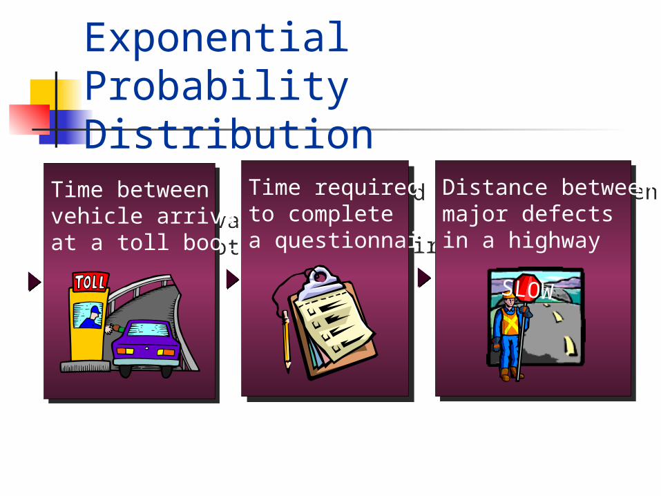
Exponential Probability Distribution
Time betweenvehicle arrivalsat a toll booth
Time betweenvehicle arrivalsat a toll booth
Time requiredto completea questionnaire
Time requiredto completea questionnaire
Distance betweenmajor defectsin a highway
Distance betweenmajor defectsin a highway
SLOW
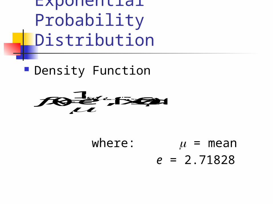
Density Function
Exponential Probability Distribution
where: = mean
e = 2.71828
0 0,xfor ,1
)( /
xexffor x > 0, > 0
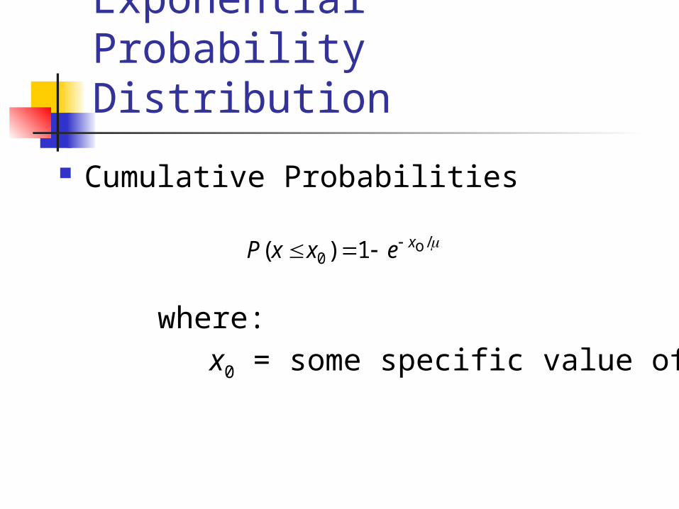
Cumulative Probabilities
Exponential Probability Distribution
P x x e x( ) / 0 1 o
where:
x0 = some specific value of x
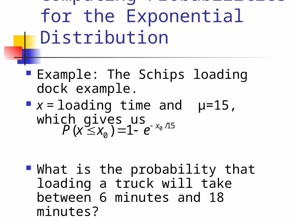
Computing Probabilities for the Exponential Distribution
Example: The Schips loading dock example.
x = loading time and μ=15, which gives us
What is the probability that loading a truck will take between 6 minutes and 18 minutes?
15/0
01)( xexxP
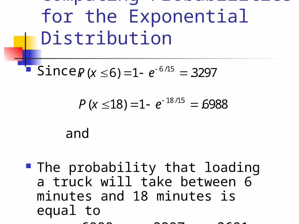
Computing Probabilities for the Exponential Distribution
Since, and The probability that loading a truck will
take between 6 minutes and 18 minutes is equal to
.6988 -- .3297 = .3691.
3297.1)6( 15/6 exP
6988.1)18( 15/18 exP
Exponential Probability Distribution
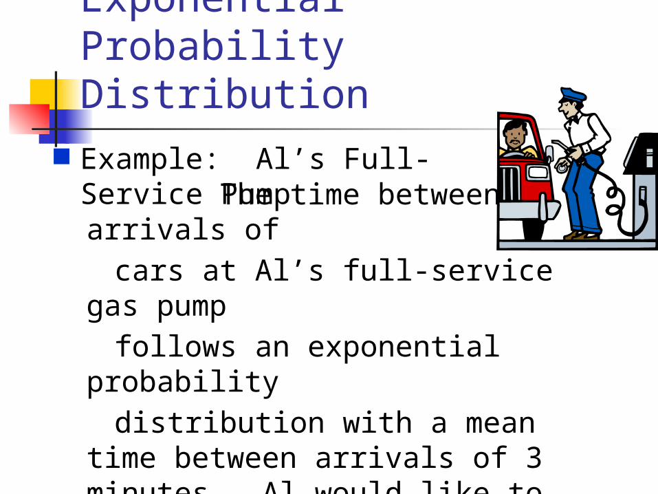
Example: Al’s Full-Service Pump
The time between arrivals of
cars at Al’s full-service gas pump
follows an exponential probability
distribution with a mean time between arrivals of 3 minutes. Al would like to know theprobability that the time between two successive arrivals will be 2 minutes or less.
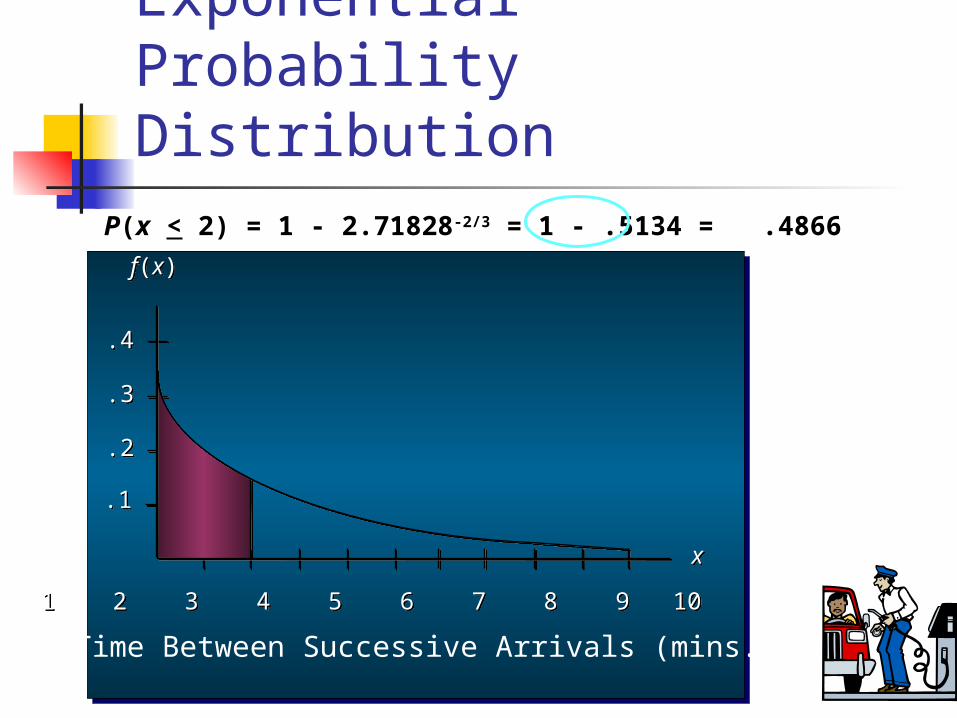
xx
f(x)f(x)
.1.1
.3.3
.4.4
.2.2
1 2 3 4 5 6 7 8 9 10 1 2 3 4 5 6 7 8 9 10
Time Between Successive Arrivals (mins.)
Exponential Probability Distribution
P(x < 2) = 1 - 2.71828-2/3 = 1 - .5134 = .4866
Exponential Probability Distribution
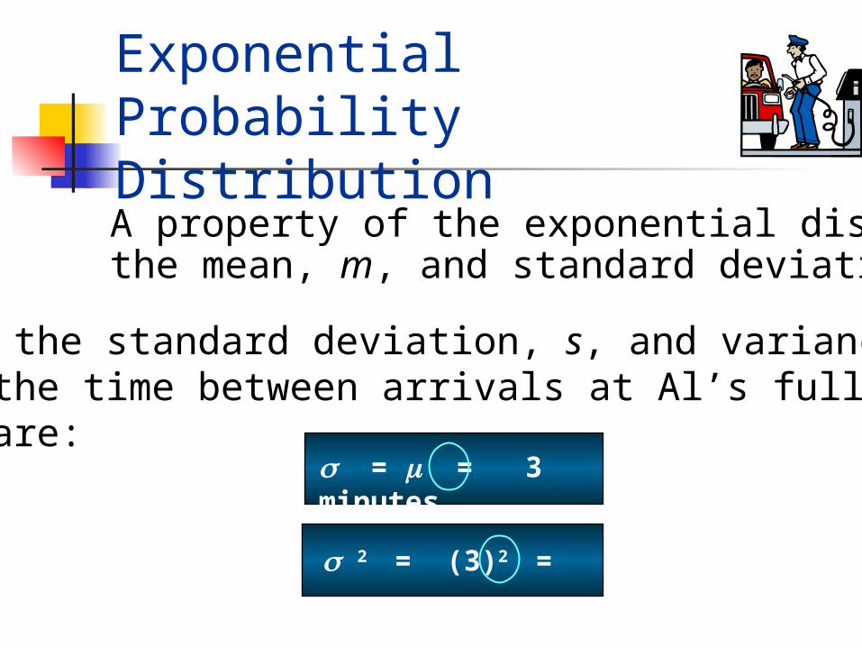
A property of the exponential distribution is that the mean, m, and standard deviation, s, are equal.
Thus, the standard deviation, s, and variance, s 2,for the time between arrivals at Al’s full-service pump are:
s = m = 3 minutes
s 2 = (3)2 = 9
Exponential Probability Distribution
The exponential distribution is skewed to the right.
The skewness measure for the exponential distribution is 2.
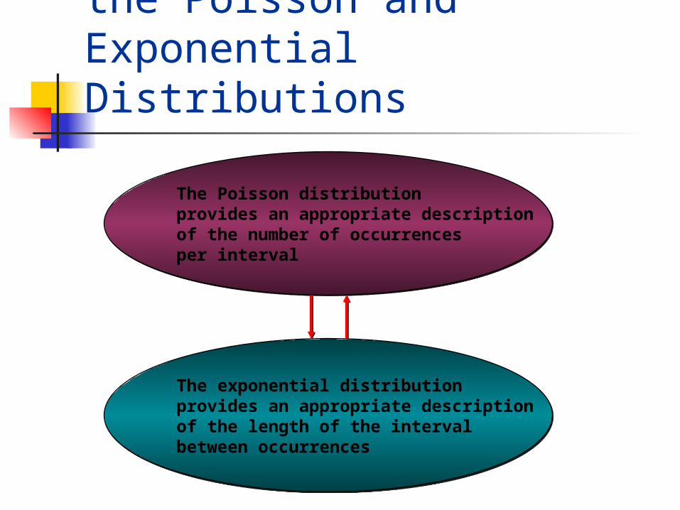
Relationship between the Poisson and Exponential Distributions
The Poisson distributionprovides an appropriate descriptionof the number of occurrencesper interval
The Poisson distributionprovides an appropriate descriptionof the number of occurrencesper interval
The exponential distributionprovides an appropriate descriptionof the length of the intervalbetween occurrences
The exponential distributionprovides an appropriate descriptionof the length of the intervalbetween occurrences