18, N. 2 (2017), 253-272 Tema

�

�

“main” — 2017/8/14 — 12:57 — page 253 — #1�

�

�

�

�

�

TemaTendencias em Matematica Aplicada e Computacional, 18, N. 2 (2017), 253-272© 2017 Sociedade Brasileira de Matematica Aplicada e Computacionalwww.scielo.br/temadoi: 10.5540/tema.2017.018.02.0253

A General Boundary Condition with Linear Fluxfor Advection-Diffusion Models†

T.Y. MIYAOKA1*, J.F.C.A. MEYER1 and J.M.R. SOUZA2

Received on November 21, 2016 / Accepted on April 19, 2017

ABSTRACT. Advection-diffusion equations are widely used in modeling a diverse range of problems.These mathematical models consist in a partial differential equation or system with initial and boundaryconditions, which depend on the phenomena being studied. In the modeling, boundary conditions may beneglected and unnecessarily simplified, or even misunderstood, causing a model not to reflect the realityadequately, making qualitative and/or quantitative analyses more difficult. In this work we derive a generallinear flux dependent boundary condition for advection-diffusion problems and show that it generates allpossible boundary conditions, according to the outward flux on the boundary. This is done through an inte-gral formulation, analyzing the total mass of the system. We illustrate the exposed cases with applicationswilling to clarify their meanings. Numerical simulations, by means of the Finite Difference Method, areused in order to exemplify the different boundary conditions’ impact, making it possible to quantify the fluxalong the boundary. With qualitative and quantitative analysis, this work can be useful to researchers andstudents working on mathematical models with advection-diffusion equations.

Keywords: boundary conditions, partial differential equations, mathematical models, computer simula-tion.

1 INTRODUCTION

The first application of the diffusion equation was done by Fourier in 1822 [1], when he proposedits use to model heat distribution. At that time, the main concern was to analyze the model forsimple cases, including simple boundary conditions such as fixed concentrations at the bound-aries. Once theory was developed, the diffusion equation can now be combined with advection

(or convection) processes, resulting in advection-diffusion equations, which demand more elab-orate boundary conditions, depending on the phenomena being modeled.

†This work was supported by CAPES.*Corresponding author: Tiago Yuzo Miyaoka – E-mail: [email protected] de Matematica Aplicada, IMECC, Universidade Estadual de Campinas, R. Sergio Buarque de Holanda,651, 13083-859 Campinas, SP, Brasil. E-mail: [email protected] de Matematica, IMECC, Universidade Estadual de Campinas, R. Sergio Buarque de Holanda, 651,13083-859 Campinas, SP, Brasil. E-mail: [email protected]

�

�

“main” — 2017/8/14 — 12:57 — page 254 — #2�

�

�

�

�

�

254 A GENERAL BOUNDARY CONDITION WITH LINEAR FLUX FOR ADVECTION-DIFFUSION MODELS

In [2], the authors separate the applications of advection-diffusion models in two categories:

inorganic, such as temperature and concentration of matter, and organic, populations of organ-isms, which is the main concern of their book. Amongst other interesting and rich examples,the authors cite the applications to diffusion of spores, insect pheromones, insect dispersal.

An application to temperature and heat transfer can be found in [3]. Advection-diffusion modelshave been widely used in mathematical ecology. Applications include organic subjects, as in [2],and inorganic, in a way inspired by that of [4], modeling pollution dispersal. The main purpose

of these works is to obtain models based on advection-diffusion equations or systems and nu-merical approximations to their solutions, generally by means of the Finite Elements or FiniteDifferences methods. Some works analyzed pollutant dispersal, either in rivers [5], in the sea [6],

lakes in two [7] and three dimensions [8], air [9], or mixed [10]. In [11], steady-state air pollutionis modeled. Other works treated the diffusion of interacting animals, as the change of habitat infish [12], biological control of the boll weevil [13], biological control of the horn fly affectingbeef cattle [14], and skipjack tuna movement in the western Pacific Ocean [15]. Other works

studied the diffusion of population dynamics in the presence of pollutants, as in a two preyssystem [16], two predators and two preys system [17], two competitors [18], development ofmacroalgae [19], and the sediment impact in four benthic populations [20]. A different approach

is the consideration of diffusion and migration (advection) in epidemiological compartmentalmodels, as a capybara disease [21], foot-and-mouth disease [22], and avian influenza [23]. Gen-eral population movement is also studied, aiming to compare different models and/or techniques,

as in [24, 25, 26, 27]. As each of these works has their own particularities, appropriate analysesat the boundaries are necessary in each case, but in most of the cited cases, the authors decided tomake simple assumptions in order to obtain more tractable boundary conditions, sometimes due

to lack of information about the studied phenomenon. One exception is the already mentionedwork [6], in which the authors consider a boundary condition similar (but less general) to the onetreated in this present work. The inappropriate use of boundary conditions can lead to models

which do not reflect reality so well, or to different interpretations, disturbing qualitative and/orquantitative analyses. For the interpretations, we will be based on the previously cited works,considering mostly the pollution case, but sometimes analogies using the animals and heat caseswill help us understand the model as a whole.

A simple analysis about boundary conditions in ecological problems modeled by advection-diffusion equations can be found in [28], where the authors relate the outward flux with theconcentration present on the boundary, but only for the homogeneous case. In the previouslymentioned work [2], the authors consider boundary conditions for each specific model, lacking

a general analysis. A derivation for flux conditions can be found in [29], but only for a specificapplication.

The present work aims to derive and analyze a general boundary condition with linear flux for

the advection-diffusion equation. By general we mean that all boundary conditions with linearflux are particular cases from this general one. Our analysis aims to clarify its meanings andusefulness in each of its particular cases, as much as in the general case.

Tend. Mat. Apl. Comput., 18, N. 2 (2017)

�

�

“main” — 2017/8/14 — 12:57 — page 255 — #3�

�

�

�

�

�

MIYAOKA, MEYER and SOUZA 255

In Section 2, we derive a general boundary condition with linear flux for an advection-diffusion

equation, through an integral formulation. Integrating the concentration under study over the spa-tial domain, we obtain the total mass of the system, to which the analyses are made, in each of itsparticular cases. In Section 3, numerical simulations with the Finite Difference Method are made

and mass by time graphs are shown for several particular boundary conditions. Additionally, aconvergence analysis for numerical errors is made. The discretization and a brief algorithm isshown in Appendix 4. Conclusions are presented in Section 4.

Considering an initial–boundary value problem in u = u(�x , t), �x = (x1, . . . , xn) ∈ Rn , we

have in literature [29] three different boundary condition types: Dirichlet, Neumann and Robin,each of these being separated in homogeneous, if it does not involve values beyond u, or nonhomogeneous, if it does. These conditions can be found in Table 1, where u is the solution of the

boundary value problem, f , g, and h are arbitrary functions and a and b arbitrary parameters,which may or may not depend on (�x , t). A Dirichlet, or first kind, condition specifies the value ofu on the boundary, either being zero or any function f that may depend or not on other variables.

A Neumann, or second kind, condition, on the other hand, specifies the derivative of the solutionu along the boundary, more precisely the directional derivatives in the direction of the externalunitary normal vector �n, as also shown in Table 1. A Robin, or third kind, condition involves boththe value of u and its derivative, specifying an equation that must be valid along the boundary, as

in the last two rows of Table 1. In the next sections, we will consider only two spatial variables(x, y), but all the analyses are analogous to one or three, or even n dimensional problems.

Table 1: Boundary Condition Types.

Condition Kind

u = 0 homogeneousDirichlet or first kind

u = f (�x , t) non homogeneous

∂u

∂ �n = 0 homogeneous

Neumann or second kind∂u

∂ �n = g(�x, t) non homogeneous

au + b∂u

∂ �n = 0 homogeneous

Robin or third kind

au + b∂u

∂ �n = h(�x , t) non homogeneous

2 MATHEMATICAL MODELING OF BOUNDARY CONDITIONS

Lets consider a substance being diffused, under effect of a velocity field, by influence of a currentfor example, in a river, lake, or a portion of the sea, with or without reaction, decay, external


�

�

“main” — 2017/8/14 — 12:57 — page 256 — #4�

�

�

�

�

�


sources, among others, as in some of the previously cited works. Also consider a population

of animals spreading in a territory, such as its natural habitat or a confined space, with somepreference in its movement, which generates a transport effect, plus other possible influencessuch as vital dynamics. Both, substance and animals, can be modeled by the advection-diffusion

equation [2, 28]:

∂u

∂t+ ∇ · (−α(x, y)∇u +V(x, y)u) = f (u, x, y, t). (2.1)

Where u denotes the concentration of substance or animals, with mass/distance2 units; the ∇operator is calculated in spatial variables x and y; α(x, y) is the diffusion coefficient, withdistance2/time units; V(x, y) = (v(x, y), w(x, y)) is the velocity or migration field with dis-tance/time units; and f (u, x, y, t) is an external concentration source with mass/(distance2time)

units, which includes reaction, dynamic terms, depending or not on u. For simplicity we willconsider f identically null, as it does not alter the analyses on the boundary. A similar approachwith f different from zero can be found in [29]. The spatial domain, the water medium or animal

habitat, is an open bounded region � ∈ R2 with boundary ∂� and the temporal interval is givenby I = (t0, t f ]. Besides that, u(x, y, t0) = u0(x, y) is an arbitrary initial condition.

This problem can be simplified to a stationary one in a direct way, considering the temporalderivative as zero in (2.1). All boundary analyses are applicable to the stationary case in the

same way as in the temporal one.

Another situation, where a temperature diffuses in a thin metal plate, with an external source ofheat represented by f , can also be modeled by equation (2.1), but with the advection term null,V(x, y) = 0.

2.1 General Boundary Condition Derivation

In order to obtain the most general boundary condition to this equation, we integrate (2.1) over thewhole domain �, at an arbitrary time instant t ∈ I , already considering f (u, x, y, t) identicallynull: ∫∫

�

∂u

∂td A +

∫∫�

∇ · (−α∇u + Vu) d A = 0.

Considering u(x, y, t) uniformly continuous in t , we can take the temporal derivative out of theintegral. Applying the Divergence Theorem to the second term, one obtains:

∂

∂t

∫∫�

u(x, y, t) d A +∮

∂�

(−α∇u + Vu) · �n ds = 0. (2.2)

We observe that∫∫

� u(x, y, t) d A = M(t), where M(t) is the total mass of u inside the domain

� for each t ∈ I . The equation (2.2) may then be written depending on the total mass variationrate:

d M(t)

dt+

∮∂�

(−α∇u + Vu) · �n ds = 0. (2.3)


�

�

“main” — 2017/8/14 — 12:57 — page 257 — #5�

�

�

�

�

�


This way, if we want the total mass variation of the system to be null, i.e., that there is no

incoming nor outgoing concentration in the domain, then the temporal derivative in (2.3) shouldbe null and: ∮

∂�

(−α∇u + Vu) · �n ds = 0.

The only way for this integral to be zero for any solution u, is if the integrand itself is zero. This

integrand is the outward normal component of the flux of the concentration u over the domain,J (u) = −α∇u + Vu. The term −α∇u denotes the flux due to diffusion and Vu the flux due toadvection. Rearranging the terms, observing that ∇u · �n is the directional derivative of u in the

normal direction, the outward flux must be null, for (x, y) ∈ ∂� and t ∈ I :

−α∂u

∂ �n +V · �n u = 0. (2.4)

This is the null flux boundary condition for (2.1). We wish to obtain a condition in which theexit/entrance flux is not zero, but dependent on factors external to the domain and/or concen-

tration density on the boundary. For this purpose, we equal the flux at left hand side of (2.4)to a linear combination of u and an external source, obtaining the following general linear fluxboundary condition, for (x, y) ∈ ∂� and t ∈ I :

−α∂u

∂ �n + V · �n u = β(u − c) + γ c. (2.5)

Where c = c(x, y, t) represents an external source of concentration, such as f (u, x, y, t) but

acting only on the boundary and independent of u. β and γ are parameters, which might or notdepend on (x, y) and t , and relate the entrance/exit rate of concentration on the boundary withu and c densities. Both β and γ have distance/time units and c has mass/distance2 units. In

this work we consider β and γ as constants, and positive unless specified, for didactic purposes,but the extension is straightforward. The word “linear” means that the flux along the boundarydepends linearly on u. Writing this condition in another way:

−α∂u

∂ �n + V · �n u = βu + (γ − β) c. (2.6)

We can then see that the flux dependent on u is proportional to β, while the external flux, due toc, is proportional to γ − β. We may have β, γ , and/or c = 0, each situation providing particular

cases. Varying these combinations we have all possible boundary conditions with linear flux.The particular linear combination at the right hand side of (2.4) or (2.6) was carefully taken inorder to model the fluxes of both u and external source c along the boundary, in a general point

of view. Applications and examples are exhibited in the next sections.

To analyze the meaning of each term of the right hand side of condition (2.4) or (2.6), we returnto the total mass system analysis, but this time imposing the generalized condition (2.5) directlyupon equation (2.3), obtaining:

d M(t)

dt= −

∮∂�

βu ds −∮

∂�

γ c ds +∮

∂�

βc ds.


�

�

“main” — 2017/8/14 — 12:57 — page 258 — #6�

�

�

�

�

�


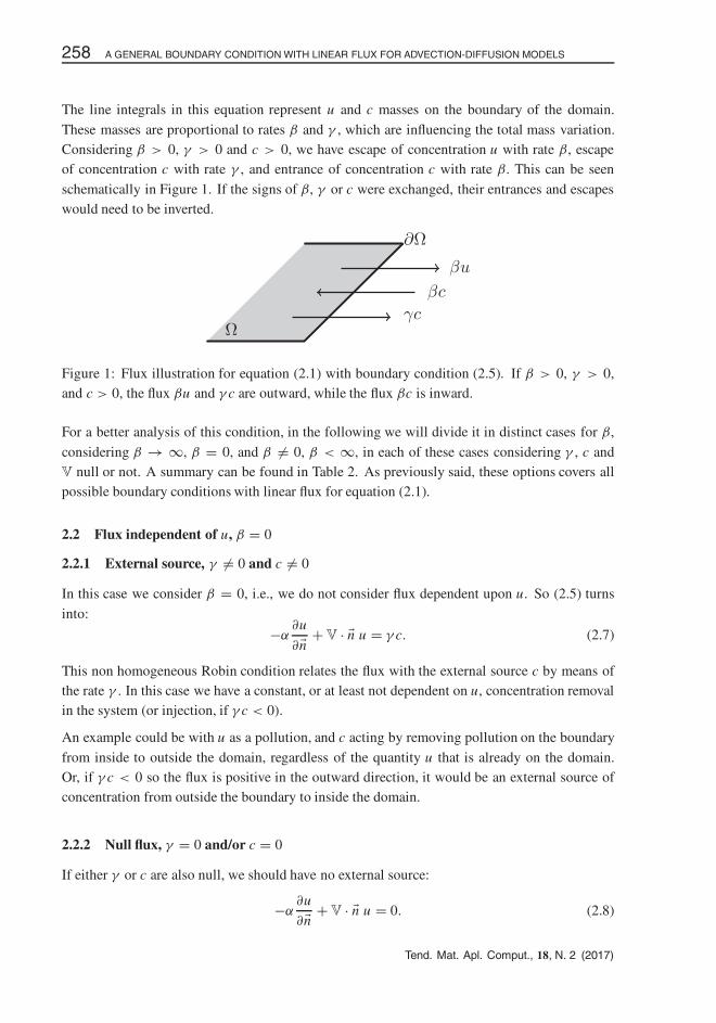
The line integrals in this equation represent u and c masses on the boundary of the domain.

These masses are proportional to rates β and γ , which are influencing the total mass variation.Considering β > 0, γ > 0 and c > 0, we have escape of concentration u with rate β, escapeof concentration c with rate γ , and entrance of concentration c with rate β. This can be seen

schematically in Figure 1. If the signs of β, γ or c were exchanged, their entrances and escapeswould need to be inverted.

βu

βc

γc

∂Ω

Ω

Figure 1: Flux illustration for equation (2.1) with boundary condition (2.5). If β > 0, γ > 0,and c > 0, the flux βu and γ c are outward, while the flux βc is inward.

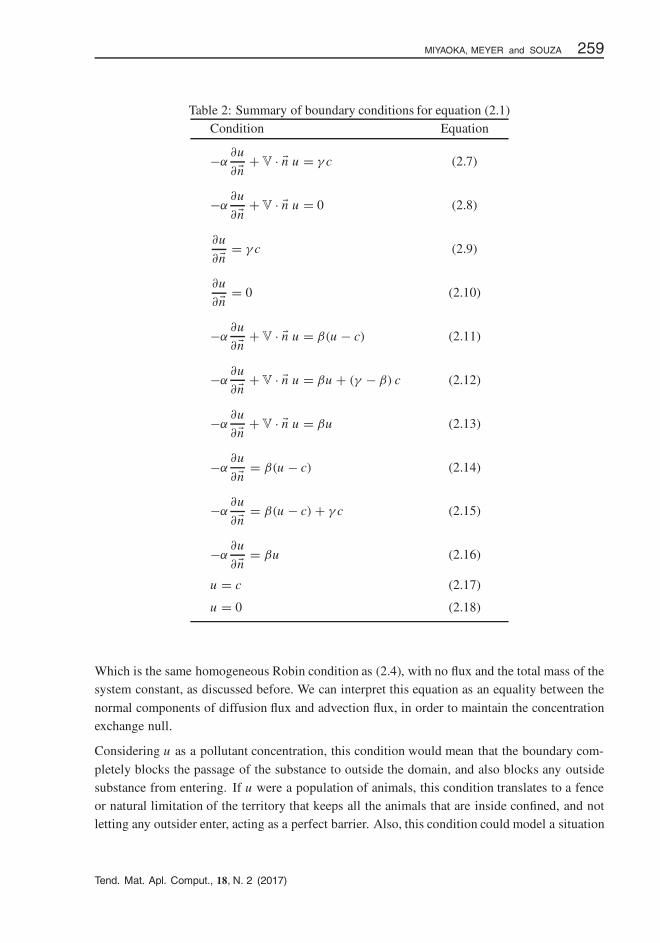
For a better analysis of this condition, in the following we will divide it in distinct cases for β,

considering β → ∞, β = 0, and β �= 0, β < ∞, in each of these cases considering γ , c andV null or not. A summary can be found in Table 2. As previously said, these options covers allpossible boundary conditions with linear flux for equation (2.1).

2.2 Flux independent of u, β = 0

2.2.1 External source, γ �= 0 and c �= 0

In this case we consider β = 0, i.e., we do not consider flux dependent upon u. So (2.5) turns

into:

−α∂u

∂ �n + V · �n u = γ c. (2.7)

This non homogeneous Robin condition relates the flux with the external source c by means ofthe rate γ . In this case we have a constant, or at least not dependent on u, concentration removalin the system (or injection, if γ c < 0).

An example could be with u as a pollution, and c acting by removing pollution on the boundary

from inside to outside the domain, regardless of the quantity u that is already on the domain.Or, if γ c < 0 so the flux is positive in the outward direction, it would be an external source ofconcentration from outside the boundary to inside the domain.

2.2.2 Null flux, γ = 0 and/or c = 0

If either γ or c are also null, we should have no external source:

−α∂u

∂ �n + V · �n u = 0. (2.8)


�

�

“main” — 2017/8/14 — 12:57 — page 259 — #7�

�

�

�

�

�


Table 2: Summary of boundary conditions for equation (2.1)Condition Equation

−α∂u

∂ �n + V · �n u = γ c (2.7)

−α∂u

∂ �n + V · �n u = 0 (2.8)

∂u

∂ �n = γ c (2.9)

∂u

∂ �n = 0 (2.10)

−α∂u

∂ �n + V · �n u = β(u − c) (2.11)

−α∂u

∂ �n + V · �n u = βu + (γ − β) c (2.12)

−α∂u

∂ �n + V · �n u = βu (2.13)

−α∂u

∂ �n = β(u − c) (2.14)

−α∂u

∂ �n = β(u − c) + γ c (2.15)

−α∂u

∂ �n = βu (2.16)

u = c (2.17)

u = 0 (2.18)

Which is the same homogeneous Robin condition as (2.4), with no flux and the total mass of thesystem constant, as discussed before. We can interpret this equation as an equality between the

normal components of diffusion flux and advection flux, in order to maintain the concentrationexchange null.

Considering u as a pollutant concentration, this condition would mean that the boundary com-

pletely blocks the passage of the substance to outside the domain, and also blocks any outsidesubstance from entering. If u were a population of animals, this condition translates to a fenceor natural limitation of the territory that keeps all the animals that are inside confined, and notletting any outsider enter, acting as a perfect barrier. Also, this condition could model a situation


�

�

“main” — 2017/8/14 — 12:57 — page 260 — #8�

�

�

�

�

�


in which the value of u is constant along the boundary, that is: everything that enters is equivalent

to whatever leaves the domain, so that the flux is null.

2.2.3 External source with no advection, γ �= 0, c �= 0 and V = 0

In the particular case of the purely diffusive problem, V = 0, and condition (2.7) simplifies to a

non homogeneous Neumann one:

−α∂u

∂ �n = γ c. (2.9)

In the purely diffusive problem the flux is given solely by the directional derivative (Fick’s law[2]), so the interpretation is the same as of (2.7).

The pollutant case is also valid as an example here, not considering the transport by makingV = 0. But another example can be the previously mentioned heat problem, with u measuring

the temperature in a metal plate and at the boundaries a fixed temperature being kept by someexternal source. Considering u as the ambient temperature, the domain could be a room isolatedfrom outer temperature, with a heater inside, represented by c.

2.2.4 Null flux with no advection, γ = 0 or c = 0 and V = 0

If γ = 0 or c = 0 in the purely diffusive case, we have the following homogeneous Neumanncondition, which is a particular case of (2.8):

∂u

∂ �n = 0. (2.10)

Continuing with the temperature example, this condition means that the boundaries are perfectly

isolated so that there is no influence of the external media to the inside temperature. This mayoccur in a metal plate or in the ambient temperature examples, without external influence.

We observe that this condition is a no flux one only for the purely diffusive case, and if appliedto the general problem (2.1), it will neglect the advective flux V · �n u. This would mean that

βu = V · �n u, with β �= 0, considering a flux due to βu that actually does not exist. Thiscondition may be interesting if the boundary in study is a barrier to diffusion, so the diffusiveflux will be null, but not a barrier to advection, leaving its flux unaltered.

2.3 Partial flux, β �= 0

2.3.1 Exchange between inside and outside, γ = 0 and c �= 0

Before proceeding to the general case, in which all the parameters in (2.5) are different from

zero, we will consider the case in which only γ = 0, i.e., only the rate due to external source istaken as zero. Then we have the following non homogeneous Robin condition:

−α∂u

∂ �n +V · �n u = β(u − c). (2.11)


�

�

“main” — 2017/8/14 — 12:57 — page 261 — #9�

�

�

�

�

�


This condition tells us that parameter β relates the flux exchange, exit or entrance, of both u and

c on the boundary. That is, if u > c, with β > 0, then concentration u along the boundary isgreater than the external source c, therefore the flux is positive to the outside and this differenceis balanced. If u < c, with β > 0, then the external source is greater than the concentration

on the boundary, and then the flux is negative as well as the sign of β (u − c), leading to aninward flux.

In the pollutant example, this condition models an exchange of concentration on the boundary,depending on both external concentration, c, and internal, u, as explained in the previous para-

graph, as an osmosis phenomenon, greater concentrations tend to migrate to locations with lowerconcentrations. Considering u as confined animals, this condition would mean that they can leaveand enter along the boundary, not freely, but accordingly to the concentration present there. So

the animals would leave the domain if the concentration were grater than c, or enter if it weresmaller than c.

2.3.2 Dependence on u and external source, γ �= 0 and c �= 0

This is the most important condition, because it includes all others. It is a non homogeneousRobin condition and arises when all the parameters in (2.5) are non zero. We rewrite it here in

two different ways for convenience:

−α∂u

∂ �n + V · �n u = βu + (γ − β) c. (2.12a)

−α∂u

∂ �n + V · �n u = β (u − c) + γ c. (2.12b)

Looking at (2.12a) we can divide the flux in two parts: one depending on u and the other on c.The greater the concentration of u on the boundary, the greater will be the exit (or entrance) of

it, being β the rate that regulates this change. If β > 0, we have entrance, and if β < 0, we haveexit of u from the domain. Also, the flux relative to (γ − β)c does not vary with u, but it candepend on x, y, t if γ , β and/or c do so. The sign of γ − β tells us if there is input into (γ > β),

or output from the domain (γ < β) of external source c.

On the other hand, looking at (2.12b), we can see that the term γ c is a constant injection ofconcentration as in (2.7), which is related to factors external to the domain. Also, the term β(u −c) is the same as in (2.11), having here the same role. So we see that β is a parameter that relates

the inside of the domain to the outside, while γ does not depend on the inside, considering onlythe contribution of external factors.

Considering again u as a concentration pollutant, this condition considers the exchange depen-dent on the external concentration, as in (2.11), but also with a constant removal as in (2.7) (or

constant source if γ c < 0).


�

�

“main” — 2017/8/14 — 12:57 — page 262 — #10�

�

�

�

�

�


2.3.3 Dependence on u, γ = 0 and c = 0

In the case γ = β, or c = 0, (2.11) becomes a homogeneous Robin condition:

−α∂u

∂ �n + V · �n u = βu. (2.13)

This condition relates the flux only with the density along the boundary, without external factors.If β > 0, this condition means that the flux is outward positive so, as u increases, the exit ofconcentration from the domain becomes higher. If β < 0, we have the opposite. We note that

this is a particular case of (2.11) without an external balance factor, so that the behavior of theflux does not depend on the outside of the domain.

An example could be either the pollutant or the animals case, in a boundary which allows passage,similar to that of (2.11) but without contributions from the outside. According to [28], this is the

standard boundary condition for equation (2.1).

2.3.4 Dependence on u, γ = β, c �= 0

In this case, the condition also reduces to (2.13), but there is a conceptual difference: the externalsource c is not null, but the equality between the rates γ and β causes the whole term (γ − β)cin (2.12a) to vanish, so that there is an equality between the entrance and exit of c in the domain:

βc = γ c (which is entrance or exit depends on the signs involved).

This situation is highly unlikely because the model is an approximation of the reality, thereforeparameters considered do not have precise values. A possible example could be, in the pollutantcase, an artificial regulation of γ , in order to precisely cause the equality γ = β, if one can

control the entrance/exit of the pollutant.

2.3.5 Exchange between inside and outside with no advection, γ = 0, c �= 0 and V = 0

Considering now the purely diffusive case, V = 0, and γ = 0, we have:

−α∂u

∂ �n = β(u − c), (2.14)

with same interpretation as in (2.11). The example in (2.11) about the pollutant is also valid here,but a typical example is the temperature case, this condition being known as the heat radiation

boundary [3], where there is heat exchange with the external media. In this fashion, c representsthe external temperature, and the boundary condition balances the difference in the temperaturefrom inside the domain and outside, with the same analysis as in (2.11).

2.3.6 Dependence on u and external source with no advection, γ �= 0, c �= 0 and V = 0

In the purely diffusive case, V = 0, the general linear condition is:

−α∂u

∂ �n = β(u − c) + γ c, (2.15)


�

�

“main” — 2017/8/14 — 12:57 — page 263 — #11�

�

�

�

�

�


which is a particular case of (2.12), just without the advection term, so the same interpretation

is valid. Again considering u as the ambient temperature in a room, this combines the radiationboundary in (2.14) and the external source in (2.9), so that there is an exchange of temperaturewith the exterior of the room and an internal source of heat.

2.3.7 Dependence on u with no advection, γ = 0 or c = 0 and V = 0

If, besides V = 0, either γ = 0 or c = 0, we have an homogeneous Robin condition:

−α∂u

∂ �n = βu, (2.16)

which is a particular case of (2.13).

In the heat diffusing in a metal plate, this means that there is change of temperature in the ex-

tremes of the plate, which does not depend on the outside, but only on the temperature along theboundary.

2.4 Total flux, β → ∞2.4.1 Total flux with external source, c �= 0

Rewriting condition (2.5) in order to isolate u − c, we obtain:

1

β

(−α

∂u

∂ �n + V · �n u − γ c

)= u − c.

Increasing the flow due to the presence of u in the boundary indefinitely, i.e. considering unlim-ited growth of β, so that β → ∞, we have the following non homogeneous Dirichlet condition:

u = c. (2.17)

This tells us that all concentration u that arrives on the boundary dissipates, because the flux dueto β is unlimited, thereby the value of u is completely described by the external source c.

In the pollution example, the unlimited growth of β means that all the pollution arriving on the

boundary crosses it completely, or is totally absorbed, so that the only concentration of pollutantthat remains there is due to the external source c.

2.4.2 Total flux without external source, c = 0

If besides β → ∞ we also have c = 0, we obtain the homogeneous Dirichlet condition, whichalso has total exit flux but without external source, keeping the concentration zero along the

boundary:u = 0. (2.18)


�

�

“main” — 2017/8/14 — 12:57 — page 264 — #12�

�

�

�

�

�


In the pollution case, we also have a complete passage of concentration, but without any source,

so that the concentration remains zero on the boundary. In a population dispersal case, this con-dition can be used in a situation in which no animal can stay along the boundary, because of theterrain, for example.

We note that the same conditions, (2.17) or (2.18) are valid if α = 0, V = 0, or even γ = 0,

thereby the total flux condition is independent of these quantities.

2.5 Mixed boundary conditions

In practical situations, mathematical models often consider domains with heterogeneous bound-

aries. This means that the boundary ∂� must be separated in several regions ∂�i , i = 1, . . . , N ,with ∂� = ∪N

i=1∂�i , the union being disjoint. Each of these regions ∂�i can then be modeledby any of the presented boundary conditions (2.7)–(2.18). Most of the already mentioned worksutilize this kind of mixed boundary conditions in their models. In particular, in [10] the authors

explain each part of the boundary considered for an air/lake pollution model.

3 NUMERICAL SIMULATIONS

In order to obtain numerical approximations to solutions of problem (2.1), we utilized second

order Finite Difference formulas in spatial variables and Crank–Nicolson Method in the timevariable [30]. For simplicity we considered a rectangular domain � = [0, L] × [0, H ]. Forboundary points we applied the finite difference formulas directly in the boundary conditions

obtaining complementary equations. We then obtained an algebraic linear system to be solved ateach time step, which is solved by the LU factorization method. As the system matrix is constant,it may be factorized only once. Matlab was used for the implementation of the computationalroutines. Details about the numerical solutions calculations can be found in the Appendix.

The illustrative parameters utilized were α = 0.1; V = (0.02, 0.02); β = 0, β = 0.1, β = 0.05,or β = 100; γ = 0, γ = 0.1 or γ = 0.05; c = 0, c = 1 or c = −1. The length andheight of the domain were L = H = 1, and the time interval J = (0, 2]. The domain wasdiscretized using 26 intervals in both x and y direction and 210 in time. The initial condition was

u0(x, y) = κ exp(−64((x − 0.5)2 + (y − 0.5)2)), a gaussian at the center of the domain, whereκ is a constant to maintain initial mass equal to the unit. This gaussian was chosen because it hasnegligible value on the boundary of the domain. Therefore at the beginning of the simulations,

the boundary is unaffected. As one can obtain any of the exposed boundary conditions from (2.5),this general expression was used in the implementation, and the parameters adjusted to obtainthe different conditions.

Our computational experiments aim to illustrate some of the cases exposed in the previous sec-

tion, focusing on the total mass of the system as a function of time, M(t). This mass is calcu-lated by numerical integration, with repeated Simpson’s formula, using the numerical solutionobtained. More precisely, we obtain numerical approximations to the solutions of problem (2.1),

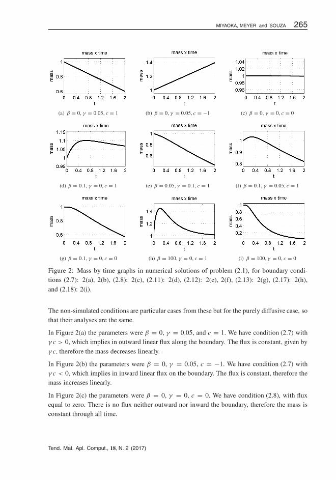
with boundary conditions (2.7), (2.8), (2.11), (2.12), (2.13), (2.17), and (2.18), Figure 2.


�

�

“main” — 2017/8/14 — 12:57 — page 265 — #13�

�

�

�

�

�


(a) β = 0, γ = 0.05, c = 1 (b) β = 0, γ = 0.05, c = −1 (c) β = 0, γ = 0, c = 0

(d) β = 0.1, γ = 0, c = 1 (e) β = 0.05, γ = 0.1, c = 1 (f) β = 0.1, γ = 0.05, c = 1

(g) β = 0.1, γ = 0, c = 0 (h) β = 100, γ = 0, c = 1 (i) β = 100, γ = 0, c = 0

Figure 2: Mass by time graphs in numerical solutions of problem (2.1), for boundary condi-tions (2.7): 2(a), 2(b), (2.8): 2(c), (2.11): 2(d), (2.12): 2(e), 2(f), (2.13): 2(g), (2.17): 2(h),

and (2.18): 2(i).

The non-simulated conditions are particular cases from these but for the purely diffusive case, sothat their analyses are the same.

In Figure 2(a) the parameters were β = 0, γ = 0.05, and c = 1. We have condition (2.7) withγ c > 0, which implies in outward linear flux along the boundary. The flux is constant, given by

γ c, therefore the mass decreases linearly.

In Figure 2(b) the parameters were β = 0, γ = 0.05, c = −1. We have condition (2.7) withγ c < 0, which implies in inward linear flux on the boundary. The flux is constant, therefore themass increases linearly.

In Figure 2(c) the parameters were β = 0, γ = 0, c = 0. We have condition (2.8), with fluxequal to zero. There is no flux neither outward nor inward the boundary, therefore the mass isconstant through all time.


�

�

“main” — 2017/8/14 — 12:57 — page 266 — #14�

�

�

�

�

�


In Figure 2(d) the parameters were β = 0.1, γ = 0, c = 1. We have condition (2.11), with

exchange between internal and external concentration, given by u and c respectively. At thebeginning there is inward flux, because u < c on the boundary, therefore the mass increases.But after (approximately at t = 0.6), the flux becomes outward, as the concentration along the

boundary increases making u > c, and the mass decreases.

In Figure 2(e) the parameters were β = 0.05, γ = 0.1, c = 1. We have condition (2.12), withthe combined effects of (a) and (d). Therefore the flux is always outward because of the term γ c,but it starts small and increases because of β(u − c). The mass always decreases.

In Figure 2(f) the parameters were β = 0.1, γ = 0.05, c = 1. We have condition (2.12), but

with β < γ , therefore the flux due to c in inward, causing the concentration to increase at thebeginning. As the system mass increases, so does the term βu, and the flux becomes outward(approximately at t = 0.3), causing the mass to decrease.

In Figure 2(g) the parameters were β = 0.1, γ = 0, c = 0. We have condition (2.13), with flux

dependent only on u. As in the very beginning there is no concentration on the boundary, themass remains constant. But as concentration increases along the boundary, so does the outwardflux, causing the mass to decrease.

In Figure 2(h) the parameters were β = 100, γ = 0, c = 1. We have condition (2.17), with total

flux is outward the domain, and also a total injection due to c. At the beginning there is an increasein the mass, because there is only injection. Afterwards there is a decrease in concentration dueto the total outward flux.

In Figure 2(i) the parameters were β = 100, γ = 0, c = 0. We have condition (2.18), with total

flux outward and no external source. The flux becomes higher as the concentration starts to crossthe boundary causing the mass to decrease.

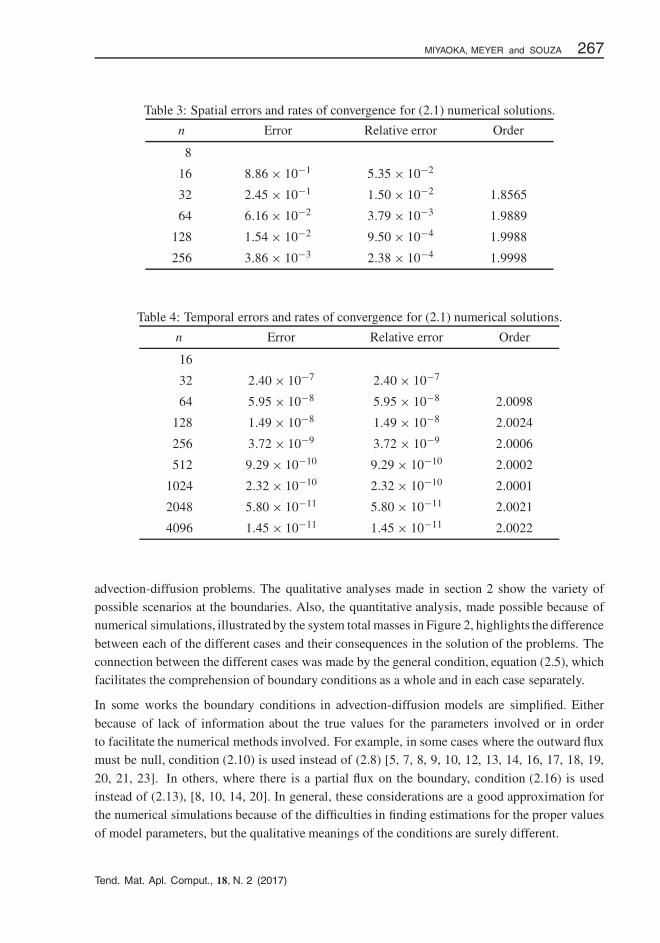
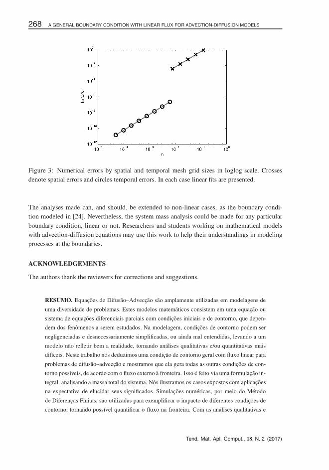
In Tables 3 and 4 we show convergence tests for our numerical solutions. In each table we showabsolute and relative errors in max norm obtained comparing solutions in consecutive meshes,

which consist in regular subdivisions of the domain. In Table 3, n denotes the number of divisionsin x and y directions, which are equal, and in Table 4, n is the number of divisions in time t . Forthe temporal convergence, we used the mass of the system M(t) for the errors, which contains

information of the whole spatial domain. We also show the numerical rate of convergence ofthe methods comparing two consecutive errors. As expected, both in space and time the ratesobtained converge to 2, since the methods used have �x2, �y2 and �t2 orders. In Figure 3 we

show an error by mesh grid sizes loglog graph for both spatial and temporal analyses, with linearfits for each case. These results collaborate to the accuracy of the results obtained.

4 CONCLUSION

In this work, we show that one unique general boundary condition with linear flux, equation (2.5),

generates all other particular cases. We also show, by means of qualitative analysis and numericalsimulations, the interpretations and importance of boundary conditions in different situations in


�

�

“main” — 2017/8/14 — 12:57 — page 267 — #15�

�

�

�

�

�


Table 3: Spatial errors and rates of convergence for (2.1) numerical solutions.

n Error Relative error Order

8

16 8.86 × 10−1 5.35 × 10−2

32 2.45 × 10−1 1.50 × 10−2 1.8565

64 6.16 × 10−2 3.79 × 10−3 1.9889

128 1.54 × 10−2 9.50 × 10−4 1.9988

256 3.86 × 10−3 2.38 × 10−4 1.9998

Table 4: Temporal errors and rates of convergence for (2.1) numerical solutions.

n Error Relative error Order

16

32 2.40 × 10−7 2.40 × 10−7

64 5.95 × 10−8 5.95 × 10−8 2.0098

128 1.49 × 10−8 1.49 × 10−8 2.0024

256 3.72 × 10−9 3.72 × 10−9 2.0006

512 9.29 × 10−10 9.29 × 10−10 2.0002

1024 2.32 × 10−10 2.32 × 10−10 2.0001

2048 5.80 × 10−11 5.80 × 10−11 2.0021

4096 1.45 × 10−11 1.45 × 10−11 2.0022

advection-diffusion problems. The qualitative analyses made in section 2 show the variety ofpossible scenarios at the boundaries. Also, the quantitative analysis, made possible because ofnumerical simulations, illustrated by the system total masses in Figure 2, highlights the difference

between each of the different cases and their consequences in the solution of the problems. Theconnection between the different cases was made by the general condition, equation (2.5), whichfacilitates the comprehension of boundary conditions as a whole and in each case separately.

In some works the boundary conditions in advection-diffusion models are simplified. Either

because of lack of information about the true values for the parameters involved or in orderto facilitate the numerical methods involved. For example, in some cases where the outward fluxmust be null, condition (2.10) is used instead of (2.8) [5, 7, 8, 9, 10, 12, 13, 14, 16, 17, 18, 19,

20, 21, 23]. In others, where there is a partial flux on the boundary, condition (2.16) is usedinstead of (2.13), [8, 10, 14, 20]. In general, these considerations are a good approximation forthe numerical simulations because of the difficulties in finding estimations for the proper values

of model parameters, but the qualitative meanings of the conditions are surely different.


�

�

“main” — 2017/8/14 — 12:57 — page 268 — #16�

�

�

�

�

�


Figure 3: Numerical errors by spatial and temporal mesh grid sizes in loglog scale. Crossesdenote spatial errors and circles temporal errors. In each case linear fits are presented.

The analyses made can, and should, be extended to non-linear cases, as the boundary condi-tion modeled in [24]. Nevertheless, the system mass analysis could be made for any particular

boundary condition, linear or not. Researchers and students working on mathematical modelswith advection-diffusion equations may use this work to help their understandings in modelingprocesses at the boundaries.

ACKNOWLEDGEMENTS

The authors thank the reviewers for corrections and suggestions.

RESUMO. Equacoes de Difusao–Adveccao sao amplamente utilizadas em modelagens de

uma diversidade de problemas. Estes modelos matematicos consistem em uma equacao ou

sistema de equacoes diferenciais parciais com condicoes iniciais e de contorno, que depen-

dem dos fenomenos a serem estudados. Na modelagem, condicoes de contorno podem ser

negligenciadas e desnecessariamente simplificadas, ou ainda mal entendidas, levando a um

modelo nao refletir bem a realidade, tornando analises qualitativas e/ou quantitativas mais

difıceis. Neste trabalho nos deduzimos uma condicao de contorno geral com fluxo linear para

problemas de difusao–adveccao e mostramos que ela gera todas as outras condicoes de con-

torno possıveis, de acordo com o fluxo externo a fronteira. Isso e feito via uma formulacao in-

tegral, analisando a massa total do sistema. Nos ilustramos os casos expostos com aplicacoes

na expectativa de elucidar seus significados. Simulacoes numericas, por meio do Metodo

de Diferencas Finitas, sao utilizadas para exemplificar o impacto de diferentes condicoes de

contorno, tornando possıvel quantificar o fluxo na fronteira. Com as analises qualitativas e


�

�

“main” — 2017/8/14 — 12:57 — page 269 — #17�

�

�

�

�

�


quantitativas, este trabalho pode ser util a pesquisadores e estudantes trabalhando em mode-

los matematicos com equacoes de difusao–adveccao.

Palavras-chave: condicoes de contorno, equacoes diferenciais parciais, modelos matemati-

cos, simulacoes computacionais.

REFERENCES

[1] J. Fourier. Theorie analytique de la chaleur, par M. Fourier. Paris: Chez Firmin Didot, pere et fils,(1822).

[2] A. Okubo & S.A. Levin. Diffusion and ecological problems: modern perspectives, vol. 14. New York:

Springer Science & Business Media, (2013).

[3] T.L. Bergman, F.P. Incropera, D.P. DeWitt & A.S. Lavine. Fundamentals of heat and mass transfer.Jefferson City: John Wiley & Sons, (2011).

[4] G.I. Marchuk. Mathematical models in environmental problems, vol. 16. North-Holland: Elsevier,(2011).

[5] D.C. Mistro. “O problema da poluicao em rios por mercurio metalico: modelagem e simulacao

numerica”. Master’s thesis, DMA, IMECC, UNICAMP, Campinas, SP, (1992).

[6] J.F.C.A. Meyer, R.F. Cantao & I.R.F. Poffo. “Oil spill movement in coastal seas: modelling andnumerical simulations”. WIT Trans. Ecol. Envir., 27 (1998), 23–32.

[7] E.C.C. Poletti & J.F.C.A. Meyer. “Numerical methods and fuzzy parameters: an environmental im-

pact assessment in aquatic systems”. Comput. Appl. Math., pp. 1–12, (2016).

[8] A. Krindges. Modelagem e simulacao computacional de um problema tridimensional de difusao-

adveccao com uso de Navier-Stokes. PhD thesis, DMA, IMECC, UNICAMP, Campinas, SP, (2011).

[9] S.E.P. Castro. “Modelagem matematica e aproximacao numerica do estudo de poluentes no ar”. Mas-

ter’s thesis, DMA, IMECC, UNICAMP, Campinas, SP, (1993).

[10] J.F.C.A. Meyer & G.L. Diniz. “Pollutant dispersion in wetland systems: Mathematical modelling and

numerical simulation.” Ecol. Model., 200(3) (2007), 360–370.

[11] D. Buske, M.T. Vilhena, T. Tirabassi & B. Bodmann. “Air pollution steady-state advection-diffusionequation: the general three-dimensional solution”. Journalof Environmental Protection, 3(09) (2012),

1124.

[12] G.L. Diniz. “A mudanca no habitat de populacoes de peixes: de rio a represa – o modelo matematico”.Master’s thesis, DMA, IMECC, UNICAMP, Campinas, SP, (1994).

[13] T.M.V.S. Lacaz. Analises de problemas populacionais intraespecıficos e interespecıficos com difusao

densidade-dependente. PhD thesis, DMA, IMECC, UNICAMP, Campinas, SP, (1999).

[14] M.T. Koga. Dinamica populacional da Mosca-dos-chifres (Haematobia Irritans) em um ambiente

com competicao: simulacoes computacionais. PhD thesis, FEEC, UNICAMP, Campinas, SP, (2015).

[15] J.R. Sibert, J. Hampton, D.A. Fournier & P.J. Bills. “An advection-diffusion-reaction model for the

estimation of fish movement parameters from tagging data, with application to skipjack tuna (katsu-wonus pelamis)”. Can. J. Fish. Aquat. Sci., 56(6) (1999), 925–938.


�

�

“main” — 2017/8/14 — 12:57 — page 270 — #18�

�

�

�

�

�


[16] M.M. Salvatierra. “Modelagem matematica e simulacao computacional da presenca de materiais im-

pactantes toxicos em casos de dinamica populacional com competicao inter e intra-especıfica,” Mas-ter’s thesis, DMA, IMECC, UNICAMP, Campinas, SP, (2005).

[17] R.C. Sossae. A presenca evolutiva de um material impactante e seu efeito no transiente populacional

de especies interativas. PhD thesis, DMA, IMECC, UNICAMP, Campinas, SP, (2003).

[18] D.C. Guaca. “Impacto ambiental em meios aquaticos: modelagem, aproximacao e simulacao de um

estudo na baıa de Buenaventura-Colombia”. Master’s thesis, DMA, IMECC, UNICAMP, Campinas,SP, (2015).

[19] L.C. Abreu. “Influencia de poluentes sobre macroalgas na Baıa de Sepetiba, RJ: modelagem

matematica, analise numerica e simulacoes computacionais”. Master’s thesis, DMA, IMECC, UNI-CAMP, Campinas, SP, (2009).

[20] L. Torre, P.C.C. Tabares, F. Momo, J.F.C.A. Meyer & R. Sahade. “Climate change effects on antarcticbenthos: a spatially explicit model approach”. Climatic Change, 141(4) (2017), 733–746.

[21] S. Pregnolatto. Mal-das-cadeiras em capivaras: estudo, modelagem e simulacao de um caso. PhD

thesis, DMA, IMECC, UNICAMP, Campinas, SP, (2002).

[22] M. Missio. Modelos de EDP integrados a logica Fuzzy e metodos probabilısticos no tratamento

de incertezas: uma aplicacao a febre aftosa em bovinos. PhD thesis, DMA, IMECC, UNICAMP,

Campinas, SP, (2008).

[23] J.M.R. Souza. “Estudo da dispersao de risco de epizootias em animais: o caso da influenza aviaria”.

Dissertacao de Mestrado, DMA, IMECC, UNICAMP, Campinas, SP, (2010).

[24] R.S. Cantrell & C. Cosner. “On the effects of nonlinear boundary conditions in diffusive logisticequations on bounded domains”. J. Differ. Equations, 231(2) (2006), 768–804.

[25] C. Cosner & Y. Lou. “Does movement toward better environments always benefit a population?”. J.

Math. Anal. Appl., 277(2) (2003), 489–503.

[26] V. Mendez, D. Campos, I. Pagonabarraga, & S. Fedotov. “Density-dependentdispersal and populationaggregation patterns,” J. Theor. Biol., 309 (2012), 113–120.

[27] N. Shigesada, K. Kawasaki & H.F. Weinberger. “Spreading speeds of invasive species in a periodicpatchy environment: effects of dispersal based on local information and gradient-based taxis”. Jpn. J.

Ind. Appl. Math., 32(3) (2015), 675–705.

[28] R.S. Cantrell & C. Cosner. Spatial ecology via reaction-diffusion equations. Chichester: John Wiley& Sons, (2004).

[29] B.P. Boudreau. Diagenetic Models and Their Implementation, vol. 505. Berlin: Springer Berlin,

(1997).

[30] R.J. LeVeque. Finite difference methods for ordinary and partial differential equations: steady-state

and time-dependent problems, vol. 98. Philadelphia: Siam, (2007).

APPENDIX

In this appendix we describe the calculation of numerical solutions for problem (2.1) with thegeneral boundary condition (2.5), using second order Finite Difference formulas in spatial vari-ables and Crank-Nicolson Method in the time variable [30]. Considering a square domain


�

�

“main” — 2017/8/14 — 12:57 — page 271 — #19�

�

�

�

�

�


� = [0, L]×[0, H ], with partitions {x1, . . . , xn+1}×{y1, . . . , yn+1} for � and {t1, . . . , tm+1} for

I = [t0, t f ], we use the notation u(xi , y j , tk) = uki, j for i, j =, 1 . . . , n+1, and k = 1, . . . , m+1.

The difference formulas used were:

∂uki, j

∂x≈ uk

i+1, j − uki−1, j

2�x,

∂2uki, j

∂x2≈ uk

i+1, j − 2uki, j + uk

i−1, j

�x2,∂u

n+ 12

i, j

∂t≈ uk+1

i, j − uki, j

�t

∂uki, j

∂y≈ uk

i, j+1 − uki, j−1

2�y,

∂2uki, j

∂y2≈ uk

i, j+1 − 2uki, j + uk

i, j−1

�y2, u

n+ 12

i, j ≈ uk+1i, j + uk

i, j

2

Applying these formulas in (2.1) we obtain:(

− α�t

2�x2 − v�t

4�x

)uk+1

i−1, j +(

− α�t

2�y2 + w�t

4�y

)uk+1

i, j−1

+(

1 + α�t

�x2+ α�t

�x2

)uk+1

i, j +(

− α�t

2�y2+ w�t

4�y

)uk+1

i, j+1

+(

− α�t

2�x2+ v�t

4�x

)uk+1

i+1, j =(

α�t

2�x2+ v�t

4�x

)uk

i−1, j

+(

α�t

2�y2+ w�t

4�y

)uk

i, j−1 +(

1 − α�t

�x2− α�t

�x2

)uk

i, j

+(

α�t

2�y2− w�t

4�y

)uk

i, j+1 +(

α�t

2�x2− v�t

4�x

)uk

i+1, j

(4.1)

For points at the boundary, we need to apply the difference formulas on boundary condition (2.5).

We then obtain, for any k, where �n = (n1, n2):

− αn1�t

2�xuk

i+1, j + αn1�t

2�xuk

i−1, j − αn2�t

2�yuk

i, j+1

+ αn2�t

2�yuk

i, j−1 + (vn1 + wn2 − β) uki, j = (γ − β)c.

For each side of the rectangular domain, we have different normal vectors �n, which lead us to thefollowing expressions, plugged in (4.1) for inexistent points of the mesh grid, for any k:

�n = (−1, 0) ⇒ uki−1, j = uk

i+1, j − 2�x

α

[(v + β)uk

i, j + (γ − β)c]

.

�n = (0, −1) ⇒ uki, j−1 = uk

i, j+1 − 2�y

α

[(w + β)uk

i, j + (γ − β)c].

�n = (1, 0) ⇒ uki+1, j = uk

i−1, j + 2�x

α

[(v − β)uk

i, j − (γ − β)c].

�n = (0, 1) ⇒ uki, j+1 = uk

i, j−1 + 2�y

α

[(w − β)uk

i, j − (γ − β)c]

.

(4.2)


�

�

“main” — 2017/8/14 — 12:57 — page 272 — #20�

�

�

�

�

�


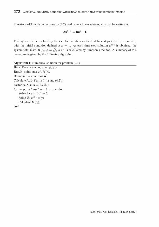
Equations (4.1) with corrections by (4.2) lead us to a linear system, with can be written as:

Auk+1 = Buk + f.

This system is then solved by the LU factorization method, at time steps k = 1, . . . , m + 1,with the initial condition defined at k = 1. As each time step solution uk+1 is obtained, thesystem total mass M(tk+1) = ∫∫

�u d A is calculated by Simpson’s method. A summary of this

procedure is given by the following algorithm.

Algorithm 1: Numerical solution for problem (2.1).Data: Parameters: α, v, w, β, γ , c.Result: solutions: uk , M(t).

Define initial condition u0;Calculate A, B, f as in (4.1) and (4.2);Factorize A as A = LAUA;

for temporal iteration = 1, . . . , nt doSolve LAy = Buk + f;Solve UAuk+1 = y;

Calculate M(tk);end


Documents

18, N. 2 (2017), 253-272 Tema