18 placing safety - SciELO · The aim of this paper is to solve the problem of placing safety stock over a Logistic Network (LN) that is represented by a Generic Bill of Materials

Vol.�12,�June�2014�538�

�

Placing Safety Stock in Logistic Networks under Guaranteed-Service Time Inventory Models: An Application to the Automotive Industry L. A. Moncayo-Martínez*1,2, E. O. Reséndiz-Flores2, D. Mercado2 and C. Sánchez-Ramírez3

1 Department of Industrial and Operation Engineering Instituto Tecnológico Autónomo de México (ITAM) México, D. F., México *[email protected] 2 Division of Postgraduate Studies and Research The Technological Institute of Saltillo Saltillo, Coahuila, México 3 División de Ciencias e Ingeniería Department of Industrial Engineering & Manufacturing Science Orizaba Institute of Technology Orizaba, Veracruz, México ABSTRACT The aim of this paper is to solve the problem of placing safety stock over a Logistic Network (LN) that is represented by a Generic Bill of Materials (GBOM). Thus the LN encompasses supplying, assembling, and delivering stages. We describe, in detail, the recursive algorithm based on Dynamic Programming (DP) to solve the placing safety stock problem under guaranteed-service time models. We also develop a java-based application (JbA) that both models the LN and runs the recursive DP algorithm. We solved a real case of a company that manufactures fixed brake and clutch pedal modules of cars’ brake system. After running JbA, the levels of inventory decreased by zero in 55 out of 65 stages. Keywords: Safety Stock, Guaranteed-service time, Dynamic Programming, Automotive Industry. RESUMEN El objetivo de este artículo es resolver el problema de colocación inventario en una Red Logística (LN) que es representada por una Lista de Materiales Genérica (GBOM), de manera que la LN tiene etapas de suministro, ensamble y entrega. Describimos, a detalle, el algoritmo recursivo de Programación Dinámica (DP) para resolver el problema de colocación de inventario en modelos de servicio garantizado. También programamos una aplicación en java (JbA) que modela la LN y ejecuta las operaciones recursivas del algoritmo de DP. Resolvimos un caso real de una empresa que manufactura módulos de frenos y pedales del clutch del sistema de frenos utilizados en los autos. Los resultados muestran que los niveles de inventarios se reducen a cero en 55 de 65 etapas después de ejecutar nuestra JbA. ��1. Introduction Manufacturing companies are highly pressured into producing quality products and delivering them to the right location, at the right quantity or amount, and at the right place, subject to reduce both manufacturing and logistic costs. In order to reach this aim, companies have realised that a global approach is required to coordinate operations across the entire Logistic Network (LN) or Supply Chain, e.g. share information to minimise the bullwhip effect [1]; pass products' demand to upstream members to reduce inventory levels [2]

or solve the routing and inventory problem simultaneously [23,26]. Moreover, companies have to dynamically evaluate the LN operations [24] and reduce the complexity generated by the product diversification [25] to reach the global aim of cost reduction.

Global inventory management is an important strategy in reducing manufacturing and logistic costs because a proper inventory policy could result in reducing the amount of safety and pipeline stock.

Placing�Safety�Stock�in�Logistic�Networks�under�GuaranteedͲService�Time�Inventory�Models:�An�Application�to�the�Automotive�Industry,�L.�A.�MoncayoͲMartínez et�al.�/�538Ͳ550�

Journal�of�Applied�Research�and�Technology 539

In literature, the problem of placing inventory is divided into single stage and multi stages. The first one is a difficult but well studied problem, the models used to solve it are deterministic (e.g. economic order quantity and wagner-whitin model) and stochastic (e.g. (r,Q) and (s,S) policies)[3]. The multi stage problem could be either stochastic-service (SS) or guaranteed-service (GS). The main difference between SS and GS is the way in which a stage supplies components or assemblies to other downstream stages. Backorders are allowed in SS multi stage problem, i.e. a fraction of an order cannot be filled at the right time due to a lack of available supply [4-5]. Unlike SS model, the GS model must serve the complete order just in a guaranteed-service time Z. Our paper deals with GS models in multi stages, thus the problem is to minimise the cost of the safety stock that every stage must hold in order to serve its downstream stages just in the Z� given that the days of inventory required are U = G�+ t - Z, where G is the time in which a stage must be served by its upstream stages and t is the time spent by a stage to perform its task. The novelties of the proposed paper lie in the methodology employed to solve a real-life LN and in the java-based application programmed to solve the DP algorithm used to solve the GS inventory placing problem [2]. Additionally, we provide a pseudo code full of practical insights to carry out the recursive operations. We implemented and applied the GS time inventory model (GSTIM) to a company that manufactures fixed brake and clutch pedal modules. We both selected the product with the highest demand and described the steps followed to collect the necessary information to run the java-based application. In the following section, a literature review of the GSTIM is provided. In section 3, the model is defined and some assumptions are stated. In section 4, the methodology used to implement the GS model is depicted, so also the DP algorithm and the java-based application are described. A real case is described in section 5. Finally, results are presented in section 6 and we draw some conclusions in section 7.

2. Related Literature In this section, we cite a set of approaches related to GSTIM. Back in 1958, Simpson [6] solved the problem of placing inventory over a serial process. Adjacent stages were coupled together to equate the incoming service time of a downstream stage with the outbound service time of its upstream stage. The optimum inventory level per stage was found by determining the service time. It was proven that the optimal service time in serial processes is found in an extreme point property where the outgoing service time is equal to either zero or its incoming service time plus its processing time, i.e. using an all-or-nothing inventory policy. A boundary demand is used, thus it is interpreted as the amount of inventory a company wants to satisfy from its safety stock. Later, the same problem was solved by standard operations of DP in [7] and was extended to supply chains modelled as assembly networks [8], to distribution networks [9], and to spanning trees [10]. In a recent approach, a stage could include more than one upstream or downstream stage [2,11], so we have to notice two important facts: i) in case a downstream stage is served by multiple upstream stages, the downstream stage has to wait for the component with the longest service time, and ii) in case an upstream stage serves multiple downstream stages, the upstream stage quotes the same service time to all the adjacent downstream stages. Moreover, the assumption about demand boundary remains and it is supposed that the LN is designed already, thus the time and cost of every stage is known. The complexity of the aforementioned approach has been proven to be NP-hard [12, 13]. As a result, modification to the DP algorithms have appeared in literature to solve bigger instances than those solved efficiently using the DP standard algorithm, e.g. CPLEX is used to iteratively solve a piecewise-linear demand once redundant constrains are added [14]; branch and bound algorithm is used to reduce complexity [15]; tailor-made heuristic has been proposed [16]; and general purpose genetic algorithms are used to solve the problem [17]. Other generalizations that do not apply to our real-life case included: capacity constraints [18], LN design constraints [19], non-stationary demand [20], and stochastic lead times [21].


Vol.�12,�June�2014�540�

3. Problem Definition The problem is represented by a network G={V,E}, in which the set of vertices represents the different stages s, V={1,…,s,…,S} where S is the total number of stages. The set of edges represents the relationship among the stages, E={(1,s),…,(s,s'),…,(s',S)} where (s,s') means that s' is a downstream stage of s or s is an upstream of s'. As stated in section 1, there are: a subset of supplying stages (P�V) that provide the components or raw material; a subset of assembling stages that manufacture a sub- or final assembly (A�V); and a subset of delivering stages (D�V) which each one represents a customer who asked for a specific product. Notice that if a customer asks for m products, then there are m delivering stages. Therefore, if n customers ask for mn products, the LN has nn

m¦ delivering

stages (s�D). In order to mathematically define the problem, we describe four important assumptions. First, the demand at every stage s for W periods of time is bounded to Fs(W) and the demand at stage s is a random uncorrelated variable x(W) with mean

� �sx W and standard deviation Vs(W). Fs(W� is set by companies as a service policy, thus if we assume

that x(W)~N(P,V), then Fs(W) = � �sx W + Ks�Vs(W) where Ks is a given safety factor. Second, every stage has a periodic-review base-stock replenishment inventory policy with common review period, thus all stages s�V place their demand (multiple by a scalar I(s',s)) on their upstream stages s' at the common review period. Moreover, the base stock policy (Bs) is set to Bs = Fs(W), so the average amount of safety stock at

stage s is Is =Fs(W) - � �sx W = Ks�Vs(W) . As the demand is a random uncorrelated variable, then �Vs(W) =Vs W (see [6]), where Vs is the standard deviation over a unit of time. Third, each stage quotes a guaranteed-service time (Zs) to their downstream stages, hence s will fulfil every demand occurred at time U = Gs�+ ts - Zs, (notice that W�= U) where Gs = ':( ', )max s s s E� {Zs’} , i.e. the

net replenishment time is equal to the replenishment time (Gs�+ ts ) minus the guaranteed service time. In practise, U stands for the days of inventory required to serve a downstream stage in Z days. According to the assumptions, the problem to find the guaranteed-service times per stage that minimised the safety stock is [2]:

s s s s s sMin h C k tV G Z� �¦ (1)

Gs + ts – Zs � 0 (2) Gs’ - Zs � 0, � s:(s,s’)� E (3) Zs � :�� s� D (4) Gs, Zs � 0 and integers � s� V (5) where h is the per-unit holding cost and Cs is the cumulative cost at stage s computed by

'':( ', )s s ss s sC c C �¦ where cs is the cost at stage

s. Eq. 1 is the objective function that minimises the total safety stock. Eq. 2 assures that the days of inventory are non-negative, thus the service times are feasible. Eq. 3 guarantees that for a stage s:(s,s’)� E the guaranteed-service time Zs is not greater than the time in which the stage s' must be served. Eq. 4 assures the guaranteed-service time to the delivering stages (s� D) must be no greater than the user-defined maximum (:). Finally, the times must be non-negative and integer (Eq. 5). 4. Problem Solution The proposed framework encompasses seven steps depicted in Figure 1. The first step of the framework is to build the GBOM, in which the goes-into relationships can be viewed, i.e. the common structure of a set of products. The result is a directed graph without cycles (see [22]). In step 2, information about the cost (cs) and time (ts) per stage must be collected. This information could be computed using the accounting records. In step 3, the demand is fit to a distribution.



Using the information generated in steps 1, 2, and 3, three plain-text files are created to input data about the set of edges and vertices as well as products' components to the java-based application (JbA). It uses step 4 to read the input data and handle them to carry out steps 5 and 6 which are described in section 4.1 and 4.2, respectively. The JbA outputs the time in which every stage must be served (Gs) and the guaranteed-service time (Zs) for all the stages, thus the days of inventory are set. Using those values, the optimised model is implemented in step 7. Notice that after running the JbA, it is recommended to simulate the model but in this paper we only present the safety stock placement problem. 4.1 Spanning Tree Algorithm Algorithm 1 depicts the way in which a graph G={V,E} is representing as a spanning tree. Every stage s has attached a label k represented by ks, e.g ks=3 means that stage s is labelled three.

Figure 1. Proposed framework to place safety stock.


Vol.�12,�June�2014�542�

So as to add stage s to the set L, s must be linked to just one either downstream or upstream stage (see line 6), thus the result is a set of indexed stages L={1s, 2s, …, ks, (k+1)s, (k+2)s, …, Ss }. Notice that the selection of stage s from V (lines 5 and 13) is at random, hence there could be more than one way to index the stages in L. 4.2 Dynamic Programming Algorithm In order to run the DP algorithm, the data related to the cumulative cost (Cs), the standard deviation (Vs), and the maximum replenishment time (Ms) per stage must be computed as shown in Algorithm 2. Notice that Vs is multiplied by a scalar I(s',s) which stands for the number of units of components s' required to carry out stage s. Once we have computed all the necessary data, the forwarding operations of the DP algorithm are carried out by computing Eq. 6 as shown in Algorithm 3.

¦ ¦��

��

��

�� )

ss sskkEss

kkEssss

sssss

gf

tkhC

' '

),'( ),'('' )()(

),(

ZG

ZGVZG (6)

The first term is the cost of placing inventory at the current stage s. The second term is the sum of the minimum cost of placing inventory at the upstream stages s':(s',s), given that the index of the upstream stages ks' is less than the index ks, i.e. fs(Z) = minG{)s(G,Z)}. Notice that Zs' is equal to Gs (see Eq. 3) because fs() is non-increasing in the service time at stage s' [2]. The third term is the minimum cost of placing inventory at the downstream stages s':(s,s') given that ks'<ks, i.e. gs(G) = minZ{)s(G,Z)}. Gs’ = Zs (see Eq. 3) because gs() is non-increasing in the service time at stage s'. Algorithm 3 is used to solve Eq. 1 and is divided into four parts. The cost of the safety stock )s(G,Z) is computed for every stage s in the order they are indexed in the spanning tree L (Algorithm 1). Then, the cumulative cost of the upstream and downstream stages is added to )s(G,Z). Finally, for the last stage indexed Ss in L, the minimum )s(G,Z) is find. This is the minimum safety stock cost, i.e. this is the solution to Eq. 1. The stage's guaranteed service time is Z�and the time in which it must be served is G.



The first part (lines 5-11) computes the safety stock cost for every stage s for all the values of G and Z. An upper bound of the service time in which a stage s must be served is set to G�� Ms - ts. The upper bound for the guaranteed-service time is Z�� Ms . The lower bound for G and Z is set to zero but Eq. 2 (line 7) must be satisfied to guarantee feasible solutions. The second part (lines 12-18) adds the minimum safety stock cost of the downstream stages s:(s,s') to the cost of stage s. In line 14, Eq. 3 is satisfied by setting Z�= Gs’. The third part (lines 19-27) adds the minimum safety stock of the s':(s',s) to the cost

of the stage s. Line 21 is used to validate the need of safety stock, i.e. if G is bigger than Ms', then there is no need of safety stock and no cost must be added to the )s(G,Z) . Otherwise, the minimum cost of the downstream stage must be added. Finally, when the Algorithm 3 reaches the final stage s in L then the minimum safety stock is known (lines 30-33). The solution to Eq. 1 is the minimum value of )s(G,Z) , G�is the time in which this stage must be served and Z�is the guaranteed-service time.


Vol.�12,�June�2014�544�

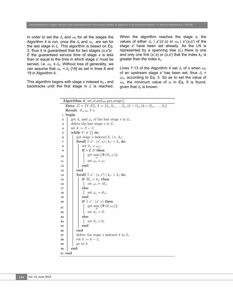
In order to set the Gs and Zs for all the stages the Algorithm 4 is run, once the Gs and Zs are set for the last stage in L. This algorithm is based on Eq. 3, thus it is guaranteed that for two stages (s,s')� E the guaranteed service time of stage s is less than or equal to the time in which stage s' must be served, i.e. Zs � Gs’. Without loss of generality, we can assume that Zs = Gs’ [19] as set in lines 8 and 19 in Algorithm 4. This algorithm begins with stage s indexed kS-1 and backtracks until the first stage in L is reached.

When the algorithm reaches the stage s, the values of either Gs' | s':(s',s) or Zs' | s':(s,s') of the stage s' have been set already. As the LN is represented by a spanning tree (L) there is one and only one link (s',s) or (s,s') that the index ks' is greater than the index ks. Lines 7-13 of the Algorithm 4 set Gs of s when Zs' of an upstream stage s' has been set, thus Gs = Zs', according to Eq. 3. So as to set the value of Zs, the minimum value of Z in Eq. 6 is found, given that Gs is known.



Lines 14–26, set Ȧs once the ࢡs ƍ | sƍ : (s, sƍ) is known. When Ms > ࢡs ƍ , there is no need to place safety stock because the downstream stage s' could wait enough to be served. In this case Ȧs = Ms (line 16), otherwise line 18 is used. To set is found given that w ࢡ s, the minimum value ofࢡ= ws (Eq. 6). If stage s does not have any upstream stage ࢡs = 0 (line 24 If stage s does not have any upstream stage ࢡs = 0 (line 24). Finally, line 27 deletes the stage s which has just been set Ȧs and ࢡs , line 28 deletes the current stage, and line 29 sends the algorithm to evaluate if there are more stages that required their times to be set.

5. Real-life Application The study of a real-life application was carried out in a manufacturing plant that assembles fixed brakes and clutch pedals modules. The company is located in the business automotive cluster in Northeast Mexico and assembles 24 different models, even though we selected the model with the highest sales volume. The LN of the model is depicted in Fig. 2 and the related data is shown in Even though the data in Table 1 have been modified as requested by the company, the LN is the current one and the results and conclusion drawn from this study are acceptable.

Figure 2. Real-life Logistic Network.


Vol.�12,�June�2014�546�

The manufacturing process of the brake pedal comprises a phase of pre-assembly and a phase of assembly. In the pre-assembly phase, the components, supplied at the delivering stages, are welded to each other to go to the next phase. The main components are the switch flag, the arm, the plate, and the main bracket. The switch flag is produced by pressing a roll of steel according to the required length. The plate is produced in the same way the switch flag is, except for the length of the piece and the steel thickness. The arm and the main bracket are produced when a stamped piece is folded.

In the assembly phase, the arm, the plate and the switch flag are welded to each other, then painted by an external provider. Intermediately, after this the painted piece and main plate are taken to the assembly shop. There, the bushes and pivot bolts are inserted into the arm, the plate, and the flag. Then the pedal pad is assembled and the bolts/screws are adjusted according to the desired torque.

Finally, a functional test is carried out and the assembly is labelled, packed, and sent to warehouse ready to be shipped.

stage (s) name

cost(cs)

time(ts)

stage(s) name

cost (cs)

time(ts)

1 99664 11.7 15 34 Yoke RH 29.6 02 99657 34.6 10 35 285567 0.9 603 Cutting 0.4 0 36 Yoke LH 11.4 04 99658 10.6 10 37 285555 0.7 305 285627 1.1 30 38 285591 1.6 406 285635 12.7 30 39 285549 0.9 357 293852 4.3 75 40 Support-Clevis Union 1.4 08 99662 4.0 15 41 Cutting 0.4 09 Cutting 0.5 0 42 Cutting 2.6 1210 Folding 1.5 0 43 Painting 2.4 011 Cutting 0.4 0 44 Yoke RH Bushing Insertion 3.7 012 Worm Shaft Housing

U i0.5 0 45 285529 0.9 35

13 285675 3.5 45 46 Yoke LH Transmission Shaft 4.2 014 285667 11.9 60 47 Folding 1.9 015 285691 9.5 40 48 Cutting 0.2 016 Cutting 0.3 0 49 Arm Yokes Union 4.3 017 Folding 3.0 0 50 285514 0.8 4018 Yoke RH 13.7 0 51 285603 0.7 4019 Leveler 11.1 0 52 285519 7.9 3020 99663 10.9 12 53 Welding 4.1 021 285643 0.4 55 54 Clevis Bolt Insertion 3.3 022 285651 0.3 65 55 293482 4.9 6023 285611 0.4 30 56 291026 25.7 5524 Transmission Housing

U i0.7 0 57 Main Bracket 32.7 0

25 285619 0.8 70 58 287723 3.0 5026 285659 0.3 30 59 285552 0.7 8027 Plate 4.4 0 60 Pedal Pad Insertion 1.2 028 Arm 38.0 0 61 Pivot Bolt Insertion 1.8 029 Welding 4.8 0 62 Functional Tests 0.8 030 Cutting 0.4 0 63 Packing 0.9 031 99675 23.6 10 64 Shipping 0.7 032 Welding 4.8 0 65 T1ADJ 238.9 033 285585 1.1 40

Table 1. Data of the Real-life Application.



Based on historical demand, we set the value of demand and standard deviation to Ps�D=32'500$ and Vs�D = 534$ units per day. The safety factor per stage is ks =1.645 and the unit holding cost is h=0.2 . The algorithm was run in a Lenovo T520 computer with an Intel Core i5 processor at 2.5GHz and 4GB in RAM memory 6. Results One of the most important issues in the guaranteed-service time inventory models is the cost of safety stock for a given guaranteed-service time (:) in the delivering stages. Hence, we run the algorithm by setting :=0,10,20,…,100 as shown in Figure 3. According to it, the maximum safety stock is $171'110 when the guaranteed-service time is set to zero, i.e. :=0. We can see from Figure 3 that the shorter the guaranteed-service time, the higher the safety stock cost. In our real-life logistic network (Figure 2), the safety stock cost is lower when the :�is increased from 0 to 40 days. After that, the cost remains constant ($40'863$) until :=80 days, i.e. Zs d 40 even though :�= (40,80), see constraint 4. If we set :�80, the safety stock cost is zero

because of the maximum replenishment time of the last stage s65, see Table 2. In this case, there is no need to keep safety stock. In Table 2, columns 1, 2, and 3 are common for all the values of :. The data shown in columns 4,5,6, and 7 are computed when :�= 40. As shown in columns 4 and 5, the values of the Gs for the stages when ts = 0 is equal to and Zs, so the days of inventory Us are zero, thus these stages do not hold any inventory. On the other hand, in eleven stages there is need to stock inventory because the large times ts, see Table 2. The largest one is t59=80 days, thus the days of inventory is set to U59=40. Stage s59 represents a component named 285552 which is brought from overseas. The long-time affects the position of inventory of the successive stages because the time in which those stages perform their task is zero.

Although the company must hold 40 days of inventory of the component 285552, its safety stock cost is not the highest one. Component 291026 (s56 ) holds 10 days of inventory with a cost of $17'434, thus the company decided to implement a more tight control over this component.

Figure 3. Safety Stock costs for different values of � (Eq. 4).


Vol.�12,�June�2014�548�

stage (s)

Cumulative cost (Cs)

Max. replenishment time (Ms)

sࢡ

Ȧs

Days of inventory (Us)

Inventory cost

1 11.7 15 0 15 0 0 2 34.6 10 0 10 0 0 3 12.1 15 15 15 0 0 4 10.6 10 0 10 0 0 5 1.1 30 0 30 0 0 6 12.7 30 0 30 0 0 7 4.3 75 0 40 35 4’456 8 4.0 15 0 15 0 0 9 35.1 10 10 10 0 0

10 13.6 15 15 15 0 0 11 11.0 10 10 10 0 0 12 18.6 75 40 40 0 0 13 3.5 45 0 40 5 1’371 14 11.9 60 0 40 20 9’321 15 9.5 40 0 40 0 0 16 4.3 15 15 15 0 0 17 38.1 10 10 10 0 0 18 27.3 15 15 15 0 0 19 22.1 10 10 10 0 0 20 10.9 12 0 12 0 0 21 0.4 55 0 40 15 271 22 0.3 65 0 40 25 263 23 0.4 30 0 30 0 0 24 44.2 75 40 40 0 0 25 0.8 70 0 40 30 767 26 0.3 30 0 30 0 0 27 8.7 15 15 15 0 0 28 76.1 10 10 10 0 0 29 54.2 15 15 15 0 0 30 11.3 12 12 12 0 0 31 23.6 10 0 10 0 0 32 89.6 15 15 15 0 0 33 1.1 40 0 40 0 0 34 83.8 15 15 15 0 0 35 0.9 60 0 40 20 705 36 22.7 12 12 12 0 0 37 0.7 30 0 30 0 0 38 1.6 40 0 40 0 0 39 0.9 35 0 35 0 0 40 47.8 75 40 40 0 0 41 24.0 10 10 10 0 0 42 2.6 12 0 12 0 0 43 92.0 15 15 15 0 0 44 88.6 40 40 40 0 0 45 0.9 35 0 35 0 0 46 78.8 75 40 40 0 0 47 25.9 10 10 10 0 0 48 2.8 12 12 12 0 0 49 264.6 75 40 40 0 0 50 0.8 40 0 40 0 0 51 0.7 40 0 40 0 0 52 7.9 30 0 30 0 0 53 32.8 12 12 12 0 0 54 277.3 75 40 40 0 0 55 4.9 60 0 40 20 3’838 56 25.7 55 0 40 15 17’434 57 65.5 12 12 12 0 0 58 3.0 50 0 40 10 1’662 59 0.7 80 0 40 40 775 60 309.1 75 40 40 0 0 61 380.1 80 40 40 0 0 62 380.9 80 40 40 0 0 63 381.8 80 40 40 0 0 64 382.5 80 40 40 0 0 65 621.4 80 40 40 0 0

Table 2. Total safety stock when � = 40.



7. Conclusions In this paper, we solved a real-life application of a company that assembles fixed brakes and clutch pedals. We applied the dynamic programming algorithm developed in [2] and we proposed a framework to solve mid-size logistic networks (see Figure 1). The framework is based on a Java application called JbA. We provide the pseudo code of the algorithm to place safety stock inventory in guaranteed service time models. The JbA solved a 65-stage logistic network in about 341ms, thus the implemented algorithm solved it efficiently. According to the company, it holds four weeks of safety stock for most of the components and assemblies. After the JbA is run, we conclude that most of the stages do not hold inventory as shown in Table 2 and just stages s7, s25, and s59 require safety stock for about 4 weeks. Future extensions of this algorithm must be implemented in real-life applications. Some exertions include stochastic times, non-stationary demand and capacity constraints. Moreover, there is a need for develop algorithms based on new optimisation techniques given that the guaranteed-service inventory models has been proven to be NP-hard.

References [1] Lee, H., Padmanabhan, V. & Whang, S., Information distortion in a supply chain: the bullwhip effect, Management Science, Vol. 43, No. 4, 1997, pp. 546–558. [2] Graves, S. & Willems, S., Optimizing strategic safety stock placement in supply chains, Manufacturing & Service Operations Management, Vol. 2, No. 1, 2000, pp. 68–83. [3] Snyder, L.V. & Shen, Z.J.M., Fundamentals of Supply Chain Theory. Wiley, 2011, pp 367. [4] Glasserman, P. & Tayur, S., Sensitivity analysis for base-stock levels in multi-echelon production-inventory systems, Management Science, Vol. 41, 1995, pp. 263–281. [5] Levner, E., Perlman, Y., & Cheng, T.C.E. & Levner, I, A network approach to modeling the multi-echelon spare-part inventory system with backorders and interval-valued demand, International Journal of Production Economics, vol. 132, no. 1, 2011, pp. 43-51. [6] Simpson, K., In-process inventories, Operations Research, Vol. 6, No. 6, 1958, pp. 863–873. [7] Graves, S., Safety stocks in manufacturing systems, Journal of Manufacturing and Operations Management, Vol. 1, No. 1, 1988, pp. 67–101. [8] Inderfurth, K., Safety stock optimization in multi-stage inventory systems, International Journal of Production Economics, Vol. 24, No. 1, 1991, pp. 103–113. [9] Inderfurth, K, & Minner, S., Safety stocks in multi-stage inventory systems under different service measures, European Journal of Operational Research, Vol. 106, No. 1, pp. 57 – 73. [10] Graves, S. & Willems, S., Strategic safety stock placement in supply chains, in Proceedings of 1996 MSOM, 1996, pp 299 -304, Dartmouth, Hannover, USA, July. [11] Graves, S. & Willems, S., Supply chain design: safety stock placement and supply chain configuration, in Handbooks in Operations Research and Management Science, A. G. de Kok and S. Graves Editors, Elsevier, 2003, pp. 95–132. [12] Lesnaia, E., Vasilescu, I., & Graves, S., The complexity of safety stock placement in general-network supply chains, Innovation in Manufacturing Systems and Technology (IMST), 2005.


Vol.�12,�June�2014�550�

[13] Lesnaia, E., Optimizing safety stock placement in general network supply chains, PhD thesis, MIT, 2004. [14] Magnanti, T., Shen, Z., Shu, J., Simchi-Levi, D. & Teo, C., Inventory placement in acyclic supply chain networks, Operations Research Letters, Vol. 34, No. 2, 2006, pp. 228 – 238. [15] Graves S. & Lesnaia, E., Optimizing safety stock placement in general network supply chains, in Proceedings of Singapore-MIT Alliance Annual Symposium Conference, 2004, pp. 7–13, 2004, Singapore. [16] Shu J. &. Karimi, I., Efficient heuristics for inventory placement in acyclic net319 works, Computers & Operations Research, Vol. 36, No. 11, 2009, pp. 2899 – 2904. [17] Huang, G., Zhang, X. & Liang, L., Towards integrated optimal configuration of platform products, manufacturing processes, and supply chains, Journal of Operations Management, Vol. 23, No. 3-4, 2005, pp. 267–290. [18] Schoenmeyr, T. & Graves, S., Strategic safety stocks in supply chains with capacity constraints, tech. rep., Massachusetts Institute of Technology, 2009. [19] Graves, S. & Willems, S., Optimizing the supply chain configuration for new products, Management Science, Vol. 51, No. 8, 2005, pp. 1165–1180. [20] Graves, S. & Willems, S., Strategic inventory placement in supply chains: Nonstationary demand, Manufacturing & Service Operations Management, Vol. 10, No. 2, 2008, pp. 278–287. [21] Humair, S., Ruark, J., Tomlin, B. & Willems, S., Incorporating stochastic lead times into the guaranteed service model of safety stock optimization, 2012. [22] Hegge, H. & Wortmann, J., Generic bill-of-material: a new product model, International Journal of Production Economics, Vol. 23, No. 1–3, 1991, pp. 117 – 128. [23] Elizondo-Cortés, M. & Aceves-García, R., Strategy of solution for the inventory routing problem based on separable cross decomposition, Journal of Applied Research and Technology, Vol. 3, No 2, 2005, pp 139-149. [24] Cedillo-Campos, M. & Sánchez-Ramírez, R., Dynamic Self-Assessment of Supply Chains Performance: an Emerging Market Approach, Journal of Applied Research and Technology, Vol. 11, No 3, 2013, pp 338-347.

[25] Fathollah, M., Taham, F. & Ashouri, A., Developing a Conceptual Framework for Simulation Analysis in a Supply Chain Based on Common Platform (SCBCP), Journal of Applied Research and Technology, Vol. 7, No 2, pp 163-184. [26] González-Ramírez, R.G., Smith, N. R., Askin, R. G., Miranda, Pablo A. & Sánchez, J.M., A Hybrid Metaheuristic Approach to Optimize the Districting Design of a Parcel Company, Journal of Applied Research and Technology, Vol. 9, No 1, 2011, pp 19-35 ��

�

Documents

18 placing safety - SciELO · The aim of this paper is to solve the problem of placing safety stock over a Logistic Network (LN) that is represented by a Generic Bill of Materials