Embed Size (px)
Citation preview
18.600: Lecture 36
Risk Neutral Probability and Black-Scholes
Scott Sheffield
MIT
18.600 Lecture 36

Outline
Risk neutral probability
Black-Scholes
18.600 Lecture 36
Outline
Risk neutral probability
Black-Scholes
18.600 Lecture 36

Overview
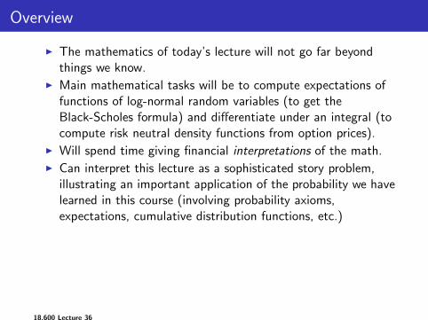
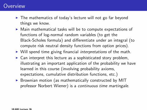
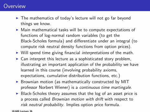
I The mathematics of today’s lecture will not go far beyondthings we know.
I Main mathematical tasks will be to compute expectations offunctions of log-normal random variables (to get theBlack-Scholes formula) and differentiate under an integral (tocompute risk neutral density functions from option prices).
I Will spend time giving financial interpretations of the math.I Can interpret this lecture as a sophisticated story problem,
illustrating an important application of the probability we havelearned in this course (involving probability axioms,expectations, cumulative distribution functions, etc.)
I Brownian motion (as mathematically constructed by MITprofessor Norbert Wiener) is a continuous time martingale.
I Black-Scholes theory assumes that the log of an asset price isa process called Brownian motion with drift with respect torisk neutral probability. Implies option price formula.
18.600 Lecture 36
Overview
I The mathematics of today’s lecture will not go far beyondthings we know.
I Main mathematical tasks will be to compute expectations offunctions of log-normal random variables (to get theBlack-Scholes formula) and differentiate under an integral (tocompute risk neutral density functions from option prices).
I Will spend time giving financial interpretations of the math.
I Can interpret this lecture as a sophisticated story problem,illustrating an important application of the probability we havelearned in this course (involving probability axioms,expectations, cumulative distribution functions, etc.)
I Brownian motion (as mathematically constructed by MITprofessor Norbert Wiener) is a continuous time martingale.
I Black-Scholes theory assumes that the log of an asset price isa process called Brownian motion with drift with respect torisk neutral probability. Implies option price formula.
18.600 Lecture 36
Overview
I The mathematics of today’s lecture will not go far beyondthings we know.
I Main mathematical tasks will be to compute expectations offunctions of log-normal random variables (to get theBlack-Scholes formula) and differentiate under an integral (tocompute risk neutral density functions from option prices).
I Will spend time giving financial interpretations of the math.I Can interpret this lecture as a sophisticated story problem,
illustrating an important application of the probability we havelearned in this course (involving probability axioms,expectations, cumulative distribution functions, etc.)
I Brownian motion (as mathematically constructed by MITprofessor Norbert Wiener) is a continuous time martingale.
I Black-Scholes theory assumes that the log of an asset price isa process called Brownian motion with drift with respect torisk neutral probability. Implies option price formula.
18.600 Lecture 36
Overview
I The mathematics of today’s lecture will not go far beyondthings we know.
I Main mathematical tasks will be to compute expectations offunctions of log-normal random variables (to get theBlack-Scholes formula) and differentiate under an integral (tocompute risk neutral density functions from option prices).
I Will spend time giving financial interpretations of the math.I Can interpret this lecture as a sophisticated story problem,
illustrating an important application of the probability we havelearned in this course (involving probability axioms,expectations, cumulative distribution functions, etc.)
I Brownian motion (as mathematically constructed by MITprofessor Norbert Wiener) is a continuous time martingale.
I Black-Scholes theory assumes that the log of an asset price isa process called Brownian motion with drift with respect torisk neutral probability. Implies option price formula.
18.600 Lecture 36

See desk at office hours
18.600 Lecture 36
Risk neutral probability
I “Risk neutral probability” is a fancy term for “priceprobability”. (The term “price probability” is arguably moredescriptive.)
I That is, it is a probability measure that you can deduce bylooking at prices.
I For example, suppose somebody is about to shoot a freethrow in basketball. What is the price in the sports bettingworld of a contract that pays one dollar if the shot is made?
I If the answer is .75 dollars, then we say that the risk neutralprobability that the shot will be made is .75.
I Risk neutral probability is the probability determined by themarket betting odds.
18.600 Lecture 36
Risk neutral probability of outcomes known at fixed time T
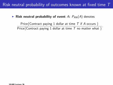
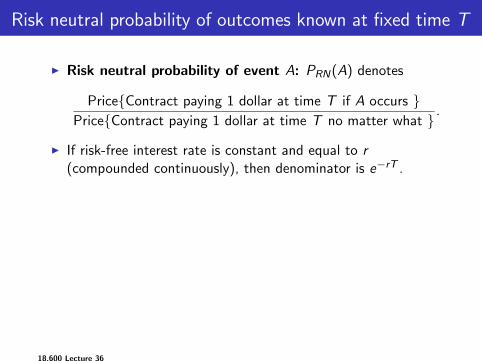
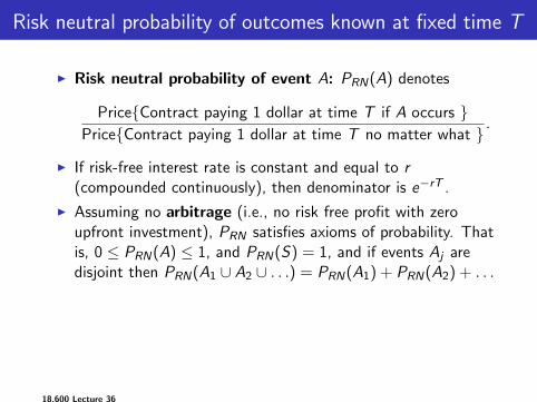
I Risk neutral probability of event A: PRN(A) denotes
Price{Contract paying 1 dollar at time T if A occurs }Price{Contract paying 1 dollar at time T no matter what } .
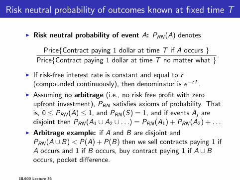
I If risk-free interest rate is constant and equal to r(compounded continuously), then denominator is e−rT .
I Assuming no arbitrage (i.e., no risk free profit with zeroupfront investment), PRN satisfies axioms of probability. Thatis, 0 ≤ PRN(A) ≤ 1, and PRN(S) = 1, and if events Aj aredisjoint then PRN(A1 ∪ A2 ∪ . . .) = PRN(A1) + PRN(A2) + . . .
I Arbitrage example: if A and B are disjoint andPRN(A ∪ B) < P(A) + P(B) then we sell contracts paying 1 ifA occurs and 1 if B occurs, buy contract paying 1 if A ∪ Boccurs, pocket difference.
18.600 Lecture 36
Risk neutral probability of outcomes known at fixed time T
I Risk neutral probability of event A: PRN(A) denotes
Price{Contract paying 1 dollar at time T if A occurs }Price{Contract paying 1 dollar at time T no matter what } .
I If risk-free interest rate is constant and equal to r(compounded continuously), then denominator is e−rT .
I Assuming no arbitrage (i.e., no risk free profit with zeroupfront investment), PRN satisfies axioms of probability. Thatis, 0 ≤ PRN(A) ≤ 1, and PRN(S) = 1, and if events Aj aredisjoint then PRN(A1 ∪ A2 ∪ . . .) = PRN(A1) + PRN(A2) + . . .
I Arbitrage example: if A and B are disjoint andPRN(A ∪ B) < P(A) + P(B) then we sell contracts paying 1 ifA occurs and 1 if B occurs, buy contract paying 1 if A ∪ Boccurs, pocket difference.
18.600 Lecture 36
Risk neutral probability differ vs. “ordinary probability”
I At first sight, one might think that PRN(A) describes themarket’s best guess at the probability that A will occur.
I But suppose A is the event that the government is dissolvedand all dollars become worthless. What is PRN(A)?
I Should be 0. Even if people think A is likely, a contractpaying a dollar when A occurs is worthless.
I Now, suppose there are only 2 outcomes: A is event thateconomy booms and everyone prospers and B is event thateconomy sags and everyone is needy. Suppose purchasingpower of dollar is the same in both scenarios. If people thinkA has a .5 chance to occur, do we expect PRN(A) > .5 orPRN(A) < .5?
I Answer: PRN(A) < .5. People are risk averse. In secondscenario they need the money more.
18.600 Lecture 36
Non-systemic event
I Suppose that A is the event that the Boston Red Sox win theWorld Series. Would we expect PRN(A) to represent (themarket’s best assessment of) the probability that the Red Soxwill win?
I Arguably yes. The amount that people in general need orvalue dollars does not depend much on whether A occurs(even though the financial needs of specific individuals maydepend on heavily on A).
I Even if some people bet based on loyalty, emotion, insuranceagainst personal financial exposure to team’s prospects, etc.,there will arguably be enough in-it-for-the-money statisticalarbitrageurs to keep price near a reasonable guess of whatwell-informed informed experts would consider the trueprobability.
18.600 Lecture 36
Extensions of risk neutral probability
I Definition of risk neutral probability depends on choice ofcurrency (the so-called numeraire).
I Risk neutral probability can be defined for variable times andvariable interest rates — e.g., one can take the numeraire tobe amount one dollar in a variable-interest-rate money marketaccount has grown to when outcome is known. Can definePRN(A) to be price of contract paying this amount if andwhen A occurs.
I For simplicity, we focus on fixed time T , fixed interest rate rin this lecture.
18.600 Lecture 36
Risk neutral probability is objective
I Check out binary prediction contracts at predictwise.com,oddschecker.com, predictit.com, etc.
I Many financial derivatives are essentially bets of this form.
I Unlike “true probability” (what does that mean?) the “riskneutral probability” is an objectively measurable price.
I Pundit: The market predictions are ridiculous. I can estimateprobabilities much better than they can.
I Listener: Then why not make some bets and get rich? If yourestimates are so much better, law of large numbers says you’llsurely come out way ahead eventually.
I Pundit: Well, you know... been busy... scruples aboutgambling... more to life than money...
I Listener: Yeah, that’s what I thought.
18.600 Lecture 36
Prices as expectations
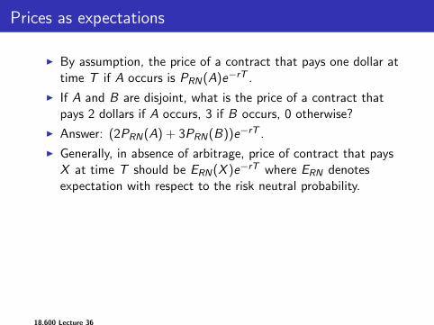
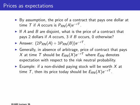
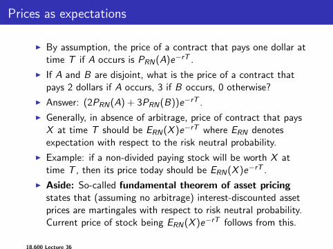
I By assumption, the price of a contract that pays one dollar attime T if A occurs is PRN(A)e−rT .
I If A and B are disjoint, what is the price of a contract thatpays 2 dollars if A occurs, 3 if B occurs, 0 otherwise?
I Answer: (2PRN(A) + 3PRN(B))e−rT .
I Generally, in absence of arbitrage, price of contract that paysX at time T should be ERN(X )e−rT where ERN denotesexpectation with respect to the risk neutral probability.
I Example: if a non-divided paying stock will be worth X attime T , then its price today should be ERN(X )e−rT .
I Aside: So-called fundamental theorem of asset pricingstates that (assuming no arbitrage) interest-discounted assetprices are martingales with respect to risk neutral probability.Current price of stock being ERN(X )e−rT follows from this.
18.600 Lecture 36
Prices as expectations
I By assumption, the price of a contract that pays one dollar attime T if A occurs is PRN(A)e−rT .
I If A and B are disjoint, what is the price of a contract thatpays 2 dollars if A occurs, 3 if B occurs, 0 otherwise?
I Answer: (2PRN(A) + 3PRN(B))e−rT .
I Generally, in absence of arbitrage, price of contract that paysX at time T should be ERN(X )e−rT where ERN denotesexpectation with respect to the risk neutral probability.
I Example: if a non-divided paying stock will be worth X attime T , then its price today should be ERN(X )e−rT .
I Aside: So-called fundamental theorem of asset pricingstates that (assuming no arbitrage) interest-discounted assetprices are martingales with respect to risk neutral probability.Current price of stock being ERN(X )e−rT follows from this.
18.600 Lecture 36
Outline
Risk neutral probability
Black-Scholes
18.600 Lecture 36
Outline
Risk neutral probability
Black-Scholes
18.600 Lecture 36
Black-Scholes: main assumption and conclusion
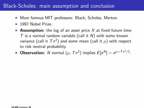
I More famous MIT professors: Black, Scholes, Merton.
I 1997 Nobel Prize.
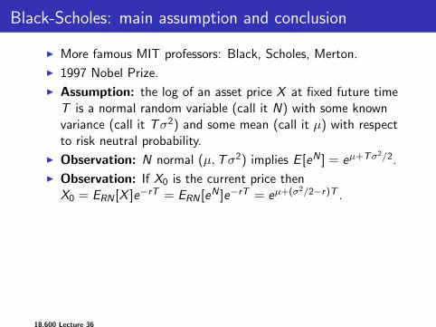
I Assumption: the log of an asset price X at fixed future timeT is a normal random variable (call it N) with some knownvariance (call it Tσ2) and some mean (call it µ) with respectto risk neutral probability.
I Observation: N normal (µ,Tσ2) implies E [eN ] = eµ+Tσ2/2.
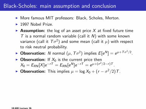
I Observation: If X0 is the current price thenX0 = ERN [X ]e−rT = ERN [eN ]e−rT = eµ+(σ2/2−r)T .
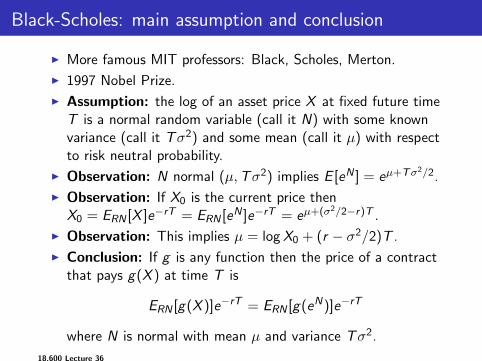
I Observation: This implies µ = logX0 + (r − σ2/2)T .
I Conclusion: If g is any function then the price of a contractthat pays g(X ) at time T is
ERN [g(X )]e−rT = ERN [g(eN)]e−rT
where N is normal with mean µ and variance Tσ2.
18.600 Lecture 36
Black-Scholes: main assumption and conclusion
I More famous MIT professors: Black, Scholes, Merton.
I 1997 Nobel Prize.
I Assumption: the log of an asset price X at fixed future timeT is a normal random variable (call it N) with some knownvariance (call it Tσ2) and some mean (call it µ) with respectto risk neutral probability.
I Observation: N normal (µ,Tσ2) implies E [eN ] = eµ+Tσ2/2.
I Observation: If X0 is the current price thenX0 = ERN [X ]e−rT = ERN [eN ]e−rT = eµ+(σ2/2−r)T .
I Observation: This implies µ = logX0 + (r − σ2/2)T .
I Conclusion: If g is any function then the price of a contractthat pays g(X ) at time T is
ERN [g(X )]e−rT = ERN [g(eN)]e−rT
where N is normal with mean µ and variance Tσ2.
18.600 Lecture 36
Black-Scholes example: European call option
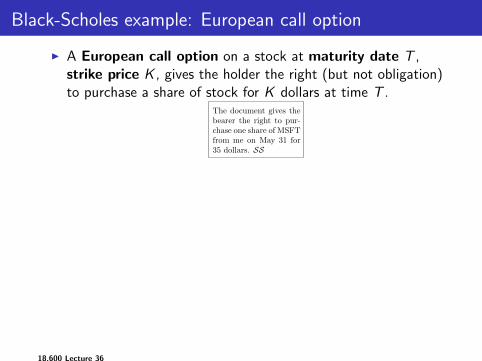
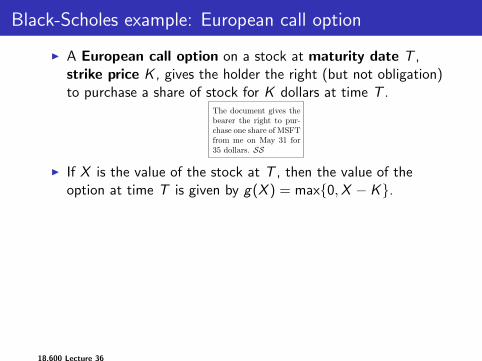
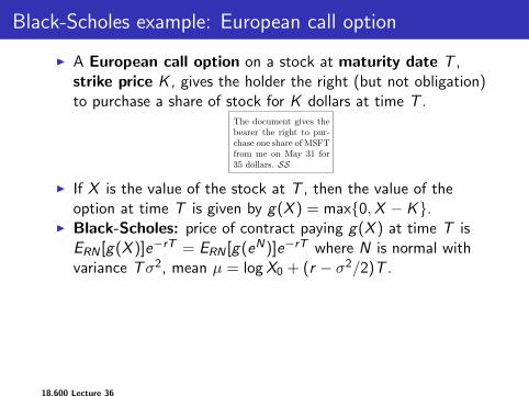
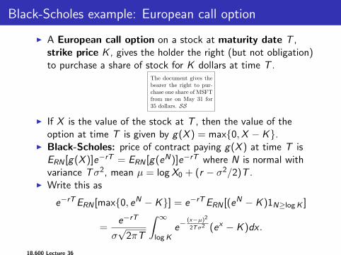
I A European call option on a stock at maturity date T ,strike price K , gives the holder the right (but not obligation)to purchase a share of stock for K dollars at time T .
The document gives thebearer the right to pur-chase one share of MSFTfrom me on May 31 for35 dollars. SS
I If X is the value of the stock at T , then the value of theoption at time T is given by g(X ) = max{0,X − K}.
I Black-Scholes: price of contract paying g(X ) at time T isERN [g(X )]e−rT = ERN [g(eN)]e−rT where N is normal withvariance Tσ2, mean µ = logX0 + (r − σ2/2)T .
I Write this as
e−rTERN [max{0, eN − K}] = e−rTERN [(eN − K )1N≥logK ]
=e−rT
σ√
2πT
∫ ∞logK
e−(x−µ)2
2Tσ2 (ex − K )dx .
18.600 Lecture 36
Black-Scholes example: European call option
I A European call option on a stock at maturity date T ,strike price K , gives the holder the right (but not obligation)to purchase a share of stock for K dollars at time T .
The document gives thebearer the right to pur-chase one share of MSFTfrom me on May 31 for35 dollars. SS
I If X is the value of the stock at T , then the value of theoption at time T is given by g(X ) = max{0,X − K}.
I Black-Scholes: price of contract paying g(X ) at time T isERN [g(X )]e−rT = ERN [g(eN)]e−rT where N is normal withvariance Tσ2, mean µ = logX0 + (r − σ2/2)T .
I Write this as
e−rTERN [max{0, eN − K}] = e−rTERN [(eN − K )1N≥logK ]
=e−rT
σ√
2πT
∫ ∞logK
e−(x−µ)2
2Tσ2 (ex − K )dx .
18.600 Lecture 36
The famous formula
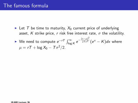
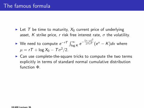
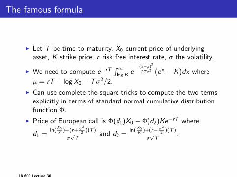
I Let T be time to maturity, X0 current price of underlyingasset, K strike price, r risk free interest rate, σ the volatility.
I We need to compute e−rT∫∞logK e−
(x−µ)2
2Tσ2 (ex − K )dx where
µ = rT + logX0 − Tσ2/2.
I Can use complete-the-square tricks to compute the two termsexplicitly in terms of standard normal cumulative distributionfunction Φ.
I Price of European call is Φ(d1)X0 − Φ(d2)Ke−rT where
d1 =ln(
X0K)+(r+σ2
2)(T )
σ√T
and d2 =ln(
X0K)+(r−σ2
2)(T )
σ√T
.
18.600 Lecture 36
The famous formula
I Let T be time to maturity, X0 current price of underlyingasset, K strike price, r risk free interest rate, σ the volatility.
I We need to compute e−rT∫∞logK e−
(x−µ)2
2Tσ2 (ex − K )dx where
µ = rT + logX0 − Tσ2/2.
I Can use complete-the-square tricks to compute the two termsexplicitly in terms of standard normal cumulative distributionfunction Φ.
I Price of European call is Φ(d1)X0 − Φ(d2)Ke−rT where
d1 =ln(
X0K)+(r+σ2
2)(T )
σ√T
and d2 =ln(
X0K)+(r−σ2
2)(T )
σ√T
.
18.600 Lecture 36
Determining risk neutral probability from call quotes
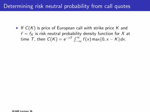
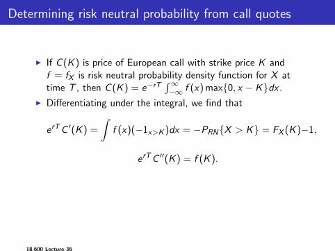
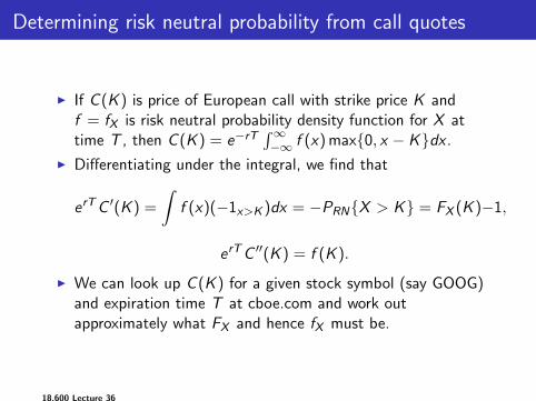
I If C (K ) is price of European call with strike price K andf = fX is risk neutral probability density function for X attime T , then C (K ) = e−rT
∫∞−∞ f (x) max{0, x − K}dx .
I Differentiating under the integral, we find that
erTC ′(K ) =
∫f (x)(−1x>K )dx = −PRN{X > K} = FX (K )−1,
erTC ′′(K ) = f (K ).
I We can look up C (K ) for a given stock symbol (say GOOG)and expiration time T at cboe.com and work outapproximately what FX and hence fX must be.
18.600 Lecture 36
Determining risk neutral probability from call quotes
I If C (K ) is price of European call with strike price K andf = fX is risk neutral probability density function for X attime T , then C (K ) = e−rT
∫∞−∞ f (x) max{0, x − K}dx .
I Differentiating under the integral, we find that
erTC ′(K ) =
∫f (x)(−1x>K )dx = −PRN{X > K} = FX (K )−1,
erTC ′′(K ) = f (K ).
I We can look up C (K ) for a given stock symbol (say GOOG)and expiration time T at cboe.com and work outapproximately what FX and hence fX must be.
18.600 Lecture 36
Perspective: implied volatility
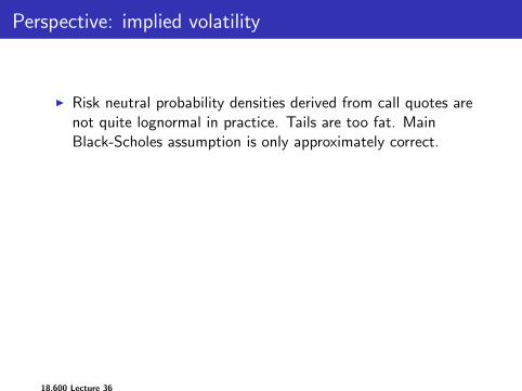
I Risk neutral probability densities derived from call quotes arenot quite lognormal in practice. Tails are too fat. MainBlack-Scholes assumption is only approximately correct.
I “Implied volatility” is the value of σ that (when plugged intoBlack-Scholes formula along with known parameters) predictsthe current market price.
I If Black-Scholes were completely correct, then given a stockand an expiration date, the implied volatility would be thesame for all strike prices. In practice, when the impliedvolatility is viewed as a function of strike price (sometimescalled the “volatility smile”), it is not constant.
18.600 Lecture 36
Perspective: implied volatility
I Risk neutral probability densities derived from call quotes arenot quite lognormal in practice. Tails are too fat. MainBlack-Scholes assumption is only approximately correct.
I “Implied volatility” is the value of σ that (when plugged intoBlack-Scholes formula along with known parameters) predictsthe current market price.
I If Black-Scholes were completely correct, then given a stockand an expiration date, the implied volatility would be thesame for all strike prices. In practice, when the impliedvolatility is viewed as a function of strike price (sometimescalled the “volatility smile”), it is not constant.
18.600 Lecture 36
Perspective: why is Black-Scholes not exactly right?
I Main Black-Scholes assumption: risk neutral probabilitydensities are lognormal.
I Heuristic support for this assumption: If price goes up 1percent or down 1 percent each day (with no interest) thenthe risk neutral probability must be .5 for each (independentlyof previous days). Central limit theorem gives log normalityfor large T .
I Replicating portfolio point of view: in the simple binarytree models (or continuum Brownian models), we can transfermoney back and forth between the stock and the risk freeasset to ensure our wealth at time T equals the option payout.Option price is required initial investment, which is risk neutralexpectation of payout. “True probabilities” are irrelevant.
I Where arguments for assumption break down: Fluctuationsizes vary from day to day. Prices can have big jumps.
I Fixes: variable volatility, random interest rates, Levy jumps....
18.600 Lecture 36