18.950 (Di erential Geometry) Lecture Notes · 2018-05-09 · Evan Chen (Fall 2015) 18.950 (Di erential Geometry) Lecture Notes §1September 10, 2015 Here is an intuitive sketch of

18.950 (Differential Geometry) Lecture Notes

Evan Chen

Fall 2015

This is MIT’s undergraduate 18.950, instructed by Xin Zhou. The formalname for this class is “Differential Geometry”.

The permanent URL for this document is http://web.evanchen.cc/

coursework.html, along with all my other course notes.

Contents

1 September 10, 2015 31.1 Curves . . . . . . . . . . . . . . . . . . . . . . . . . . . . . . . . . . . . . . 31.2 Surfaces . . . . . . . . . . . . . . . . . . . . . . . . . . . . . . . . . . . . . 31.3 Parametrized Curves . . . . . . . . . . . . . . . . . . . . . . . . . . . . . . 4

2 September 15, 2015 52.1 Regular curves . . . . . . . . . . . . . . . . . . . . . . . . . . . . . . . . . 52.2 Arc Length Parametrization . . . . . . . . . . . . . . . . . . . . . . . . . . 62.3 Change of Orientation . . . . . . . . . . . . . . . . . . . . . . . . . . . . . 72.4 Vector Product in R3 . . . . . . . . . . . . . . . . . . . . . . . . . . . . . 72.5 OH GOD NO . . . . . . . . . . . . . . . . . . . . . . . . . . . . . . . . . . 72.6 Concrete examples . . . . . . . . . . . . . . . . . . . . . . . . . . . . . . . 8

3 September 17, 2015 93.1 Always Cauchy-Schwarz . . . . . . . . . . . . . . . . . . . . . . . . . . . . 93.2 Curvature . . . . . . . . . . . . . . . . . . . . . . . . . . . . . . . . . . . . 93.3 Torsion . . . . . . . . . . . . . . . . . . . . . . . . . . . . . . . . . . . . . 93.4 Frenet formulas . . . . . . . . . . . . . . . . . . . . . . . . . . . . . . . . . 103.5 Convenient Formulas . . . . . . . . . . . . . . . . . . . . . . . . . . . . . . 11

4 September 22, 2015 124.1 Signed Curvature . . . . . . . . . . . . . . . . . . . . . . . . . . . . . . . . 124.2 Evolute of a Curve . . . . . . . . . . . . . . . . . . . . . . . . . . . . . . . 124.3 Isoperimetric Inequality . . . . . . . . . . . . . . . . . . . . . . . . . . . . 13

5 September 24, 2015 155.1 Regular Surfaces . . . . . . . . . . . . . . . . . . . . . . . . . . . . . . . . 155.2 Special Cases of Manifolds . . . . . . . . . . . . . . . . . . . . . . . . . . 15

6 September 29, 2015 and October 1, 2015 176.1 Local Parametrizations . . . . . . . . . . . . . . . . . . . . . . . . . . . . 176.2 Differentiability . . . . . . . . . . . . . . . . . . . . . . . . . . . . . . . . . 176.3 The Tangent Map . . . . . . . . . . . . . . . . . . . . . . . . . . . . . . . 17

1

http://web.evanchen.cc/coursework.html

http://web.evanchen.cc/coursework.html

Evan Chen (Fall 2015) 18.950 (Differential Geometry) Lecture Notes

7 October 6, 2015 197.1 Local Diffeomorphism . . . . . . . . . . . . . . . . . . . . . . . . . . . . . 197.2 Normals to Surfaces . . . . . . . . . . . . . . . . . . . . . . . . . . . . . . 197.3 The First Fundamental Form . . . . . . . . . . . . . . . . . . . . . . . . . 197.4 Relating curves by the first fundamental form . . . . . . . . . . . . . . . . 217.5 Areas . . . . . . . . . . . . . . . . . . . . . . . . . . . . . . . . . . . . . . 22

8 October 8, 2015 and October 15, 2015 238.1 Differentiable Field of Normal Unit Vectors . . . . . . . . . . . . . . . . . 238.2 Second Fundamental Form . . . . . . . . . . . . . . . . . . . . . . . . . . 23

9 October 20, 2015 259.1 Self-Adjoint Maps . . . . . . . . . . . . . . . . . . . . . . . . . . . . . . . 259.2 Line of Curvatures . . . . . . . . . . . . . . . . . . . . . . . . . . . . . . . 259.3 Gauss curvature and Mean Curvature . . . . . . . . . . . . . . . . . . . . 259.4 Gauss Map under Local Coordinates . . . . . . . . . . . . . . . . . . . . . 26

10 October 22, 2015 2710.1 Completing Equations of Weingarten . . . . . . . . . . . . . . . . . . . . . 2710.2 An Example Calculation . . . . . . . . . . . . . . . . . . . . . . . . . . . . 2710.3 Elliptic and Hyperbolic Points . . . . . . . . . . . . . . . . . . . . . . . . 2810.4 Principal Directions . . . . . . . . . . . . . . . . . . . . . . . . . . . . . . 29

11 October 29, 2015 and November 3, 2015 3011.1 Isometries . . . . . . . . . . . . . . . . . . . . . . . . . . . . . . . . . . . . 3011.2 The Christoffel Symbols . . . . . . . . . . . . . . . . . . . . . . . . . . . . 3011.3 Gauss Equations and Mainardi-Codazzi . . . . . . . . . . . . . . . . . . . 3111.4 Bonnet Theorem . . . . . . . . . . . . . . . . . . . . . . . . . . . . . . . . 31

12 November 5, 10, 12, 17, 19 2015 3212.1 The Covariant Derivative . . . . . . . . . . . . . . . . . . . . . . . . . . . 3212.2 Parallel Transports . . . . . . . . . . . . . . . . . . . . . . . . . . . . . . . 3212.3 Geodesics . . . . . . . . . . . . . . . . . . . . . . . . . . . . . . . . . . . . 32

13 November 24 and 26, 2015 3413.1 Area Differential Form . . . . . . . . . . . . . . . . . . . . . . . . . . . . . 3413.2 Global Gauss-Bonnet Theorem . . . . . . . . . . . . . . . . . . . . . . . . 34

14 December 1 and December 3, 2015 3514.1 The Exponential Map . . . . . . . . . . . . . . . . . . . . . . . . . . . . . 3514.2 Local Coordinates . . . . . . . . . . . . . . . . . . . . . . . . . . . . . . . 35

15 December 8 and December 10, 2015 3615.1 Completeness . . . . . . . . . . . . . . . . . . . . . . . . . . . . . . . . . . 3615.2 Variations . . . . . . . . . . . . . . . . . . . . . . . . . . . . . . . . . . . . 3615.3 The Second Variation . . . . . . . . . . . . . . . . . . . . . . . . . . . . . 3715.4 Proof of Bonnet Theorem . . . . . . . . . . . . . . . . . . . . . . . . . . . 38

A Examples 40A.1 Sphere . . . . . . . . . . . . . . . . . . . . . . . . . . . . . . . . . . . . . . 40A.2 Torus . . . . . . . . . . . . . . . . . . . . . . . . . . . . . . . . . . . . . . 40A.3 Cylinder . . . . . . . . . . . . . . . . . . . . . . . . . . . . . . . . . . . . . 40

2


§1 September 10, 2015

Here is an intuitive sketch of the results that we will cover.

§1.1 Curves

Consider a curve µ : [0, `] → R3 in R3; by adjusting the time scale appropriately, itis kosher to assume ‖µ′(t)‖ = 1 for every t in the interval. We may also consider theacceleration, which is µ′′(t); the curvature is then ‖µ′′(t)‖ denoted k(t).

Now, since we’ve assumed ‖µ′(t)‖ = 1 we have dt is a “length parameter” and we canconsider ∫

µk(t) dt.

Theorem 1.1 (Fenchel)

For any closed curve we have the inequality∫µk(t) ≥ 2π.

with equality if and only if µ is a convex plane curve.

Here the assumption that ‖µ′(t)‖ = 1 is necessary. (Ed note: in fact, this appeared asthe last problem on the final exam, where it was assumed that µ bounded a region withmean curvature zero everywhere that was also homeomorphic to a disk.)

Remark 1.2. The quantity∫µ k(t) is invariant under obvious scalings; one can easily

check this by computation.

Some curves are more complicated, like a trefoil. In fact, geometry can detect topology,e.g.

Theorem 1.3 (Fory-Milnor)

If µ is knotted then∫µ k(t) dt > 4π.

§1.2 Surfaces

We now discuss the topology of surfaces.Roughly, the genus of a surface is the number of handles. For example, the sphere S2

has genus 0.In R3 it turns out that genus is the only topological invariant: two connected surfaces

are homeomorphic if and only if they have the same genus. So we want to see if we canfind a geometric quantity to detect this genus.

We define the Euler characteristic χ(Σ) = 2(1− g(Σ)) for a surface Σ. It turns outthat this becomes equal to χ = V − E + F given a triangulation of the surface.

Define the Gauss curvature to a point p ∈ Σ: for a normal vector v, we consider Bpthe tangent plane, and we consider

k(P ) = limr→0

AreaS2(µ(Σ ∩Bp)AreaΣ(Σ ∩Bp)

.

where µ is the Gauss map; areas are oriented.

3


Theorem 1.4 (Gauss-Bonnet Theorem)∫Σ k(p)dp = 2πχ(Σ).

This relates a geometric quantity (left) to a topological quantity (right).

Example 1.5

The Gauss map is the identity map for S2, so k(p) = 1 for every p on S2.

§1.3 Parametrized Curves

Let’s do some actual calculus now.

Definition 1.6. A parametrized curve is a differentiable map α : I → R3 whereI = [a, b] ⊂ R.

4



Recall last time we considered a differential curve in space, i.e. a differentiable α : [a, b]→R3. Given t ∈ I, if α′(t) 6= 0 the tangent line is the set{

α(t) + sα′(t) | s ∈ R}.

§2.1 Regular curves

If t ∈ [a, b] has α′(t) = 0, then we say t is a singular point of α. In this class we willfocus on regular curves which do not contain any singularities. In this case,

Given a regular curve α : I → R3 we define the arc length from a fixed parametert0 ∈ I is

s(t)def=

∫ t

t0

∣∣α′(t)∣∣ dt.Example 2.1 (Actual Coordinates)

Suppose we equip R3 with its standard inner product and put α(t) = (x(t), y(t), z(t)).Then

s(t) =

∫ t

t0

√x′(t)2 + y′(t)2 + z′(t)2 dt.

The integral captures the ideal that we can approximate a curve by “close” straight linesegments..

t0 = a

t1

t2

tn = b

To be more precise, we consider a partition

P : a = t0 < t1 < · · · < tn = b

and consider`(α, P ) =

∑i

‖α(ti)− α(ti−1)‖

and as the mesh of P (defined as maxi(ti − ti−1) approaches zero).

5


Proposition 2.2 (Riemann Integral for Arc Length)

As the mesh of the partition approaches zero,

`(a, P )→∫ b

a

∥∥α′(t)∥∥ dt.Proof. Because [a, b] is compact, there is a uniform C1 such that ‖α′′(t)‖ < C. In whatfollows all big O estimates depend only on α.

Then we can write for any t > ti−1 the inequality

∥∥α′(t)− α′(ti−1)∥∥ =

∥∥∥∥∥∫ t

ti−1

α′′(r) dr

∥∥∥∥∥ ≤∫ t

ti−1

∥∥α′′(r)∥∥ dr ≤ C [t− ti−1] .

Thus, we conclude that∫ ti

ti−1

∥∥α′(t)− α′(ti−1)∥∥ = O

([ti − ti−1]2

). (1)

Therefore, we can use (1) to obtain

α(ti)− α(ti−1) =

∫ ti

ti−1

[α′(ti−1) + α′(t)− α′(ti−1)

]dt

= (ti − ti−1)α′(ti−1) +

∫ ti

ti−1

[α′(t)− α′(ti−1)

]dt

=⇒ (ti − ti−1)∥∥α′(ti−1)

∥∥ = ‖α(ti)− α(ti−1)‖+O(

[ti − ti−1]2).

Thus, ∫ ti

ti−1

∥∥α′(t)∥∥ dt =

∫ ti

ti−1

∥∥α′(t)− α′(ti−1) + α′(ti−1)∥∥ dt

≤∫ ti

ti−1

∥∥α′(t)− α′(ti−1)∥∥ dt+ (ti − ti−1)

∥∥α′(ti−1)∥∥

And applying the above result with (1) gives

= O(

[ti − ti−1]2)

+[‖α(ti)− α(ti−1)‖+O

([ti − ti−1]2

)]= ‖α(ti)− α(ti−1)‖+O

([ti − ti−1]2

).

Summing up gives the conclusion.

§2.2 Arc Length Parametrization

Suppose α : [a, b]→ R3 is regular. Then we have

s(t) =

∫ t

a

∥∥α′(t)∥∥ dt.Observe that

ds(t)

dt=∥∥α′(t)∥∥ 6= 0.

6


Thus the Inverse Function Theorem implies we can write t = t(s) as a function of s;thus

α(s)def= α (t(s))

is the arc length parametrization of s.Hence, in what follows we can always assume that our curves have been re-parametrized

in this way.

§2.3 Change of Orientation

Given α : (a, b) → R3 we can reverse its orientation by setting β : (−b,−a) → R3 byβ(s) = α(−s).

§2.4 Vector Product in R3

Given two sets of ordered bases {ei} and {fi}, we can find a matrix A taking the firstto the second. We say that these bases are equivalent if det(A) > 0. Each of these twoequivalence classes is called an orientation of Rn.

Example 2.3 (Orientations when n = 1 and n = 3)

(a) Given R and a single basis 0 6= e ∈ R, then the orientation is just whethere > 0.

(b) Given R3 the orientation can be determined by the right-hand rule.

§2.5 OH GOD NO

We define the cross product in R3 using the identification with the Hodge star:

~u× ~v = det

e1 e2 e3

u1 u2 u3

v1 v2 v3

.

(The course officially uses ∧, but this is misleading since it is not an exterior power.)This is the vector perpendicular to ~u and ~v satisfying

‖~u× ~v‖ = ‖~u‖ ‖~v‖ sin θ.

This is anticommutative, bilinear, and obeys

(~u× ~v) · (~w) = det

u1 u2 u3

v1 v2 v3

w1 w2 w3

.

Also,

(~u× ~v) · (~x× ~y) = det

(~u · ~x ~v · ~x~u · ~y ~v · ~y

)which one can check by using linearity.

More properties:

• ~u× ~v = 0 ⇐⇒ ~u ‖ ~v.

• ddt(~u× ~v)(t) = ~u′(t)× ~v(t) + ~u(t)× ~v′(t).

7


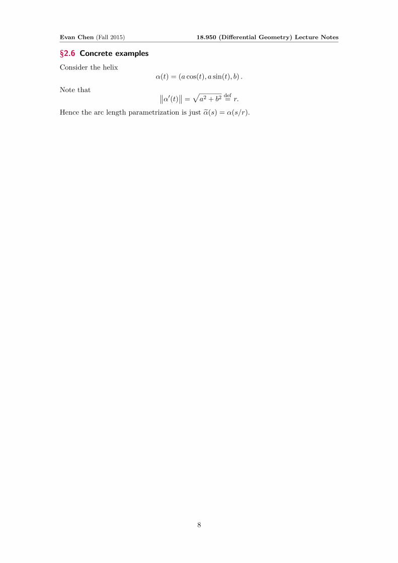
§2.6 Concrete examples

Consider the helixα(t) = (a cos(t), a sin(t), b) .

Note that ∥∥α′(t)∥∥ =√a2 + b2

def= r.

Hence the arc length parametrization is just α(s) = α(s/r).

8



§3.1 Always Cauchy-Schwarz

Pointing out explicitly from last lecture:

Proposition 3.1 (Triangle Inequality in the Spirit of L1)

For any f : I → Rn we have∥∥∥∥∫ `

0f(t) dt

∥∥∥∥ ≤ ∫ `

0‖f(t)‖ dt.

Proof. By components.

§3.2 Curvature

Assume we have a curve α : I → R3 with ‖α′(s)‖ = 1 meaning that α′(s) actuallyinterprets an angle. Then we can consider α′′(s), which measures the change in the angle.

Definition 3.2. The curvature k(s) is ‖α′′(s)‖.

Remark 3.3. Note that k(s) ≡ 0 if and only if α is a straight line.

Remark 3.4. The curvature remains unchanged by change of orientation.

Recall now that ‖α′(s)‖ = 1 ⇐⇒ α′′(s) ⊥ α′(s). Thus, we can define

n(s) =α′′(s)

‖α′′(s)‖.

and call this the normal vector. At this point we define t(s) as the tangent vectorα′(s). The plane spanned by α′(s) and α′′(s) is called the osculating plane.

Definition 3.5. If k(s) = 0 at some point we say s is a singular point of order 1.

§3.3 Torsion

Definition 3.6. The binormal vector b(s) is defined by t(s)× n(s).

Proposition 3.7

In R3 we have that b′(s) is parallel to n(s).

Proof. By expanding with Leibniz rule we can deduce

b′(s) = t(s)× n′(s).

Now, ‖b(s)‖ = 1 =⇒ b′(s) ⊥ b(s). Also, b′(s) ⊥ t(s). This is enough to imply theconclusion.

Definition 3.8. In light of this, we can define b′(s) = τ(s)n(s), and we call τ(s) thetorsion.

9


Proposition 3.9 (Plane Curve ⇐⇒ Zero Torsion)

The curve α is a plane curve only if it has zero torsion (meaning τ(s) ≡ 0 everywhere).

Proof. τ(s) = 0 ⇐⇒ b′(s) = 0 ⇐⇒ b(s) = b0 for a fixed vector b0. For one direction,note that if b(s) = b0 we have

d

ds[α(s) · b0] = α′(s) · b0 = t(s) · b0 = 0

the last step following from the fact that b(s) is defined to be normal to the tangentvector. Thus α(s) · b0 is constant, so we can take s0 such that

b0 · (α(s)− α(s0)) = 0

holds identically in s. The other direction is similar (take the derivative of the lpaneequation).

Remark 3.10. The binormal vector remains unchanged by change of orientation.

Example 3.11 (Helix)

Consider again the helix

α(s) =(a cos

s

r, a sin

s

r, bs

r

).

We leave to the reader to compute

b(s) =

(b

rsin(s/r),− b

rcos(s/r), a/r

).

Thus

b′(s) =

(b

r2cos(s/r),

b

r2sin(s/r), 0

).

One can also compute

n(s) =α′′(s)

k(s)= (− cos(s/r),− sin(s/r), 0) .

Thus one can obtain the torsion τ(s) = −b/r2.

§3.4 Frenet formulas

Let α : I → R3 be parametrized by arc length. So far, we’ve associated three orthogonalunit vectors

t(s) = α′(s)

n(s) =α′′(s)

‖α′′(s)‖b(s) = t(s)× n(s)

which induce a positive orientation of R3. We now relate them by:

10


Theorem 3.12 (Frenet Formulas)

We always have

t′(s) = k(s)n(s)

n′(s) = −k(s)t(s)− τ(s)b(s)

b′(s) = τ(s)n(s)

Proof. The first and third equation follow by definition. For the third, write n = b× tand differentiate both sides, applying the product rule.

So it seems like we can recover t, n, b from k, τ by solving differential equations. In fact,this is true:

Theorem 3.13 (Fundamental Theorem of the Local Theory of Curves)

Given differentiable functions k(s) > 0 and τ(s) on an interval I = (a, b), thereexists a regular parametrized curve α : I → R3 with that curvature and torsion.

Moreover, this curve is unique up to a rigid motion, in the sense that if α and αboth satisfy the condition, then there is an orthogonal linear map ρ : R3 → R3 withdet ρ > 0 such that α = p ◦ α+ c. Intuitively, this means “uniqueness up to rotationand translation”.

The uniqueness part is not difficult; the existence is an ordinary differential equation.

§3.5 Convenient Formulas

The curvature of an α not parametrized by arc length is

κ =|α′ × α′′||α′|3

.

The torsion is

τ = −(α′ × α′′) · α′′′

|α′ × α′′|2.

11



§4.1 Signed Curvature

We wish to describe signed curvature for a plane curve.Assume that α : I → R2, so we have a tangent vector t(s). Then we can give a unique

normal vector n(s) such that (t, n) forms a positive basis.

~t(s)

~n(s)

γ

Thus we can define the signed curvature according to

t′(s) = k(s)n(s)

which may now be either positive or negative.

§4.2 Evolute of a Curve

Given a plane curve α : I → R2, we define the evolute of α to be the curve

β(s) = α(s) +1

k(s)n(s).

Proposition 4.1 (Properties of the Evolute)

Let α(s) be a curve parametrized by arc length and β its evolute. Then

(a) β is normal to α, and

(b) Let s1 and s2 be points, and consider the intersection p of their normal vectorsto α. As s1, s2 → s, p→ β(s).

We call β(s) the center of curvature of α(s).

s1s2

γ

p

12


Proof. Part (a) is easy, since the Frenet equations imply n′(s) = −kt (as the torsionvanishes), and hence

β′(s) = α′(s)− 1

k(s)2k′(s)n(s) +

1

kn′(s) = t− k′

k2n+

1

k(−kt) = − k

′

k2n(s).

Part (b) involves more arithmetic. Let α(s) = (x(s), y(s)) so t(s) = (x′(s), y′(s)). Thenn(s) = (−y′(s), x′(s)). Now, given s1 and s2 we seek the point

p = α(s1) + λ1n(s1) = α(s2) + λ2n(s2)

for some λ1 and λ2. One can check after work that

λ1 =x′(s2)(x(s2)− x(s1)) + y′(s2)(y(s2)− y(s1))

y′(s2)x′(s1)− x′(s2)y′(s1).

In the limit, one can check that this becomes

lims1,s2→s

λ1 =x′(s)2 + y′(s)2

y′′(s)x′(s)− x′′(s)y′(s)=

1

y′′(s)x′(s)− x′′(s)y′(s)=

1

k(s).

Thus, α(s) + λ(s)n(s) = β(s) by definition.

§4.3 Isoperimetric Inequality

Problem 4.2. Of all simple closed curves in the plane with a given length `, which onebounds the largest area?

In this situation we have α : [a, b] → R3 a regular curve. It is closed if α(a) = α(b)and α(k)a = α(k)b for all k ∈ N. It is simple if it is not self-intersecting. We will quotewithout proof that

Theorem 4.3 (Jordan Curve Theorem)

A closed simple regular curve bounds a region in R2.

Thus one can assign the curve a positive orientation, namely the counterclockwise direction(formally, n(s) points into the bounded region D described by the Jordan curve theorem).

We will now give:

Theorem 4.4 (Isoperimetric Inequality)

Let α be a simple closed plane curve of length ` and let A be the area of the boundedregion. Then

`2 ≥ 4πA

with equality if and only if α gives a circle.

To bring areas into the picture, we also quote:

Theorem 4.5 (Special Case of Green’s Theorem)

Given closed simple regular α(t) = (x(t), y(t)) the area bounded is

A = −∫ b

ayx′ =

∫ b

axy′ =

1

2

∫ b

a(xy′ − yx′) dt

which can be found e.g. by using Green’s Theorem.

13


Proof of Isometric Inequality. Parametrize the original curve α = (x, y) by arc length.Thus α : [a, b]→ R2.

Suppose that x runs from a maximal right side coordinate xmax and a minimal xmin;we let 2r = xmax − xmin, and now draw a circle S with radius r, centered at the origin.Now we parametrize S by β but not by arc length: rather, we parametrize β so that thex-coordinates of β and α always coincide. So β : [a, b]→ S. Let β = (x, y).

Let A be the area of the bounded region. Then by our area form

A+ πr2 =

∫ b

a(xy′ − yx′) ds

≤∫ b

a

√(x2 + y2)(x′2 + y′2) ds

=

∫ b

a

√x2 + y2 ds

=

∫ b

ar ds

= `r

Now by AM-GM we have`r = A+ πr2 ≥ 2r

√Aπ

and this gives the desired bound on A.

14



We now begin the study of surfaces.

§5.1 Regular Surfaces

Definition 5.1. A regular surface is a subset S ⊆ R3 such that for every point p,there is a neighborhood p ∈ V ⊆ R3 which is diffeomorphic to an open subset of R2.

By diffeomorophic, we mean that there is a map

x : R2 ⊃ U → V ∩ S ⊂ R3

such that x is differentiable and bijective, with continuous inverse, and moreover the dif-ferential dx : R2 → R3 is injective (i.e. it has full rank). We call the x a parametrizationat x and the ordered triple (x, U, V ∩ S) a coordinate chart.

(We don’t yet require the inverse to be differentiable because at the moment our set Sonly has a topological structure, and don’t yet have a differential structure on S.)

In practice to check that the differential is injective one simply computes the associatedmatrix and evaluates the rank (say by finding a 2× 2 minor with full rank).

Example 5.2 (Projection of Sphere)

For a sphere S2 = {(x, y, z) | x2 + y2 + z2 = 1}, we can take a projection onto thexy, yz, zx planes for a total of six charts. For example on of the charts is

R2 ⊃ {u2 + v2 < 1} → R3 by (u, v) 7→ (u, v,√

1− u2 − v2).

Let’s verify this actually works. First, it is clear the map is differentiable. To seethat the differential has full rank, we simply use the first two coordinates and put

∂(u, v)

∂(u, v)= det

(1 00 1

)= 1.

Finally, we need to construct a continuous inverse. We just take the projection(x, y, z) 7→ (x, y). This is clearly continuous.

§5.2 Special Cases of Manifolds

As the above example shows it does take some time to verify the (rather long) definitionof a manifold. So we would like some way to characterize regular surfaces more rapidly.

One obvious way to do this is:

Theorem 5.3 (Graphs are Regular Surfaces)

Let U ⊂ R2 and f : U → R be differentiable. Then the graph of f , i.e. the set

{(x, y, f(x, y)) | (x, y) ∈ U}

is a regular surface.

Proof. Repeat the work we did when we checked the sphere formed a regular surface.Note that in this case we actually have a global parametrization, namely U → R3 by(x, y) 7→ (x, y, f(x, y)).

15


Here is a second way to do this. First, recall that

Definition 5.4. Given a differential map F : U → Rm (where U ⊂ Rn is open) a criticalpoint p ∈ U of F is one such that (dF )p : Rn → Rm is not surjective. The value of F (p)is called critical value.

Values in the image Rm which are not critical are called regular values.

In particular, if F : U → R then p is a critical value if and only if (DF )p vanishes, i.e.the gradient is zero.

Now we claim that

Theorem 5.5 (Level Images are Surfaces)

Let f : R3 ⊃ U → R is differentiable and c be a regular value. Then the pre-image{(x, y, z) ∈ R3 | f(x, y, z) = c

}is a regular surface.

The proof of this is essentially the inverse function theorem.

16


§6 September 29, 2015 and October 1, 2015

I was absent this week, so these notes may not be a faithful representation of the lecture.

§6.1 Local Parametrizations

Regular surfaces are nice because we have local coordinates at every point.

Proposition 6.1 (Local Parametrization as Graph)

Let S ⊂ R3 and p ∈ S. Then there exists a neighborhood V of p ∈ S such that Vis the graph of a differentiable function in one of the following forms: x = f(y, z),y = f(z, x), z = f(x, y).

Sketch of Proof. By definition of regular surface, we can take a parametrization at p.One of the Jacobian determinants is nonzero, by hypothesis.

Finally, we state a lemma that says that if we know S is regular already, and we havea candidate x for a parametrization x : U → R3 for U ⊂ R2, then we need not check x−1

is continuous if x is injective.

Proposition 6.2

Let p ∈ S for a regular surface S. Let x : U → R3 be differentiable with image inp such that the differential dx is injective everywhere. Assuming further that x isinjective then x−1 is continuous.

§6.2 Differentiability

We want a notion of differentiability for a function f : V → R where V is an open subsetof a surface S. This is the expected:

Definition 6.3. Let f : V ⊂ S → R be a function defined in an open subset V ofa regular surface S. Then f is differentiable at p ∈ V if for some parametrizationx : U ⊂ R2 → S, the composition

Ux−→ V

f−→ R.

is differentiable at x−1(p) (giving x−1(p) 7→ p 7→ f(p)).

One can quickly show this is independent of the choice of parametrization, so “forsome” can be replaced by “for all”.

§6.3 The Tangent Map

Given our embedding in to ambient space, we can define the tangent space as follows.

Definition 6.4. A tangent vector to p ∈ S is the tangent vector α′(0) of a smoothcurve α : (−ε, ε)→ S with α(0) = p.

The “type” of the “tangent vector” is actually vector in this case.

17


Proposition 6.5

Let x : U → S be a parametrization (U ⊂ R2). For q ∈ U , the vector subspace

dxq(R2) ⊂ R3

coincides with the set of tangent vectors of S at q.

In particular, dxq(R2) doesn’t depend on the parametrization x, so we denote it now byTp(S), the tangent space at S.

This lets us talk about the notion of a differential of a smooth map between surfaces.Specifically, suppose

S1 ⊃ Vφ−→ S2.

Then given a map α : (−ε, ε)→ V we get a composed path β

(−ε, ε)

V

α

?

φ- S

β

-

Proposition 6.6

Consider the situation above. The value of β′(0) depends only on α′(0), so we obtaina map

(dφ)p : Tp(S1)→ Tφp(S2).

Moreover, this map is linear; actually,

β′(0) = dφp(w) =

(∂φ1∂u

∂φ1∂v

∂φ2∂u

∂φ2∂v

)(u′(0)v′(0)

)where φ = (φ1, φ2) in local coordinates.

18


§7 October 6, 2015

§7.1 Local Diffeomorphism

Definition 7.1. A map φ : U ⊂ S1 → S2 is a local diffeomorphism at p ∈ U if thereexists a neighborhood p ∈ V ⊂ U such that φ is a diffeomorphism of V onto its image inS2.

Example 7.2 (Local 6= Global)

The map S1 → S2 by z 7→ z2 is a local diffeomorphism but not globally (since it isnot injective).

We can check whether functions are local diffeomorphisms by just their differen-tials.

Proposition 7.3 (Inverse Function Theorem)

Let S1 and S2 be regular surfaces, φ : U ⊂ S1 → S2 differentiable. If the differential

(dφ)p : TpS1 → Tφ(p)S2

is a linear isomorphism (full rank), then φ is a local diffeomorphism at p.

Proof. The point is that at p, φ(p), S1 and S2 look locally like Euclidean space. Usingthe parametrizations x and x respectively, we induce a map U → U whose differential isan isomorphism:

S1φ

- S2

U

x

?

6

- U

x

?

6

The classical inverse function theorem gives us an inverse map, which we then lift to amap of the surfaces.

§7.2 Normals to Surfaces

Let p ∈ S be a point, and let x : U → S be a local parametrization of S at p. Then wedefine the normal vector to the surface as follows: observe that the tangent space Tp(S)has a basis x1, x2 corresponding to the canonical orientation of R2 (as inherited by U).Then we define

N(p) = ± x1 × x2

|x1 × x2|.

Then, if two surfaces intersect at p, the angle between the surfaces is the angle betweenthe normal vectors.

§7.3 The First Fundamental Form

Let S ↪→ R3 be a regular surface. Then for any p ∈ S, the tangent plane TpS inherits aninner product from R3, because it is a subsace of R3.

19


Thus, we have a map

Ip : TpS → R by w 7→ 〈w,w〉 = ‖w‖2 .

Note that by abuse, we use 〈−,−〉 despite the fact that this form depends on p

Definition 7.4. The map Ip is called the first fundamental form of S at p ∈ S.

The power of Ip is that it lets us forget about the ambient space; we can talk aboutthe geometry of the surface by looking just at Ip. In fact, it was shown very recentlyby John Nash that the intrinsic and extrinsic notion of geometry coincide: roughly, anysuch surface with a fundamental form of this sort can be embedded in Rn.

To repeat: we will see that the first fundamental form allows us to makemeasurements on the surface without referring back to the ambient spaceR3.

One can compute this explicitly given local coordinates. Suppose we parametrizex : U ⊂ R2 → S and take p ∈ U . Then if we denote R2 = uR⊕ vR, then TpS has a basis{xu, xv}, where xu = ∂x

∂u(p) and xu = ∂x∂v (p).

Now, let w ∈ Tp(S). Let α : (−ε, ε)→ S such that α(t) = x(u(t), v(t)) and

w = α′(0) = u′(0)xu + v′(0)xv.

Then by expanding, we obtain

Ip(w) = 〈w,w〉p=⟨u′(0)xu + v′(0)xv, u

′(0)xu + v′(0)xv⟩

= ‖xu‖2 u′(0)2 + 2 〈xu, xv〉u′(0)v′(0) + ‖xv‖2 v′(0)2.

We write this as

= E · u′(0)2 + 2F · u′(0)v′(0) +G · v′(0)2.

where

E = 〈xu, xu〉F = 〈xu, xv〉G = 〈xu, xv〉 .

Example 7.5 (Plane)

Let P ⊂ R3 be the plane parametrized globally by a single chart

x(u, v) = p0 + uw1 + vw2

for some orthonormal vectors w! and w2. Then, (E,F,G) = (1, 0, 1).Then given any tangent vector w = aw1 + bw2 at an arbitrary point p we get

Ip(w) = a2 + b2; we just get the length of the vector.

20


Example 7.6 (Cylinder)

Consider the cylinderC =

{(x, y, z) | x2 + y2 = 1

}.

We now take the chartx(u, v) = (cosu, sinu, v)

where the domain is U = (0, 2π) × R; this covers most of the cylinder C (otherthan a straight line). We notice that the tangent plane is exhibited by the basisxu = (− sinu, cosu, 0) and xv = (0, 0, 1). Thus E = sin2 u + cos2 u = 1, F = 0,G = 1.

So the cylinder and the plane have the same first fundamental form. This is thegeometric manifestation of the fact that if we cut a cylinder along an edge, then weget a plane.

Example 7.7 (Stuff Depends on Parametrization)

Suppose now we use the parametrization on the cylinder

x(u, v) = (cosu, sinu, 5v)

Then the tangent plane is exhibited by the basis xu = (− sinu, cosu, 0) and xv =(0, 0, 5). Thus E = sin2 u+ cos2 u = 1, F = 0, G = 5.

§7.4 Relating curves by the first fundamental form

Let α : I → S be a regular curve. We already knew that the arc length is given by

s(t) =

∫ t

0

∥∥α′(t)∥∥ dt.If the curve is contained entirely within a chart α(t) = x(u(t), v(t)) then we may rewritethis as ∫ t

0

√Iα(t)α′(t) dt =

∫ t

0

√E(u′)2 + 2Fu′v′ +G(v′)2 dt.

Colloquially, we can write this as ds2 = E(du)2 + 2Fdudv +G(dv)2.Given α, β : I → S now with α(t0) = β(t0), the angle θ between the two tangent curves

is

cos θ =〈α′(t0), β′(t0)〉‖α′(t0)‖ ‖β′(t0)‖

. =

As a special case, suppose α and β are coordinate curves, meaning α′(t) = xu andβ′(t) = xv for all α, β. (Think rulings on a surface.) The angle between them xu and xvis thus given by

cosφ =〈xu, xv〉‖xu‖ ‖xv‖

=F√EG

.

Example application: loxodromes.

21


§7.5 Areas

Let R ⊂ S be a closed and bounded region of a regular surface contained in theneighborhood of a parametrization x : U ⊂ R2 → S. Let Q = x−1(R). The positivenumber ∫

Q‖xu × xv‖ du dv

does not depend on the choice of x and is defined as the area of R.In local coordinates, ‖xu × xv‖ =

√EG− F 2.

22


§8 October 8, 2015 and October 15, 2015

I am now attending roughly only every third class or so. Here are my notes from myown reading from the content I missed.

§8.1 Differentiable Field of Normal Unit Vectors

Let N : S → S2 ⊆ R3 be a map which gives a normal unit vector at each point.For example, if x : U → S (where U ⊂ R2) is a parametrization, then we define for

each q ∈ x(U) by

N(q) =xu × xv|xu × xv|

at q.

By abuse, we denote this Nq.More generally, if V ⊂ S is open, N : V → S2 ⊂ R3 is a differentiable map, then we

say that N is a differentiable field of normal unit vectors

Remark 8.1. Not all surfaces admit such a field of unit vectors (Mobius strip, forexample). Of course, most things (like spheres) do.

This N is called the Gauss map.

Example 8.2 (Cylinder)

Let S be the cylinder {(x, y, z) | x2 + y2 = 1}. We claim that N = (−x,−y, 0) areunit normal vectors. A tangent vector is given by α′(0) = (x′(0), y′(0), z′(0)) whereα = (x, y, z) has α(0) = p. Since x(t)2 + y(t)2, we see that along this curve, we seethat N · α′ = 0, as desired.

§8.2 Second Fundamental Form

In this way, N provides an orientation on S. We see in this case, for any point p we havea map

dNp : TpS → TN(p)S2 '−→ TpS

Example 8.3

Let S be the cylinder {(x, y, z) | x2 + y2 = 1}. Let us see what dNp does to tangentvectors. Using the setup with α as before (so α(0) = p), the tangent N(t) to α(t) is(−x(t),−y(t), z(t)) and thus

dNp

(x′(0), y′(0), z′(0)

)=(−x′(0),−y′(0), 0

).

In other words, dNp is projection onto the xy-plane. In particular, the tangents tothe cylinder parallel to the xy-plane are −1 eigenvectors while the tangents to thecylinder parallel to the z-axis are all mapped to zero (in the kernel).

Lemma 8.4 (dNp is self-adjoint)

As defined, dNp : TpS → TpS is self-adjoint, in the sense that

〈dNp(v), w〉 = 〈v, dNp(w)〉 .

23


Proof. Let α(0) = p, α(t) = x(u(t), v(t)), α′(0) = u′(0)xu + v′(0)xv. Write

dNp(α′(0)) =

[d

dt(N(u(t), v(t)))

]t=0

= Nuu′(0) +N ′vv

′(0).

So, it suffices to show that〈Nu, xv〉 = 〈xv, Nu〉 .

Take the derivatives of 〈N, xu〉 = 0 and 〈N, xv〉 = 0 relative to u and v to see that bothare equal to −〈N, xuv〉 = −〈N, xvu〉.

Definition 8.5. Let Ip be the quadratic form defined in Tp(S) by

Ip(v) = −〈dNp(v), v〉 = −〈v, dNp(v)〉 .

This is called the second fundamental form of S at p.

Now, let us think about curves for a moment.

Definition 8.6. Let C be a regular curve in S, and p ∈ S a point on it. Let k be thecurvature of C at p, and set cos θ = 〈n,N〉, where n is the normal to C and N is thenormal vector to S at p. The number kn = k cos θ is then called the normal curvatureof C ⊂ S at p.

In other words, kn is the length of the projection of the vector kn = α′ over the normalto the surface at p, with sign given by orientation.

Theorem 8.7 (Meusnier)

The normal curvature of a curve C at p depends only on the tangent line at thecurve.

Proof.

Thus, it make sense to talk about the curvature at a direction to the surface.

24


§9 October 20, 2015

§9.1 Self-Adjoint Maps

Since dNp is self-adjoint, there exists an orthonormal basis {e1, e2} of TpS such that

dNp(e1) = −k1e1 and dNp(e2) = −k2e2.

Definition 9.1. The constant k1 and k2 are called the principal curvature and thebasis e1 and e2 are called the principal directions.

Given w ∈ TpS, say w = cos θe1 + sin θe2, then the value of the normal curvature tokn along w is

−〈dNp(cos θe1 + sin θe2), cos θe1 + sin θe2〉 = 〈k1 cos θe1 + k2 sin θe2, cos θe1 + sin θe2〉= k1 cos2 θ + k2 sin2 θ.

So we can express any normal curvature in terms of the principal ones.

§9.2 Line of Curvatures

Definition 9.2. If a regular curve C on S has the property that for all p ∈ C, thetangent line of C at p is a principal direction at p, then C is called a line of curvatureof S.

Example 9.3 (Examples of Lines of Curvatures)

(a) In a plane, all curves are lines of curvature (trivially). (dNp = 0, so everythingis an eigenvalue.)

(b) All curves on a sphere are also lines of curvature. (dNp = id, so everything isan eigenvalue.)

(c) On a cylinder, the vertical lines and the meridians are lines of curvatures of S.

Proposition 9.4 (Testing for Line of Curvature)

Let C be a regular curve. Then C is a line of curvature if and only if

dNp(α′(t)) = λ(t)α′(t)

where α(t) is the arc length parametrization, and λ(t) ∈ R.

Proof. “Harmless exercise”. (A better word might be “trivial”.)

§9.3 Gauss curvature and Mean Curvature

In the orthonormal basis of p, we have dNp = −(k1 00 k2

). Of course, we define

Definition 9.5. The quantity det dNp = k1k2 is called the Gauss curvature. Thequantity Tr(dNp) = −(k1 + k2) is more finicky. We instead define H = 1

2(k1 + k2) =−1

2 Tr(dNp) the mean curvature.

25


Remark 9.6. One can view H as the “average” of all curvatures of curves passingthrough H.

Definition 9.7. A point p ∈ S is called

• elliptic if det(dNp) > 0, meaning k1 and k2 have the same sign.

• hyperbolic if det(dNp) < 0,

• parabolic if det(dNp) = 0, but dNp 6= 0, and

• planar if dNp is the zero matrix.

It’s worth noting that planes are not the only example where planar points. For example,if z = x4, and we wrote this around the z-axis to get a surface (i.e. z = (x2 + y2)2) thenthe origin is also a planar point.

Definition 9.8. An umbilical point of S is a point p ∈ S at which k1 = k2, meaningdNp is a constant times the identity.

Theorem 9.9

All connected surfaces S which consist entirely of umbilical points are subsets of thesphere or a plane.

Proof. Prove it locally first. Then for any fixed p, for other q ∈ S take a path from p toq, and use compactness.

§9.4 Gauss Map under Local Coordinates

Let p ∈ S where S is an regular surface with an orientation N : S → S2 ⊂ R3. For p ∈ Sand x : U → S a parametrization near p, we can set

α(t) = x(u(t), v(t)) ∈ S

such that α(0) = p. So,α′ = u′xu + v′xv

where xu and xv are the usual basis of TpS (i.e. the partial derivatives of x with respectto u and v). Thus, it follows that

dNp(α′) =

d

dtN(u(t), v(t)) = u′Nu + v′Nv.

So, we simply need to compute Nu and Nv. If we sidestep this for now and sayNu = a11xu + a21xv, and Nv = a12xu + a22xv, then this reads

dNp

(u′

v′

)=

(a11u

′ + a12v′

a21u′ + a22v

′

)=

(a11 a12

a21 a22

)(u′

v′

).

Note that the matrix

(a11 a12

a21 a22

)need not be symmetric unless xu and xv are orthogonal.

(Self-adjoint implies symmetric only in this case.)One can compute the aij , but since I really don’t want to. The result is called the

equations of Weingarten.

26


§10 October 22, 2015

§10.1 Completing Equations of Weingarten

Let me finish the computation from last time. Take α(t) = x(u(t), v(t)), α(0) = p, Recallthe we have written

Nu = a11xu + a21xv

Nv = a11xu + a21xv

(again these subscripts are partial derivatives at the point p). The point is that

dNp : TpS → TpS by u′xu + v′xv 7→ u′Nu + v′Nv

where Nu, Nv ∈ TpS as well. Thus, We have that

Ip(α′) =⟨Nuu

′ +Nvv′, xuu

′ + xvv′⟩ def

= e(u′)2 + 2fu′v′ + g(v′)2

for e = −〈Nu, xu〉 = 〈N, xuu〉 and similarly for others. If we use the first equation, thenputting in the aij we derive

−(e ff g

)=

(a11 a12

a21 a22

)︸︷︷︸

dNp

(E FF G

).

In particular, we have

k1k2 = det dNp =eg − f2

EG− F 2.

Through pain and suffering, we also can compute

H =1

2(k1 + k2) =

1

2

eG− 2fF + gE

EG− F 2.

§10.2 An Example Calculation

We consider a torus, parametrized by

x(u, v) = ((a+ r cosu) cos v, (a+ r cosu) sin v, r sinu) .

The partial derivatives are

xu = (−r sinu cos v,−r sinu sin v, r cosu)

xv = (−(a+ r cosu) sin v, (a+ r cosu) cos v, 0) .

Thus, we can extract

E = 〈x,xu〉 = r2

F = 〈xu, xv〉 = 0

G = 〈xv, xv〉 = (a+ r cosu)2.

27


Let N = xu×xv|xu×xv | , noting that the denominator is

√EG− F 2. We define the constants

e = 〈Nu, xu〉= 〈N, xuu〉

=

det

−r sinu cos v −r sinu sin v r cosu−(a+ r cosu) sin v (a+ r cosu) cos v 0−r cosu cos v −r cosu sin v −r sinu

√EG− F 2

=r2(a+ r cosu)

r(a+ r cosu)= r.

Similarly,

f = 〈N, xuv〉 = · · · = 0

g = 〈N, xvv〉 = · · · = cosu(a+ r cosu).

Thus, we have

K =cosu

r(a+ r cosu).

§10.3 Elliptic and Hyperbolic Points

Proposition 10.1

Let p ∈ S with S a regular surface.

• If p ∈ S is elliptic, then all points in some neighborhood of S are on one sideof the tangent plane TpS

• If p ∈ S is hyperbolic, for any neighborhood of p there is a point on both sidesof TpS.

Proof. Let x(u, v) be a parametrization near p, with x(0, 0) = p. We’re interested in thesigns of the function

f(u, v) = 〈x(u, v)− x(0, 0), N〉

with Np the normal at p. Locally, we have

x(u, v) = x(0, 0) + xu(0, 0)u+ xv(0, 0)v +1

2

[xuuu

2 + 2xuvuv + xvvv2]

+R

with R an error term with Ru2+v2

→ 0 as (u, v)→ 0. Now, 〈xu(0, 0), N〉 = 〈xv(0, 0), N〉 =

0. If we expand and go through the computation, denoting R = 〈R,N〉 one can compute

f(u, v) =1

2Ip(uxu + vxv) +R =

u2 + v2

2

(Ip(

(u, v)√u2 + v2

)+

R

u2 + v2

).

Suppose first that k1 ≥ k2 > 0. Then Ip(

(u,v)√u2+v2

)= 1

2(k1 cos2 θ + k2 sin2 θ) ≥12 min{k1, k2} is bounded away from zero. So for u2 + v2 small enough, f(u, v) ≥ 0.An analogous argument works if k1 > 0 > k2.

28


§10.4 Principal Directions

Theorem 10.2 (Criteria for Principal Directions)

Fix a point p ∈ S. Then u′xu + v′xv is an eigenvector of (dN)p if and only if

0 = det

(v′)2 −u′v′ (u′)2

E F Ge f g

.

29


§11 October 29, 2015 and November 3, 2015

§11.1 Isometries

Let S1 and S2 be surfaces.

Definition 11.1. A diffeomorphism φ : S → S′ is an isometry if for all w1 and w2 inTp(S), we have

〈w1, w2〉p = 〈(dφ)p(w1), (dφ)p(w2)〉φ(p) .

In that case, we say S1 and S2 are isometric.

Naturally, this means that the first fundamental form Ip is preserved. In fact, byconsidering 〈v + w, v + w〉 − 〈v, v〉 − 〈w,w〉 we see that isometries are equivalent topreserving just the first fundamental form.

Definition 11.2. Let p ∈ V ⊂ S′, where S′ is a surface. A map φ : V → S, where Vis a neighborhood of some surface, is a local isometry at p if it is an isometry onto aneighborhood of φ(p)

We say S locally isometric to S′ if one can find a local isometry into S′ at everypoint p ∈ S. If the other direction holds too, we say the surfaces are locally isometric.

Properties that are preserved under local isometry are said to be intrinsic. for example,the first fundamental form is intrinsic.

Example 11.3 (Cylinder and Plane are Locally Isometric)

The cylinder is locally isometric to a plane (0, 2π)× R, but not globally (since thespaces are not homeomorphic, their fundamental groups differ).

Example 11.4 (Half-Cylinder and Plane are Globally Isometric)

Half a cylinder is globally isometric to the plane (0, π)× R. Note that the secondfundamental form of a cylinder is nonzero (unlike the plane),

Thus, second fundamental form is not intrinsic. In fact, we will later see that the meancurvature is not intrinsic, but the global curvature is.

For aid with local coordinates:

Proposition 11.5

Suppose x : U → S and x′ : U → S′ are parametrizations such that we have anequality E = E′, F = F ′ and G = G′ of the coefficients of the first fundamentalform. Then x′ ◦ x−1 is a local isometry.

§11.2 The Christoffel Symbols

This is some very long calculations. The idea is that xu, xv, N form a triple of orthogonalvectors at every point p of the surface. Then, we can let

xuu = Γ111xu + Γ2

11xv + eN

xuv = Γ112xu + Γ2

12xv + fN

xvu = Γ121xu + Γ2

21xv + fN

xvv = Γ122xu + Γ2

22xv + gN.

30


Here the e, f , g coefficients were realized by taking the inner form of each equationwith N . Also, note that xuv = xvu, so Γi12 = Γi21 for i = 1, 2. We say the Γijk are theChristoffel symbols.

§11.3 Gauss Equations and Mainardi-Codazzi

If we take dot products of all relations with xu and xv, we obtain a system of equationsthat lets us solve for everything in terms of E, F , G and their derivatives with respect tou, v. (Note e, f , g are not present!)

There are some more relations we can derive. For example, note that

(xuu)v = (xuv)u.

It turns out that by expanding this and equating the xu coefficients, we obtain that

−KE = (Γ212)u − (Γ2

11)v + Γ112Γ2

11 + Γ212Γ2

12 − Γ211Γ2

22 − Γ111Γ2

12

where K is the Gauss curvature; this is the Gauss equation (Equating the xv coefficientsturns out to give the same equation.) The philosophical point is that it implies:

Theorem 11.6 (Theorema Egregium, due to Gauss)

The Gaussian curvature K is intrinsic, i.e. it is invariant under local isometries.

On the other hand, equating the N coefficients gives

ev − fu = eΓ112 + f(Γ2

12 − Γ111)− gΓ2

11.

Doing a similar thing gives

fv − gu = eΓ122 + f(Γ2

22 − Γ112)− gΓ2

12.

These two relations are called the Mainardi-Codazzi equations.

§11.4 Bonnet Theorem

We may wonder if we can get more relations. The answer is no.

Theorem 11.7 (Bonnet)

Let E, F , G, e, f , g be differentiable functions V → R, with V ⊂ R2. AssumeE,G > 0, that Gauss and Codazzi holds, and moreover EG− F 2 > 0. Then:

(a) for every q ∈ V there is a neighborhood U of V such that a diffeomorphismx : U → R3 such that x(U) is a surface having the above coefficients.

(b) this x is unique up to translation and orthogonal rotation.

31


§12 November 5, 10, 12, 17, 19 2015

In what follows, a vector field w on a surface S will mean a differentiable vector field oftangents; i.e. w(p) ∈ TpS for every p ∈ S.

§12.1 The Covariant Derivative

Definition 12.1. Let w be a vector field, and let y ∈ TpS be a tangent vector, realized byy = α′(0) for α : (−ε, ε)→ S parametrized. The covariant derivative is the projectionof (w ◦ α)′(0) onto the tangent plane, and denoted (Dyw)(p). We also denoted it by(Dw/dt)(0) if α is given.

This of course does not depend on α. We can apply an analogous definition if w isonly defined along points of a given path α.

In particular, this is zero if and only if (w ◦α)′ is parallel to the normal vector of Tp(S).One standard example is the case w = α′.

§12.2 Parallel Transports

Definition 12.2. Let α be a parametrized curve and w a vector field defined on it. Wesay α is parallel if Dw/dt is zero everywhere on α.

In other words, this occurs if for every α(t) = p and y = α′(t) we have (Dyw)(p) isparallel to the normal vector of Tp(S). In particular if S is the plane this is equivalent tow being constant.

Proposition 12.3

Let w and v be parallel vector fields along α. Then 〈w(t), v(t)〉 is fixed.

Thus parallel vector fields preserve angles and have constant lengths.By theory of differential equations, we have

Theorem 12.4 (Unique Parallel Vector Field)

Let α be a parametrized curve in S and pick a fixed initial vector w0 ∈ Tα(0)S. Thenthere exists a unique parallel vector field w along α such that w(0) = w0.

So in this way we can define the parallel transport along a parametrized curve: givenα joining p to q, for any vector w ∈ Tp(S) we can follow along the parallel vector field qto get a unique tangent vector in Tq(S).

§12.3 Geodesics

Most important special case of parallelism:

Definition 12.5. If α(s) is a regular parametrized curve and α′ is parallel, then α issaid to be a geodesic.

In this case, it means that the normal vectors ~n for α coincide with normal vectors tothe surface itself.

32


Theorem 12.6 (Unique Geodesic in Any Direction)

Let p be a point of a regular surface S and 0 6= w ∈ Tp(S). There is a geodesicα : (−ε, ε) → S with α(0) = p, and α′(0) = w, with the usual uniqueness up todomain.

Example 12.7 (Examples of Geodesics)

(a) Straight lines are always geodesics, because their normal vector vanishesaltogether.

(b) In particular, on a plane, the straight lines are the only geodesics.

(c) On a sphere, the great circles are the unique geodesics.

(d) On a right cylinder, geodesics are helixes.

More generally, let α be a regular parametrized curve on an oriented surface S. At apoint p, consider the tangent vector α′ = ~t and then the vector α′′. We can project itonto the Tp(S) as before, arriving at Dα′/ds; its signed length (with respect to N ×~t) isthe geodesic curvature kg. Thus geodesics are those curves with kg = 0.

Remark 12.8. Since kn is the other projection, k2 = k2n + k2

g .

33


§13 November 24 and 26, 2015

The main point of this section is to present the Gauss-Bonnet Theorem.

§13.1 Area Differential Form

This is technically review, but anyways. Let x : U → R3 be a parametrization. We canperform integrals of the form∫

Rf(u, v) |xu ∧ xv| =

∫x−1(R)

f(u, v)√EG− F 2 du ∧ dv

which is the integral of f over the region U . This is the pullback of the differential formxu ∧ xv on the surface. For convenience, we will abbreviate this to∫

Rf dσ.

§13.2 Global Gauss-Bonnet Theorem

We then have the following.

Theorem 13.1 (Gauss-Bonnet)

Let R ⊂ S be a regular region of an oriented surface S and let C1, . . . , Cn bepositively oriented curves forming the boundary of R. Let θ1, . . . , θp be the p =

(n2

)external angles formed by the Ci. Then

n∑i=1

∫Ci

kg(s) ds+

∫RK dσ +

p∑i=1

θi = 2πχ(R)

where χ is the Euler characteristic.

Corollaries:

Corollary 13.2 (Gauss-Bonnet for Simple Regions)

If R is a simple region, then χ(R) = 1 and thus

n∑i=1

∫Ci

kg(s) ds+

∫RK dσ +

p∑i=1

θi = 2π.

Corollary 13.3 (Gauss-Bonnet for Orientable Compact Surfaces)

If S is a orientable compact surface then∫SK dσ = 2πχ(S).

Proof. Take R = S, and use an empty boundary.

34


§14 December 1 and December 3, 2015

§14.1 The Exponential Map

Let S be a regular surface and p ∈ S a point. We consider the tangent plane Tp(S). Fora vector v ∈ Tp(S), we can consider the geodesic γv with γ′v(0) = v. In the event thatγ(1) is defined, we define the exponential map by

expp(v) = γv(1)

and set expp(0) = p.

Example 14.1 (Examples of the Exponential Map)

Let S = S2 be a sphere, and p ∈ S.

(a) expp(v) is defined for each v ∈ Tp(S). If |v| = (2k + 1)π, then expp(v) = −p,while if |v| = 2kπ then expp(v) = p.

(b) If we delete −p from S then expp is only defined in an open disk of radius π.

Proposition 14.2 (expp Defined Locally)

There exists a neigborhood U of 0 ∈ Tp(S) such that expp is defined, meaning wehave a map

expp : U → S,

and moreover expp is a diffeomorphism.

We say that V ⊂ S is a normal neighborhood of p if V is the diffeomorphic imageunder expp of some neighborhood U of Tp(S).

§14.2 Local Coordinates

We can impose coordinates on normal neighborhoods of a point via the exponential map,since it’s a diffeomorphism.

If we put rectangular coordinates (u, v), then the geodesics of S correspond to straightlines through the origin.

Now consider a polar coordinate system with 0 < θ < 2π and radius ρ, so pairs (ρ, θ).Note this omits the half-line ` corresponding to θ = 0. The images of circles at U(centered at zero) in S are then called the geodesic circles of V while the images of linesthrough 0 are called the radial geodesics; these correspond to setting ρ and θ constant.

Theorem 14.3 (First Fundamental Form in Geodesic Polar Coordinates)

Let x : U \ ` → V \ L be a system of geodesic polar coordinates (ρ, θ). Then thefirst fundamental form obeys

E = 1, F = 0, G(ρ, θ) = ρ− K(p)

6ρ3 + o(ρ3).

The fact that F = 0 reflects the so-called Gauss lemma: radial geodesics are orthogonalto the geodesic circles.

35


§15 December 8 and December 10, 2015

Our goal is to prove the Bonnet Theorem:

Theorem 15.1 (Bonnet’s Theorme)

Let S be a complete surface. Suppose there exists a δ > 0 such that the Gaussiancurvature K is bounded below by δ. Then S is compact and any two points arejoined by a geodesic with length at most π√

δ.

This is “optimal” by taking a sphere. (Definition of “complete” in next section.)

§15.1 Completeness

Definition 15.2. A regular connected surface S is complete if for any point p ∈ S theexponential map expp : Tp(S)→ S is defined for every v ∈ Tp(S).

Theorem 15.3 (Complete Surfaces are Nonextendible)

A complete surface S is nonextendible, i.e. it is not a proper subset of any regularconnected surface.

Theorem 15.4 (Closed Surfaces Are Complete)

Any closed surface S ⊆ R3 is complete. In particular, any compact surface iscomplete.

Complete surfaces have a nice notion of “distance”.

Theorem 15.5 (Hopf-Rinow)

If S is a complete surface then for any p, q ∈ S there is a minimal geodesic joining pto q.

Thus we may define the distance between two points on a complete surface by consideringthe minimal geodesic.

§15.2 Variations

In what follows, S is regular and connected but not necessarily complete.To do this, consider a curve γ : [0, `]→ S parametrized by arc length. A variation of

γ is a differentiable maph : [0, `]× (−ε, ε)→ S.

such that h(s, 0) = γ(s) for each s. We assume also that our variation h is proper,meaning h(0, t) = γ(0) and h(`, t) = γ(1). (In other words, h is a path homotopy.)

This then gives rise to a vector field

V (s) =

[∂

∂th(s, t)

]t=0

.

36


which we call the variational vector field of h. Since h is proper it follows thatV (0) = V (`) = 0.

Define L : (−ε, ε)→ R by letting L(t) be the arc length of h(−, t). Formally,

L(t) =

∫ `

9

∥∥∥∥∂h∂s (s, t)

∥∥∥∥ ds.Thus L(t) measures the arc length of the “nearby” curves specified by the variation h.

Theorem 15.6 (The First Variation)

We have

L′(0) = −∫ `

0〈A(s), V (s)〉 ds

where

A(s) =D

∂s

[∂h

∂s(s, 0)

].

Proof. Some direct computation. You need the fact that V (`) = V (0) = 0.

Remark 15.7. The vector A(s) is the acceleration vector of α and ‖A(S)‖ is thegeodesic curvature of α.

Now we can formally write down that geodesics are “locally minimal”.

Theorem 15.8 (Geodesics Are Minimal For Any Variation)

Given α : [0, `]→ S parametrized by arc length we have α is a geodesic if and onlyif for any proper variation h of α, we have L′(0) = 0.

Proof. If α is a geodesic, then A(s) ≡ 0 and the result is immediate.Otherwise, support V (s) = f(s)A(s) for some nonnegative “weight” function f sup-

ported on (0, `) where f(0) = f(`) = 0. By differential equations, we can construct hwith this variation. Now according to the previous result,

L′(0) = −∫ `

0〈A(s), A(s)f(s)〉 ds = −

∫ `

0f(s) ‖A(s)‖2 ds ≤ 0

which can only be zero if A(s) ≡ 0.

§15.3 The Second Variation

From now on, assume γ : [0, `]→ S is arc length, V (s) is proper, and V (0) = V (`) = 0,and moreover that we have an orthogonality relation⟨

V (s), γ′(s)⟩

= 0.

In other words we assume V is an orthogonal variation.We aim to compute L′′(0).

37


Lemma 15.9 (Partials Don’t Commute)

Let x : U → S be a parametrization at p ∈ S. Let K be the Gaussian curvature atp. Then

D

∂v

D

∂uxu −

D

∂u

D

∂vxu = K(xu × xv)× xu.

Proof. More direct computation with Christoffel symbols.

Remark 15.10. Philosophically, “curvature is something you can see by changing theorders of derivatives”.

Lemma 15.11

Let h : [0, `]× (−ε, ε) → S, and let W (s, t) = ∂h∂t (s, t) be a differential vector field

along h. Then we have

D

∂t

D

∂sW − D

∂s

D

∂tW = K(s, t)

(∂h

∂s× ∂h

∂t

)×W.

Theorem 15.12 (The Second Variation)

Suppose γ is a geodesic parametrized by arc length, and h : [0, `]× (−ε, ε)→ S be aproper orthogonal variation of of γ. Letting V be its variational vector field,

L′′(0) =

∫ `

0

(∥∥∥∥D∂sV (s)

∥∥∥∥2

−K(s) ‖V (s)‖2)ds

where K(s) is the Gaussian curvature at h(s, 0) = γ(s).

Proof. We take the derivative of the formula

L′(t) =

∫ `

0

⟨D∂s

∂h∂t (s, t),

∂h∂s (s, t)

⟩⟨∂h∂s (s, t), ∂h∂s (s, t),

⟩ 12

that we previously obtained. Move the differential operator through the integral sign.This gives us, by repeatedly applying Product Rule,

L′′(0) =

∫ `

0

[⟨D

∂t

D

∂s

∂h

∂t(s, 0),

∂h

∂s(s, 0)

⟩+

∥∥∥∥D∂sV (s)

∥∥∥∥2

−⟨D

∂sV (s),

∂h

∂s(s, 0)

⟩]ds.

Do some further computation now.

§15.4 Proof of Bonnet Theorem

Now that we have L′(0) and L′′(0) we can prove Bonnet’s Theorem.Assume S is complete, and K ≥ δ at all points of S. Consider two points p and q such

that the distance p, q is maximized, and let γ : [0, `]→ S be the minimal geodesic whichjoins them (permissible by the Hopf-Rinow Theorem). Now assume for contradiction` > π√

δThus we have L′(0) = 0. But if we can show L′′(0) < 0, then we will have shown

38


γ is in fact a local maximum and this will be a contradiction. (To see this: imagine thelong geodesic joining two points on a sphere. While locally the shortest path, globally itis longer than any perturbation.)

Consider proper variations V ; we have

L′′(0) =

∫ `

0

[∥∥∥∥D∂sV (s)

∥∥∥∥2

−K(s) ‖V (s)‖2]ds.

Pick a tangent vector w0 ∈ Tp(S) such that w0 ⊥ γ′(0) and ‖w0‖ = 1, and let w(t) be aparallel transport of w0 along γ. Then we define V (s) again by

V (s) = sin(π`s)w(s).

As V (0) = V (`) = 0, we again can construct an h corresponding to it. Then directcalculation gives

D

∂sV (s) = −π

`cos(

π

`s)w(s) + sin(

π

`s)D

∂sw(s)︸︷︷︸

=0∥∥∥∥D∂sV (s)

∥∥∥∥2

=π2

`2cos2(

π

`s)

‖V (s)‖2 = sin2(π

`s).

If K ≥ δ > π2

`2, then we have

L′′(0) < −π2

`2

∫ `

0

(cos2(

π

`s)− sin2

(π`s))

ds < −π2

`2

∫ `

0

(cos(2

π

`s))ds = 0

which is the desired contradiction.The choice of sin is designed for the ending. If we had used an arbitrary function f as

before, we would have 〈f ′′(s) + k(s)f(s), f(s)〉. So we choose a function f for which thisbecomes a zero integral.

39


§A Examples

Here is a collection of facts about some common examples. Recall for convenience that

K = EG− F 2 and H =1

2

eG− 2Ff + gE

EG− F 2.

§A.1 Sphere

Parametrize the unit sphere S2 in R3 by x(u, v) = (R cosu cos v,R cosu cos v,R sin v).

E = R2, F = 0, G = (R cosu)2

e = R, f = 0, g = R cos2 u.

The Gauss curvature at all points is the constant K = 1R2 . The mean curvature for this

parametrization is H = 1R . The geodesics are the great circles.

The genus of S2 is zero, so its Euler characteristic is 2. This surface is a compactoriented manifold without boundary.

§A.2 Torus

Parametrize a torus by x(u, v) = ((a+ r cosu cos v), (a+ r cosu sin v), r sinu).

E = r2, F = 0, G = (a+ r cosu)2

e = r, f = 0, g = cosu(a+ r cosu).

The Gauss curvature isK =

cosu

r(a+ r cosu).

The mean curvature is

H =a+ 2r cosu

2r(a+ r cosu).

The genus of S1 × S1 is 1, so its Euler characteristic is 0. This surface is a compactoriented manifold without boundary.

§A.3 Cylinder

Parametrize the cylinder by x(u, v) = (R cosu,R sinu, v). Then

E = R2, F = 0, G = 1.

e = −R, f = 0, g = 0.

The Gauss curvature is K = 0 everywhere. The mean curvature at all points is − 1R . The

geodesics are helixes, including meridians and vertical lines.This surface is not compact, but it is orientable, with empty boundary. It has genus 1

and Euler characteristic zero.

40

Documents

18.950 (Di erential Geometry) Lecture Notes · 2018-05-09 · Evan Chen (Fall 2015) 18.950 (Di erential Geometry) Lecture Notes §1September 10, 2015 Here is an intuitive sketch of