19. BIG-BANG COSMOLOGY

19. Big-Bang cosmology 1

19. BIG-BANG COSMOLOGYRevised September 2009 by K.A. Olive (University of Minnesota) and J.A. Peacock(University of Edinburgh).

19.1. Introduction to Standard Big-Bang Model

The observed expansion of the Universe [1,2,3] is a natural (almost inevitable) result ofany homogeneous and isotropic cosmological model based on general relativity. However,by itself, the Hubble expansion does not provide sufficient evidence for what we generallyrefer to as the Big-Bang model of cosmology. While general relativity is in principlecapable of describing the cosmology of any given distribution of matter, it is extremelyfortunate that our Universe appears to be homogeneous and isotropic on large scales.Together, homogeneity and isotropy allow us to extend the Copernican Principle to theCosmological Principle, stating that all spatial positions in the Universe are essentiallyequivalent.

The formulation of the Big-Bang model began in the 1940s with the work of GeorgeGamow and his collaborators, Alpher and Herman. In order to account for the possibilitythat the abundances of the elements had a cosmological origin, they proposed thatthe early Universe which was once very hot and dense (enough so as to allow for thenucleosynthetic processing of hydrogen), and has expanded and cooled to its presentstate [4,5]. In 1948, Alpher and Herman predicted that a direct consequence of thismodel is the presence of a relic background radiation with a temperature of order a fewK [6,7]. Of course this radiation was observed 16 years later as the microwave backgroundradiation [8]. Indeed, it was the observation of the 3 K background radiation that singledout the Big-Bang model as the prime candidate to describe our Universe. Subsequentwork on Big-Bang nucleosynthesis further confirmed the necessity of our hot and densepast. (See the review on BBN—Sec. 20 of this Review for a detailed discussion of BBN.)These relativistic cosmological models face severe problems with their initial conditions,to which the best modern solution is inflationary cosmology, discussed in Sec. 19.3.5. Ifcorrect, these ideas would strictly render the term ‘Big Bang’ redundant, since it wasfirst coined by Hoyle to represent a criticism of the lack of understanding of the initialconditions.

19.1.1. The Robertson-Walker Universe :The observed homogeneity and isotropy enable us to describe the overall geometry

and evolution of the Universe in terms of two cosmological parameters accounting forthe spatial curvature and the overall expansion (or contraction) of the Universe. Thesetwo quantities appear in the most general expression for a space-time metric which has a(3D) maximally symmetric subspace of a 4D space-time, known as the Robertson-Walkermetric:

ds2 = dt2 − R2(t)[

dr2

1 − kr2+ r2 (dθ2 + sin2 θ dφ2)

]. (19.1)

Note that we adopt c = 1 throughout. By rescaling the radial coordinate, we can choosethe curvature constant k to take only the discrete values +1, −1, or 0 correspondingto closed, open, or spatially flat geometries. In this case, it is often more convenient

C. Amsler et al., PL B667, 1 (2008) and 2009 partial update for the 2010 edition (http://pdg.lbl.gov)January 28, 2010 12:02

2 19. Big-Bang cosmology

to re-express the metric as

ds2 = dt2 − R2(t)[dχ2 + S2

k(χ) (dθ2 + sin2 θ dφ2)]

, (19.2)

where the function Sk(χ) is (sin χ, χ, sinh χ) for k = (+1, 0,−1). The coordinate r (inEq. (19.1)) and the ‘angle’ χ (in Eq. (19.2)) are both dimensionless; the dimensions arecarried by R(t), which is the cosmological scale factor which determines proper distancesin terms of the comoving coordinates. A common alternative is to define a dimensionlessscale factor, a(t) = R(t)/R0, where R0 ≡ R(t0) is R at the present epoch. It is alsosometimes convenient to define a dimensionless or conformal time coordinate, η, bydη = dt/R(t). Along constant spatial sections, the proper time is defined by the timecoordinate, t. Similarly, for dt = dθ = dφ = 0, the proper distance is given by R(t)χ. Forstandard texts on cosmological models see e.g., Refs. [9–16].

19.1.2. The redshift :The cosmological redshift is a direct consequence of the Hubble expansion, determined

by R(t). A local observer detecting light from a distant emitter sees a redshift infrequency. We can define the redshift as

z ≡ ν1 − ν2

ν2 v12

c, (19.3)

where ν1 is the frequency of the emitted light, ν2 is the observed frequency and v12

is the relative velocity between the emitter and the observer. While the definition,z = (ν1 − ν2)/ν2 is valid on all distance scales, relating the redshift to the relative velocityin this simple way is only true on small scales (i.e., less than cosmological scales) suchthat the expansion velocity is non-relativistic. For light signals, we can use the metricgiven by Eq. (19.1) and ds2 = 0 to write

v12

c= R δr =

R

Rδt =

δR

R=

R2 − R1

R1, (19.4)

where δr(δt) is the radial coordinate (temporal) separation between the emitter andobserver. Thus, we obtain the simple relation between the redshift and the scale factor

1 + z =ν1

ν2=

R2

R1. (19.5)

This result does not depend on the non-relativistic approximation.

January 28, 2010 12:02


19.1.3. The Friedmann-Lemaıtre equations of motion :The cosmological equations of motion are derived from Einstein’s equations

Rµν − 12gµνR = 8πGNTµν + Λgµν . (19.6)

Gliner [17] and Zeldovich [18] have pioneered the modern view, in which the Λ termis taken to the rhs and interpreted as an effective energy–momentum tensor Tµν for thevacuum of Λgµν/8πGN. It is common to assume that the matter content of the Universeis a perfect fluid, for which

Tµν = −pgµν + (p + ρ)uµuν , (19.7)

where gµν is the space-time metric described by Eq. (19.1), p is the isotropic pressure, ρis the energy density and u = (1, 0, 0, 0) is the velocity vector for the isotropic fluid inco-moving coordinates. With the perfect fluid source, Einstein’s equations lead to theFriedmann-Lemaıtre equations

H2 ≡(

R

R

)2

=8π GN ρ

3− k

R2+

Λ3

, (19.8)

andR

R=

Λ3− 4πGN

3(ρ + 3p) , (19.9)

where H(t) is the Hubble parameter and Λ is the cosmological constant. The first of theseis sometimes called the Friedmann equation. Energy conservation via T

µν;µ = 0, leads to a

third useful equation [which can also be derived from Eq. (19.8) and Eq. (19.9)]

ρ = −3H (ρ + p) . (19.10)

Eq. (19.10) can also be simply derived as a consequence of the first law of thermodynamics.Eq. (19.8) has a simple classical mechanical analog if we neglect (for the moment) the

cosmological term Λ. By interpreting −k/R2 Newtonianly as a ‘total energy’, then wesee that the evolution of the Universe is governed by a competition between the potentialenergy, 8πGNρ/3, and the kinetic term (R/R)2. For Λ = 0, it is clear that the Universemust be expanding or contracting (except at the turning point prior to collapse in a closedUniverse). The ultimate fate of the Universe is determined by the curvature constantk. For k = +1, the Universe will recollapse in a finite time, whereas for k = 0,−1, theUniverse will expand indefinitely. These simple conclusions can be altered when Λ = 0 ormore generally with some component with (ρ + 3p) < 0.

January 28, 2010 12:02


19.1.4. Definition of cosmological parameters :In addition to the Hubble parameter, it is useful to define several other measurable

cosmological parameters. The Friedmann equation can be used to define a critical densitysuch that k = 0 when Λ = 0,

ρc ≡3H2

8π GN= 1.88 × 10−26 h2 kg m−3

= 1.05 × 10−5 h2 GeV cm−3 ,

(19.11)

where the scaled Hubble parameter, h, is defined by

H ≡ 100 h km s−1 Mpc−1

⇒ H−1 = 9.78 h−1 Gyr

= 2998 h−1 Mpc .

(19.12)

The cosmological density parameter Ωtot is defined as the energy density relative to thecritical density,

Ωtot = ρ/ρc . (19.13)

Note that one can now rewrite the Friedmann equation as

k/R2 = H2(Ωtot − 1) . (19.14)

From Eq. (19.14), one can see that when Ωtot > 1, k = +1 and the Universe is closed,when Ωtot < 1, k = −1 and the Universe is open, and when Ωtot = 1, k = 0, and theUniverse is spatially flat.

It is often necessary to distinguish different contributions to the density. It is thereforeconvenient to define present-day density parameters for pressureless matter (Ωm) andrelativistic particles (Ωr), plus the quantity ΩΛ = Λ/3H2. In more general models, wemay wish to drop the assumption that the vacuum energy density is constant, and wetherefore denote the present-day density parameter of the vacuum by Ωv. The Friedmannequation then becomes

k/R20 = H2

0 (Ωm + Ωr + Ωv − 1) , (19.15)

where the subscript 0 indicates present-day values. Thus, it is the sum of the densitiesin matter, relativistic particles, and vacuum that determines the overall sign of thecurvature. Note that the quantity −k/R2

0H20 is sometimes referred to as Ωk. This usage

is unfortunate: it encourages one to think of curvature as a contribution to the energydensity of the Universe, which is not correct.

January 28, 2010 12:02


19.1.5. Standard Model solutions :Much of the history of the Universe in the standard Big-Bang model can be easily

described by assuming that either matter or radiation dominates the total energy density.During inflation and again today the expansion rate for the Universe is accelerating, anddomination by a cosmological constant or some other form of dark energy should beconsidered. In the following, we shall delineate the solutions to the Friedmann equationwhen a single component dominates the energy density. Each component is distinguishedby an equation of state parameter w = p/ρ.

19.1.5.1. Solutions for a general equation of state:Let us first assume a general equation of state parameter for a single component, w

which is constant. In this case, Eq. (19.10) can be written as ρ = −3(1 + w)ρR/R and iseasily integrated to yield

ρ ∝ R−3(1+w) . (19.16)

Note that at early times when R is small, the less singular curvature term k/R2 inthe Friedmann equation can be neglected so long as w > −1/3. Curvature dominationoccurs at rather late times (if a cosmological constant term does not dominate sooner).For w = −1, one can insert this result into the Friedmann equation Eq. (19.8), and ifone neglects the curvature and cosmological constant terms, it is easy to integrate theequation to obtain,

R(t) ∝ t2/[3(1+w)] . (19.17)

19.1.5.2. A Radiation-dominated Universe:In the early hot and dense Universe, it is appropriate to assume an equation of state

corresponding to a gas of radiation (or relativistic particles) for which w = 1/3. In thiscase, Eq. (19.16) becomes ρ ∝ R−4. The ‘extra’ factor of 1/R is due to the cosmologicalredshift; not only is the number density of particles in the radiation background decreasingas R−3 since volume scales as R3, but in addition, each particle’s energy is decreasing asE ∝ ν ∝ R−1. Similarly, one can substitute w = 1/3 into Eq. (19.17) to obtain

R(t) ∝ t1/2 ; H = 1/2t . (19.18)

19.1.5.3. A Matter-dominated Universe:At relatively late times, non-relativistic matter eventually dominates the energy

density over radiation (see Sec. 19.3.8). A pressureless gas (w = 0) leads to the expecteddependence ρ ∝ R−3 from Eq. (19.16) and, if k = 0, we get

R(t) ∝ t2/3 ; H = 2/3t . (19.19)

January 28, 2010 12:02


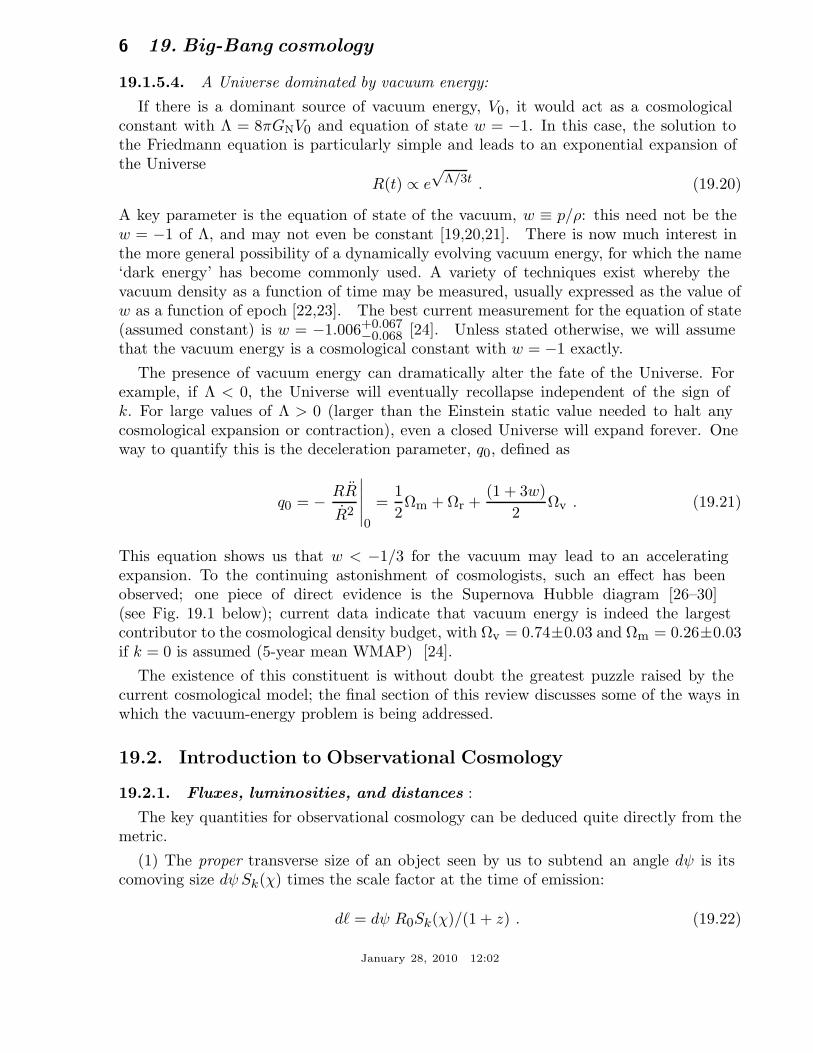
19.1.5.4. A Universe dominated by vacuum energy:

If there is a dominant source of vacuum energy, V0, it would act as a cosmologicalconstant with Λ = 8πGNV0 and equation of state w = −1. In this case, the solution tothe Friedmann equation is particularly simple and leads to an exponential expansion ofthe Universe

R(t) ∝ e√

Λ/3t . (19.20)

A key parameter is the equation of state of the vacuum, w ≡ p/ρ: this need not be thew = −1 of Λ, and may not even be constant [19,20,21]. There is now much interest inthe more general possibility of a dynamically evolving vacuum energy, for which the name‘dark energy’ has become commonly used. A variety of techniques exist whereby thevacuum density as a function of time may be measured, usually expressed as the value ofw as a function of epoch [22,23]. The best current measurement for the equation of state(assumed constant) is w = −1.006+0.067

−0.068 [24]. Unless stated otherwise, we will assumethat the vacuum energy is a cosmological constant with w = −1 exactly.

The presence of vacuum energy can dramatically alter the fate of the Universe. Forexample, if Λ < 0, the Universe will eventually recollapse independent of the sign ofk. For large values of Λ > 0 (larger than the Einstein static value needed to halt anycosmological expansion or contraction), even a closed Universe will expand forever. Oneway to quantify this is the deceleration parameter, q0, defined as

q0 = − RR

R2

∣∣∣∣∣0

=12Ωm + Ωr +

(1 + 3w)2

Ωv . (19.21)

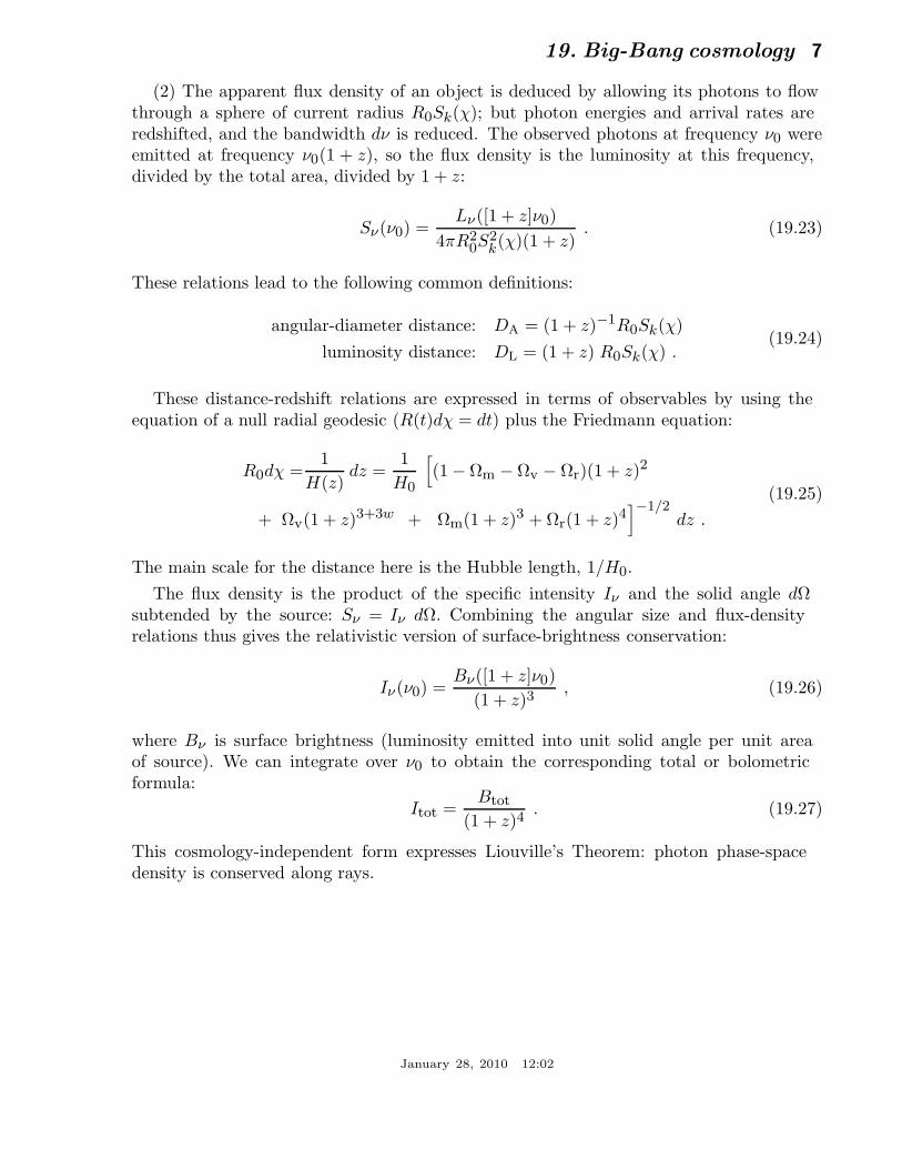
This equation shows us that w < −1/3 for the vacuum may lead to an acceleratingexpansion. To the continuing astonishment of cosmologists, such an effect has beenobserved; one piece of direct evidence is the Supernova Hubble diagram [26–30](see Fig. 19.1 below); current data indicate that vacuum energy is indeed the largestcontributor to the cosmological density budget, with Ωv = 0.74±0.03 and Ωm = 0.26±0.03if k = 0 is assumed (5-year mean WMAP) [24].

The existence of this constituent is without doubt the greatest puzzle raised by thecurrent cosmological model; the final section of this review discusses some of the ways inwhich the vacuum-energy problem is being addressed.

19.2. Introduction to Observational Cosmology

19.2.1. Fluxes, luminosities, and distances :

The key quantities for observational cosmology can be deduced quite directly from themetric.

(1) The proper transverse size of an object seen by us to subtend an angle dψ is itscomoving size dψ Sk(χ) times the scale factor at the time of emission:

d = dψ R0Sk(χ)/(1 + z) . (19.22)

January 28, 2010 12:02


(2) The apparent flux density of an object is deduced by allowing its photons to flowthrough a sphere of current radius R0Sk(χ); but photon energies and arrival rates areredshifted, and the bandwidth dν is reduced. The observed photons at frequency ν0 wereemitted at frequency ν0(1 + z), so the flux density is the luminosity at this frequency,divided by the total area, divided by 1 + z:

Sν(ν0) =Lν([1 + z]ν0)

4πR20S

2k(χ)(1 + z)

. (19.23)

These relations lead to the following common definitions:

angular-diameter distance: DA = (1 + z)−1R0Sk(χ)luminosity distance: DL = (1 + z) R0Sk(χ) .

(19.24)

These distance-redshift relations are expressed in terms of observables by using theequation of a null radial geodesic (R(t)dχ = dt) plus the Friedmann equation:

R0dχ =1

H(z)dz =

1H0

[(1 − Ωm − Ωv − Ωr)(1 + z)2

+ Ωv(1 + z)3+3w + Ωm(1 + z)3 + Ωr(1 + z)4]−1/2

dz .

(19.25)

The main scale for the distance here is the Hubble length, 1/H0.The flux density is the product of the specific intensity Iν and the solid angle dΩ

subtended by the source: Sν = Iν dΩ. Combining the angular size and flux-densityrelations thus gives the relativistic version of surface-brightness conservation:

Iν(ν0) =Bν([1 + z]ν0)

(1 + z)3, (19.26)

where Bν is surface brightness (luminosity emitted into unit solid angle per unit areaof source). We can integrate over ν0 to obtain the corresponding total or bolometricformula:

Itot =Btot

(1 + z)4. (19.27)

This cosmology-independent form expresses Liouville’s Theorem: photon phase-spacedensity is conserved along rays.

January 28, 2010 12:02


Figure 19.1: The type Ia supernova Hubble diagram [26–28]. The first panelshows that for z 1 the large-scale Hubble flow is indeed linear and uniform;the second panel shows an expanded scale, with the linear trend divided out, andwith the redshift range extended to show how the Hubble law becomes nonlinear.(Ωr = 0 is assumed.) Comparison with the prediction of Friedmann-Lemaıtremodels appears to favor a vacuum-dominated Universe.

January 28, 2010 12:02


19.2.2. Distance data and geometrical tests of cosmology :

In order to confront these theoretical predictions with data, we have to bridge thedivide between two extremes. Nearby objects may have their distances measured quiteeasily, but their radial velocities are dominated by deviations from the ideal Hubbleflow, which typically have a magnitude of several hundred km s−1. On the other hand,objects at redshifts z >∼ 0.01 will have observed recessional velocities that differ fromtheir ideal values by <∼ 10%, but absolute distances are much harder to supply in thiscase. The traditional solution to this problem is the construction of the distance ladder:an interlocking set of methods for obtaining relative distances between various classes ofobject, which begins with absolute distances at the 10 to 100 pc level, and terminateswith galaxies at significant redshifts. This is reviewed in the review on CosmologicalParameters—Sec. 21 of this Review.

By far the most exciting development in this area has been the use of type IaSupernovae (SNe), which now allow measurement of relative distances with 5% precision.In combination with Cepheid data from the HST and a direct geometrical distance tothe maser galaxy NGC4258, SNe results extend the distance ladder to the point wheredeviations from uniform expansion are negligible, leading to the best existing directvalue for H0: 74.2 ± 3.6 km s−1Mpc−1 [25]. Better still, the analysis of high-z SNehas allowed the first meaningful test of cosmological geometry to be carried out: asshown in Fig. 19.1 and Fig. 19.2, a combination of supernova data and measurements ofmicrowave-background anisotropies strongly favors a k = 0 model dominated by vacuumenergy. (See the review on Cosmological Parameters—Sec. 21 of this Review for a morecomprehensive review of Hubble parameter determinations.)

19.2.3. Age of the Universe :

The most striking conclusion of relativistic cosmology is that the Universe has notexisted forever. The dynamical result for the age of the Universe may be written as

H0t0 =∫ ∞

0

dz

(1 + z)H(z)

=∫ ∞

0

dz

(1 + z) [(1 + z)2(1 + Ωmz) − z(2 + z)Ωv]1/2, (19.28)

where we have neglected Ωr and chosen w = −1. Over the range of interest (0.1 <∼ Ωm<∼ 1,

|Ωv| <∼ 1), this exact answer may be approximated to a few % accuracy by

H0t0 23 (0.7Ωm + 0.3 − 0.3Ωv)−0.3 . (19.29)

For the special case that Ωm + Ωv = 1, the integral in Eq. (19.28) can be expressedanalytically as

H0t0 =2

3√

Ωvln

1 +√

Ωv√1 − Ωv

(Ωm < 1) . (19.30)

January 28, 2010 12:02


The most accurate means of obtaining ages for astronomical objects is based on thenatural clocks provided by radioactive decay. The use of these clocks is complicated bya lack of knowledge of the initial conditions of the decay. In the Solar System, chemicalfractionation of different elements helps pin down a precise age for the pre-Solar nebulaof 4.6 Gyr, but for stars it is necessary to attempt an a priori calculation of the relativeabundances of nuclei that result from supernova explosions. In this way, a lower limit forthe age of stars in the local part of the Milky Way of about 11 Gyr is obtained [34,35].

The other major means of obtaining cosmological age estimates is based on the theoryof stellar evolution. In principle, the main-sequence turnoff point in the color-magnitudediagram of a globular cluster should yield a reliable age. However, these have beencontroversial owing to theoretical uncertainties in the evolution model, as well asobservational uncertainties in the distance, dust extinction, and metallicity of clusters.The present consensus favors ages for the oldest clusters of about 12 Gyr [36,37].

These methods are all consistent with the age deduced from studies of structureformation, using the microwave background and large-scale structure: t0 = 13.69 ±0.13 Gyr [24], where the extra accuracy comes at the price of assuming the Cold DarkMatter model to be true.

19.2.4. Horizon, isotropy, flatness problems :

For photons, the radial equation of motion is just c dt = R dχ. How far can a photonget in a given time? The answer is clearly

∆χ =∫ t2

t1

dt

R(t)≡ ∆η , (19.31)

i.e., just the interval of conformal time. We can replace dt by dR/R, which the Friedmannequation says is ∝ dR/

√ρR2 at early times. Thus, this integral converges if ρR2 → ∞ as

t1 → 0, otherwise it diverges. Provided the equation of state is such that ρ changes fasterthan R−2, light signals can only propagate a finite distance between the Big Bang andthe present; there is then said to be a particle horizon. Such a horizon therefore existsin conventional Big-Bang models, which are dominated by radiation (ρ ∝ R−4) at earlytimes.

At late times, the integral for the horizon is largely determined by the matter-dominatedphase, for which

DH = R0 χH≡ R0

∫ t(z)

0

dt

R(t) 6000√

Ωzh−1 Mpc (z 1) . (19.32)

The horizon at the time of formation of the microwave background (‘last scattering:’z 1100) was thus of order 100 Mpc in size, subtending an angle of about 1. Why thenare the large number of causally disconnected regions we see on the microwave sky allat the same temperature? The Universe is very nearly isotropic and homogeneous, eventhough the initial conditions appear not to permit such a state to be constructed.

January 28, 2010 12:02


WMAP

SNLS

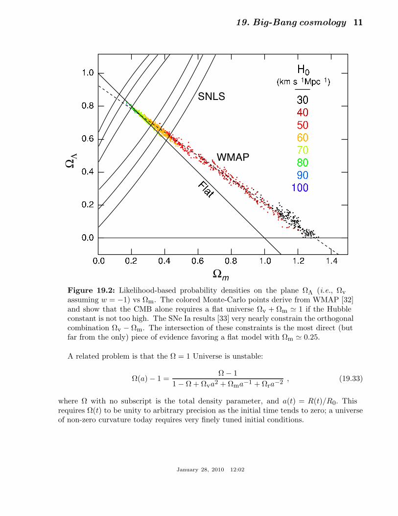
Figure 19.2: Likelihood-based probability densities on the plane ΩΛ (i.e., Ωv

assuming w = −1) vs Ωm. The colored Monte-Carlo points derive from WMAP [32]and show that the CMB alone requires a flat universe Ωv + Ωm 1 if the Hubbleconstant is not too high. The SNe Ia results [33] very nearly constrain the orthogonalcombination Ωv − Ωm. The intersection of these constraints is the most direct (butfar from the only) piece of evidence favoring a flat model with Ωm 0.25.

A related problem is that the Ω = 1 Universe is unstable:

Ω(a) − 1 =Ω − 1

1 − Ω + Ωva2 + Ωma−1 + Ωra−2, (19.33)

where Ω with no subscript is the total density parameter, and a(t) = R(t)/R0. Thisrequires Ω(t) to be unity to arbitrary precision as the initial time tends to zero; a universeof non-zero curvature today requires very finely tuned initial conditions.

January 28, 2010 12:02


19.3. The Hot Thermal Universe

19.3.1. Thermodynamics of the early Universe :As alluded to above, we expect that much of the early Universe can be described by

a radiation-dominated equation of state. In addition, through much of the radiation-dominated period, thermal equilibrium is established by the rapid rate of particleinteractions relative to the expansion rate of the Universe (see Sec. 19.3.3 below). Inequilibrium, it is straightforward to compute the thermodynamic quantities, ρ, p, andthe entropy density, s. In general, the energy density for a given particle type i can bewritten as

ρi =∫

Ei dnqi , (19.34)

with the density of states given by

dnqi =gi

2π2

(exp[(Eqi − µi)/Ti] ± 1

)−1q2i dqi , (19.35)

where gi counts the number of degrees of freedom for particle type i, E2qi

= m2i + q2

i ,µi is the chemical potential, and the ± corresponds to either Fermi or Bose statistics.Similarly, we can define the pressure of a perfect gas as

pi =13

∫q2i

Eidnqi . (19.36)

The number density of species i is simply

ni =∫

dnqi , (19.37)

and the entropy density is

si =ρi + pi − µini

Ti. (19.38)

In the Standard Model, a chemical potential is often associated with baryon number,and since the net baryon density relative to the photon density is known to be verysmall (of order 10−10), we can neglect any such chemical potential when computing totalthermodynamic quantities.

For photons, we can compute all of the thermodynamic quantities rather easily. Takinggi = 2 for the 2 photon polarization states, we have (in units where = kB = 1)

ργ =π2

15T 4 ; pγ =

13ργ ; sγ =

4ργ

3T; nγ =

2ζ(3)π2

T 3 , (19.39)

with 2ζ(3)/π2 0.2436. Note that Eq. (19.10) can be converted into an equation forentropy conservation. Recognizing that p = sT , Eq. (19.10) becomes

d(sR3)/dt = 0 . (19.40)

For radiation, this corresponds to the relationship between expansion and cooling,T ∝ R−1 in an adiabatically expanding universe. Note also that both s and nγ scale asT 3.

January 28, 2010 12:02


19.3.2. Radiation content of the Early Universe :At the very high temperatures associated with the early Universe, massive particles

are pair produced, and are part of the thermal bath. If for a given particle species iwe have T mi, then we can neglect the mass in Eq. (19.34) to Eq. (19.38), and thethermodynamic quantities are easily computed as in Eq. (19.39). In general, we canapproximate the energy density (at high temperatures) by including only those particleswith mi T . In this case, we have

ρ =

(∑B

gB +78

∑F

gF

)π2

30T 4 ≡ π2

30N(T ) T 4 , (19.41)

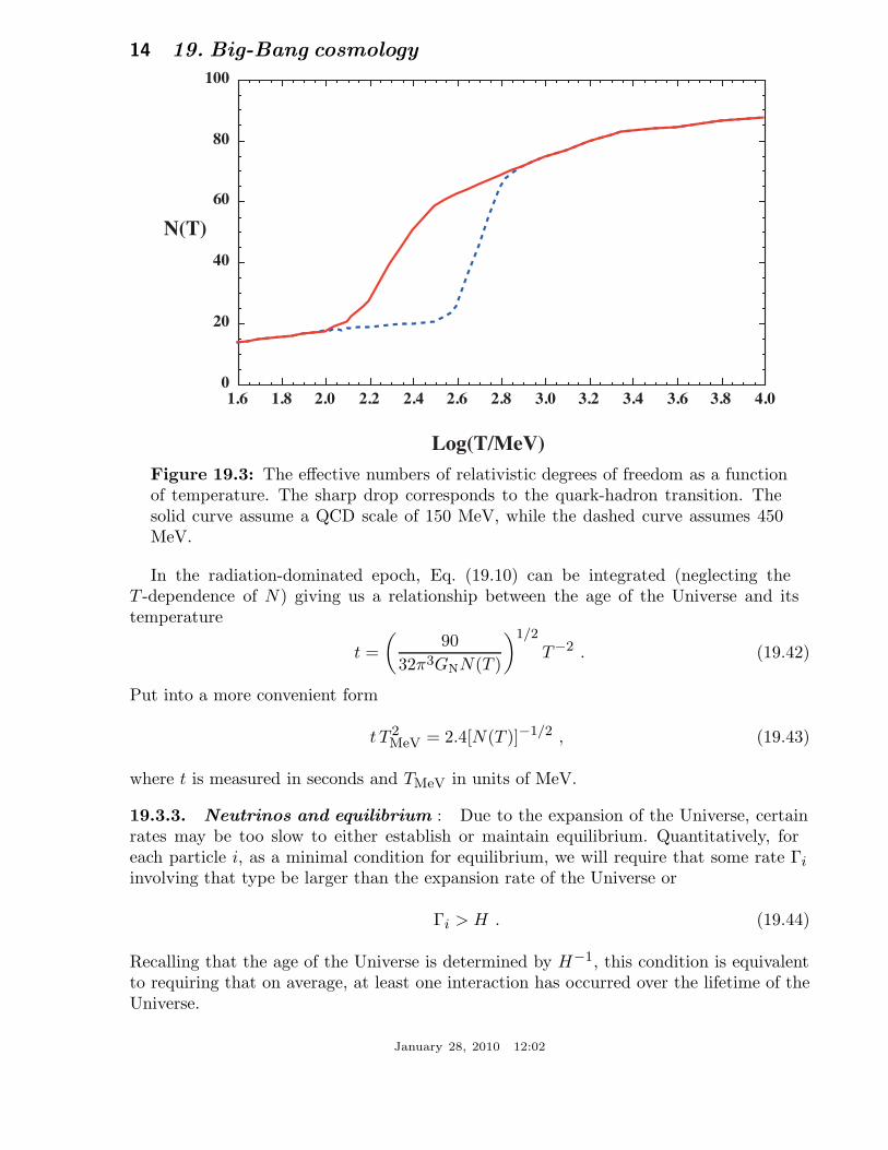
where gB(F ) is the number of degrees of freedom of each boson (fermion) and the sumruns over all boson and fermion states with m T . The factor of 7/8 is due to thedifference between the Fermi and Bose integrals. Eq. (19.41) defines the effective numberof degrees of freedom, N(T ), by taking into account new particle degrees of freedom asthe temperature is raised. This quantity is plotted in Fig. 19.3 [38].

The value of N(T ) at any given temperature depends on the particle physics model.In the standard SU(3)× SU(2)×U(1) model, we can specify N(T ) up to temperatures ofO(100) GeV. The change in N (ignoring mass effects) can be seen in the above table.

Temperature New Particles 4N(T )T < me γ’s + ν’s 29me < T < mµ e± 43mµ < T < mπ µ± 57mπ < T < T

†c π’s 69

Tc < T < mstrange π’s + u, u, d, d + gluons 205ms < T < mcharm s, s 247mc < T < mτ c, c 289mτ < T < mbottom τ± 303mb < T < mW,Z b, b 345mW,Z < T < mHiggs W±, Z 381mH < T < mtop H0 385mt < T t, t 427

†Tc corresponds to the confinement-deconfinement transition between quarks and hadrons.

At higher temperatures, N(T ) will be model-dependent. For example, in the minimalSU(5) model, one needs to add 24 states to N(T ) for the X and Y gauge bosons, another24 from the adjoint Higgs, and another 6 (in addition to the 4 already counted in W±, Z,and H) from the 5 of Higgs. Hence for T > mX in minimal SU(5), N(T ) = 160.75. In asupersymmetric model this would at least double, with some changes possibly necessaryin the table if the lightest supersymmetric particle has a mass below mt.

January 28, 2010 12:02


0

20

40

60

80

100

1.6 1.8 2.0 2.2 2.4 2.6 2.8 3.0 3.2 3.4 3.6 3.8 4.0

N(T)

Log(T/MeV)Figure 19.3: The effective numbers of relativistic degrees of freedom as a functionof temperature. The sharp drop corresponds to the quark-hadron transition. Thesolid curve assume a QCD scale of 150 MeV, while the dashed curve assumes 450MeV.

In the radiation-dominated epoch, Eq. (19.10) can be integrated (neglecting theT -dependence of N) giving us a relationship between the age of the Universe and itstemperature

t =(

9032π3GNN(T )

)1/2

T−2 . (19.42)

Put into a more convenient form

t T 2MeV = 2.4[N(T )]−1/2 , (19.43)

where t is measured in seconds and TMeV in units of MeV.

19.3.3. Neutrinos and equilibrium : Due to the expansion of the Universe, certainrates may be too slow to either establish or maintain equilibrium. Quantitatively, foreach particle i, as a minimal condition for equilibrium, we will require that some rate Γi

involving that type be larger than the expansion rate of the Universe or

Γi > H . (19.44)

Recalling that the age of the Universe is determined by H−1, this condition is equivalentto requiring that on average, at least one interaction has occurred over the lifetime of theUniverse.

January 28, 2010 12:02


A good example for a process which goes in and out of equilibrium is the weakinteractions of neutrinos. On dimensional grounds, one can estimate the thermallyaveraged scattering cross section

〈σv〉 ∼ O(10−2)T 2/m4W (19.45)

for T <∼ mW. Recalling that the number density of leptons is n ∝ T 3, we can comparethe weak interaction rate, Γwk ∼ n〈σv〉, with the expansion rate,

H =(

8πGNρ

3

)1/2

=(

8π3

90N(T )

)1/2

T 2/MP

∼ 1.66N(T )1/2T 2/MP,

(19.46)

where the Planck mass MP = G−1/2N = 1.22 × 1019 GeV.

Neutrinos will be in equilibrium when Γwk > H or

T > (500 m4W/MP)1/3 ∼ 1 MeV . (19.47)

However, this condition assumes T mW; for higher temperatures, we should write〈σv〉 ∼ O(10−2)/T 2, so that Γ ∼ 10−2T . Thus, in the very early stages of expansion, attemperatures T >∼ 10−2MP/

√N , equilibrium will not have been established.

Having attained a quasi-equilibrium stage, the Universe then cools further to thepoint where the interaction and expansion timescales match once again. The temperatureat which these rates are equal is commonly referred to as the neutrino decoupling orfreeze-out temperature and is defined by Γwk(Td) = H(Td). For T < Td, neutrinos dropout of equilibrium. The Universe becomes transparent to neutrinos and their momentasimply redshift with the cosmic expansion. The effective neutrino temperature will simplyfall with T ∼ 1/R.

Soon after decoupling, e± pairs in the thermal background begin to annihilate (whenT <∼ me). Because the neutrinos are decoupled, the energy released due to annihilationheats up the photon background relative to the neutrinos. The change in the photontemperature can be easily computed from entropy conservation. The neutrino entropymust be conserved separately from the entropy of interacting particles. A straightforwardcomputation yields

Tν = (4/11)1/3 Tγ 1.9 K . (19.48)

Today, the total entropy density is therefore given by

s =43

π2

30

(2 +

214

(Tν/Tγ)3)

T 3γ =

43

π2

30

(2 +

2111

)T 3

γ = 7.04 nγ . (19.49)

Similarly, the total relativistic energy density today is given by

ρr =π2

30

[2 +

214

(Tν/Tγ)4]

T 4γ 1.68ργ . (19.50)

January 28, 2010 12:02


In practice, a small correction is needed to this, since neutrinos are not totallydecoupled at e± annihilation: the effective number of massless neutrino species is 3.04,rather than 3 [39].

This expression ignores neutrino rest masses, but current oscillation data requireat least one neutrino eigenstate to have a mass exceeding 0.05 eV. In this minimalcase, Ωνh2 = 5 × 10−4, so the neutrino contribution to the matter budget would benegligibly small (which is our normal assumption). However, a nearly degenerate patternof mass eigenstates could allow larger densities, since oscillation experiments only measuredifferences in m2 values. Note that a 0.05-eV neutrino has kTν = mν at z 297, so theabove expression for the total present relativistic density is really only an extrapolation.However, neutrinos are almost certainly relativistic at all epochs where the radiationcontent of the Universe is dynamically significant.

19.3.4. Field Theory and Phase transitions :It is very likely that the Universe has undergone one or more phase transitions during

the course of its evolution [40–43]. Our current vacuum state is described by SU(3)c×U(1)em, which in the Standard Model is a remnant of an unbroken SU(3)c× SU(2)L×U(1)Y gauge symmetry. Symmetry breaking occurs when a non-singlet gauge field (theHiggs field in the Standard Model) picks up a non-vanishing vacuum expectation value,determined by a scalar potential. For example, a simple (non-gauged) potential describingsymmetry breaking is V (φ) = 1

4λφ4 − 12µ2φ2 + V (0). The resulting expectation value is

simply 〈φ〉 = µ/√

λ.In the early Universe, finite temperature radiative corrections typically add terms

to the potential of the form φ2T 2. Thus, at very high temperatures, the symmetry isrestored and 〈φ〉 = 0. As the Universe cools, depending on the details of the potential,symmetry breaking will occur via a first order phase transition in which the field tunnelsthrough a potential barrier, or via a second order transition in which the field evolvessmoothly from one state to another (as would be the case for the above examplepotential).

The evolution of scalar fields can have a profound impact on the early Universe. Theequation of motion for a scalar field φ can be derived from the energy-momentum tensor

Tµν = ∂µφ∂νφ − 12gµν∂ρφ∂ρφ − gµνV (φ) . (19.51)

By associating ρ = T00 and p = R−2(t)Tii we have

ρ =12φ2 +

12R−2(t)(∇φ)2 + V (φ)

p =12φ2 − 1

6R−2(t)(∇φ)2 − V (φ) ,

(19.52)

and from Eq. (19.10) we can write the equation of motion (by considering a homogeneousregion, we can ignore the gradient terms)

φ + 3Hφ = −∂V/∂φ . (19.53)

January 28, 2010 12:02


19.3.5. Inflation :In Sec. 19.2.4, we discussed some of the problems associated with the standard

Big-Bang model. However, during a phase transition, our assumptions of an adiabaticallyexpanding universe are generally not valid. If, for example, a phase transition occurredin the early Universe such that the field evolved slowly from the symmetric state to theglobal minimum, the Universe may have been dominated by the vacuum energy densityassociated with the potential near φ ≈ 0. During this period of slow evolution, the energydensity due to radiation will fall below the vacuum energy density, ρ V (0). When thishappens, the expansion rate will be dominated by the constant V(0), and we obtain theexponentially expanding solution given in Eq. (19.20). When the field evolves towardsthe global minimum it will begin to oscillate about the minimum, energy will be releasedduring its decay, and a hot thermal universe will be restored. If released fast enough, itwill produce radiation at a temperature NTR

4 <∼ V (0). In this reheating process, entropyhas been created and the final value of R T is greater than the initial value of R T . Thus,we see that, during a phase transition, the relation R T ∼ constant need not hold true.This is the basis of the inflationary Universe scenario [44–46].

If, during the phase transition, the value of R T changed by a factor of O(1029), thecosmological problems discussed above would be solved. The observed isotropy would begenerated by the immense expansion; one small causal region could get blown up, andhence, our entire visible Universe would have been in thermal contact some time in thepast. In addition, the density parameter Ω would have been driven to 1 (with exponentialprecision). Density perturbations will be stretched by the expansion, λ ∼ R(t). Thus itwill appear that λ H−1 or that the perturbations have left the horizon, where in factthe size of the causally connected region is now no longer simply H−1. However, not onlydoes inflation offer an explanation for large scale perturbations, it also offers a source forthe perturbations themselves through quantum fluctuations.

Early models of inflation were based on a first order phase transition of a GrandUnified Theory [47]. Although these models led to sufficient exponential expansion,completion of the transition through bubble percolation did not occur. Later models ofinflation [48,49], also based on Grand Unified symmetry breaking, through second ordertransitions were also doomed. While they successfully inflated and reheated, and in factproduced density perturbations due to quantum fluctuations during the evolution of thescalar field, they predicted density perturbations many orders of magnitude too large.Most models today are based on an unknown symmetry breaking involving a new scalarfield, the inflaton, φ.

19.3.6. Baryogenesis :The Universe appears to be populated exclusively with matter rather than antimatter.

Indeed antimatter is only detected in accelerators or in cosmic rays. However, thepresence of antimatter in the latter is understood to be the result of collisions of primaryparticles in the interstellar medium. There is in fact strong evidence against primaryforms of antimatter in the Universe. Furthermore, the density of baryons compared tothe density of photons is extremely small, η ∼ 10−10.

The production of a net baryon asymmetry requires baryon number violating

January 28, 2010 12:02


interactions, C and CP violation and a departure from thermal equilibrium [50]. Thefirst two of these ingredients are expected to be contained in grand unified theories aswell as in the non-perturbative sector of the Standard Model, the third can be realized inan expanding universe where as we have seen interactions come in and out of equilibrium.

There are several interesting and viable mechanisms for the production of the baryonasymmetry. While, we can not review any of them here in any detail, we mentionsome of the important scenarios. In all cases, all three ingredients listed above areincorporated. One of the first mechanisms was based on the out of equilibrium decay ofa massive particle such as a superheavy GUT gauge of Higgs boson [51,52]. A novelmechanism involving the decay of flat directions in supersymmetric models is known as theAffleck-Dine scenario [53]. Recently, much attention has been focused on the possibilityof generating the baryon asymmetry at the electro-weak scale using the non-perturbativeinteractions of sphalerons [54]. Because these interactions conserve the sum of baryonand lepton number, B + L, it is possible to first generate a lepton asymmetry (e.g., bythe out-of-equilibrium decay of a superheavy right-handed neutrino), which is convertedto a baryon asymmetry at the electro-weak scale [55]. This mechanism is known aslepto-baryogenesis.

19.3.7. Nucleosynthesis :An essential element of the standard cosmological model is Big-Bang nucleosynthesis

(BBN), the theory which predicts the abundances of the light element isotopes D, 3He,4He, and 7Li. Nucleosynthesis takes place at a temperature scale of order 1 MeV. Thenuclear processes lead primarily to 4He, with a primordial mass fraction of about 25%.Lesser amounts of the other light elements are produced: about 10−5 of D and 3He andabout 10−10 of 7Li by number relative to H. The abundances of the light elements dependalmost solely on one key parameter, the baryon-to-photon ratio, η. The nucleosynthesispredictions can be compared with observational determinations of the abundances ofthe light elements. Consistency between theory and observations leads to a conservativerange of

5.1 × 10−10 < η < 6.5 × 10−10 . (19.54)

η is related to the fraction of Ω contained in baryons, Ωb

Ωb = 3.66 × 107η h−2 , (19.55)

or 1010η = 274Ωbh2. The WMAP result [24] for Ωbh2 of 0.0227 ± 0.0006 translatesinto a value of η = 6.23 ± 0.17. This result can be used to ‘predict’ the light elementabundance which can in turn be compared with observation [56]. The resulting D/Habundance is in excellent agreement with that found in quasar absorption systems. Itis in reasonable agreement with the helium abundance observed in extra-galactic HIIregions (once systematic uncertainties are accounted for), but is in poor agreement withthe Li abundance observed in the atmospheres of halo dwarf stars [57]. (See the reviewon BBN—Sec. 20 of this Review for a detailed discussion of BBN or references [58,59]. )

January 28, 2010 12:02


19.3.8. The transition to a matter-dominated Universe :In the Standard Model, the temperature (or redshift) at which the Universe undergoes

a transition from a radiation dominated to a matter dominated Universe is determined bythe amount of dark matter. Assuming three nearly massless neutrinos, the energy densityin radiation at temperatures T 1 MeV, is given by

ρr =π2

30

[2 +

214

(411

)4/3]

T 4 . (19.56)

In the absence of non-baryonic dark matter, the matter density can be written as

ρm = mNη nγ , (19.57)

where mN is the nucleon mass. Recalling that nγ ∝ T 3 [cf. Eq. (19.39)], we can solve forthe temperature or redshift at the matter-radiation equality when ρr = ρm,

Teq = 0.22 mN η or (1 + zeq) = 0.22 ηmN

T0, (19.58)

where T0 is the present temperature of the microwave background. For η = 6.2 × 10−10,this corresponds to a temperature Teq 0.13 eV or (1+ zeq) 550. A transition this lateis very problematic for structure formation (see Sec. 19.4.5).

The redshift of matter domination can be pushed back significantly if non-baryonicdark matter is present. If instead of Eq. (19.57), we write

ρm = Ωmρc

(T

T0

)3

, (19.59)

we find thatTeq = 0.9

Ωmρc

T 30

or (1 + zeq) = 2.4 × 104Ωmh2 . (19.60)

19.4. The Universe at late times

19.4.1. The CMB :One form of the infamous Olbers’ paradox says that, in Euclidean space, surface

brightness is independent of distance. Every line of sight will terminate on matter thatis hot enough to be ionized and so scatter photons: T >∼ 103 K; the sky should thereforeshine as brightly as the surface of the Sun. The reason the night sky is dark is entirelydue to the expansion, which cools the radiation temperature to 2.73 K. This gives aPlanck function peaking at around 1 mm to produce the microwave background (CMB).

The CMB spectrum is a very accurate match to a Planck function [60]. (See thereview on CBR–Sec. 23 of this Review.) The COBE estimate of the temperature is [61]

T = 2.725 ± 0.001 K . (19.61)

January 28, 2010 12:02


The lack of any distortion of the Planck spectrum is a strong physical constraint. It isvery difficult to account for in any expanding universe other than one that passes througha hot stage. Alternative schemes for generating the radiation, such as thermalizationof starlight by dust grains, inevitably generate a superposition of temperatures. Whatis required in addition to thermal equilibrium is that T ∝ 1/R, so that radiation fromdifferent parts of space appears identical.

Although it is common to speak of the CMB as originating at “recombination,” amore accurate terminology is the era of “last scattering.” In practice, this takes placeat z 1100, almost independently of the main cosmological parameters, at which timethe fractional ionization is very small. This occurred when the age of the Universe wasa few hundred thousand years. (See the review on CBR–Sec. 23 of this Review for a fulldiscussion of the CMB.)

19.4.2. Matter in the Universe :One of the main tasks of cosmology is to measure the density of the Universe, and

how this is divided between dark matter and baryons. The baryons consist partly ofstars, with 0.002 <∼ Ω∗ <∼ 0.003 [62] but mainly inhabit the intergalactic medium (IGM).One powerful way in which this can be studied is via the absorption of light fromdistant luminous objects such as quasars. Even very small amounts of neutral hydrogencan absorb rest-frame UV photons (the Gunn-Peterson effect), and should suppress thecontinuum by a factor exp(−τ), where

τ 104.62h−1

[nHI(z)/m−3

(1 + z)√

1 + Ωmz

], (19.62)

and this expression applies while the Universe is matter dominated (z >∼ 1 in theΩm = 0.3 Ωv = 0.7 model). It is possible that this general absorption has now been seenat z = 6.2 − 6.4 [63]. In any case, the dominant effect on the spectrum is a ‘forest’ ofnarrow absorption lines, which produce a mean τ = 1 in the Lyα forest at about z = 3,and so we have ΩHI 10−6.7h−1. This is such a small number that clearly the IGM isvery highly ionized at these redshifts.

The Lyα forest is of great importance in pinning down the abundance of deuterium.Because electrons in deuterium differ in reduced mass by about 1 part in 4000 comparedto hydrogen, each absorption system in the Lyα forest is accompanied by an offsetdeuterium line. By careful selection of systems with an optimal HI column density, ameasurement of the D/H ratio can be made. This has now been done in 7 quasars,with relatively consistent results [64]. Combining these determinations with the theoryof primordial nucleosynthesis yields a baryon density of Ωbh2 = 0.019 − 0.024 (95%confidence). (See also the review on BBN—Sec. 20 of this Review.)

Ionized IGM can also be detected in emission when it is densely clumped, viabremsstrahlung radiation. This generates the spectacular X-ray emission from richclusters of galaxies. Studies of this phenomenon allow us to achieve an accounting of thetotal baryonic material in clusters. Within the central 1 Mpc, the masses in stars,X-ray emitting gas and total dark matter can be determined with reasonable accuracy

January 28, 2010 12:02


(perhaps 20% rms), and this allows a minimum baryon fraction to be determined [65,66]:

Mbaryons

Mtotal

>∼ 0.009 + (0.066 ± 0.003) h−3/2 . (19.63)

Because clusters are the largest collapsed structures, it is reasonable to take this asapplying to the Universe as a whole. This equation implies a minimum baryon fraction ofperhaps 12% (for reasonable h), which is too high for Ωm = 1 if we take Ωbh2 0.02 fromnucleosynthesis. This is therefore one of the more robust arguments in favor of Ωm 0.3.(See the review on Cosmological Parameters—Sec. 21 of this Review.) This argument isalso consistent with the inference on Ωm that can be made from Fig. 19.2.

This method is much more robust than the older classical technique for weighingthe Universe: ‘L × M/L.’ The overall light density of the Universe is reasonably welldetermined from redshift surveys of galaxies, so that a good determination of mass Mand luminosity L for a single object suffices to determine Ωm if the mass-to-light ratio isuniversal.

19.4.3. Gravitational lensing :A robust method for determining masses in cosmology is to use gravitational light

deflection. Most systems can be treated as a geometrically thin gravitational lens, wherethe light bending is assumed to take place only at a single distance. Simple geometrythen determines a mapping between the coordinates in the intrinsic source plane and theobserved image plane:

α(DLθI) =DS

DLS(θI − θS) , (19.64)

where the angles θI, θS and α are in general two-dimensional vectors on the sky. Thedistances DLS etc. are given by an extension of the usual distance-redshift formula:

DLS =R0Sk(χS − χL)

1 + zS. (19.65)

This is the angular-diameter distance for objects on the source plane as perceived by anobserver on the lens.

Solutions of this equation divide into weak lensing, where the mapping between sourceplane and image plane is one-to-one, and strong lensing, in which multiple imaging ispossible. For circularly-symmetric lenses, an on-axis source is multiply imaged into a‘caustic’ ring, whose radius is the Einstein radius:

θE =(

4GMDLS

DLDS

)1/2

=(

M

1011.09M

)1/2 (DLDS/DLS

Gpc

)−1/2

arcsec .

(19.66)

The observation of ‘arcs’ (segments of near-perfect Einstein rings) in rich clusters ofgalaxies has thus given very accurate masses for the central parts of clusters—generally in

January 28, 2010 12:02


good agreement with other indicators, such as analysis of X-ray emission from the clusterIGM [67].

Gravitational lensing has also developed into a particularly promising probe ofcosmological structure on 10 to 100 Mpc scales. Weak image distortions manifestthemselves as an additional ellipticity of galaxy images (‘shear’), which can be observedby averaging many images together (the corresponding flux amplification is less readilydetected). The result is a ‘cosmic shear’ field of order 1% ellipticity, coherent overscales of around 30 arcmin, which is directly related to the cosmic mass field, withoutany astrophysical uncertainties. For this reason, weak lensing is seen as potentially thecleanest probe of matter fluctuations, next to the CMB. Already, impressive results havebeen obtained in measuring cosmological parameters, based on survey data from only∼ 10 deg2 [68]. The particular current strength of this technique is the ability to measurethe amplitude of mass fluctuations; this can be deduced from the CMB only subject touncertainty over the optical depth due to Thomson scattering after reionization.

19.4.4. Density Fluctuations :The overall properties of the Universe are very close to being homogeneous; and yet

telescopes reveal a wealth of detail on scales varying from single galaxies to large-scalestructures of size exceeding 100 Mpc. The existence of these structures must be tellingus something important about the initial conditions of the Big Bang, and about thephysical processes that have operated subsequently. This motivates the study of thedensity perturbation field, defined as

δ(x) ≡ ρ(x) − 〈ρ〉〈ρ〉 . (19.67)

A critical feature of the δ field is that it inhabits a universe that is isotropic andhomogeneous in its large-scale properties. This suggests that the statistical properties ofδ should also be statistically homogeneous—i.e., it is a stationary random process.

It is often convenient to describe δ as a Fourier superposition:

δ(x) =∑

δke−ik·x . (19.68)

We avoid difficulties with an infinite universe by applying periodic boundary conditionsin a cube of some large volume V . The cross-terms vanish when we compute the variancein the field, which is just a sum over modes of the power spectrum

〈δ2〉 =∑

|δk|2 ≡∑

P (k) . (19.69)

Note that the statistical nature of the fluctuations must be isotropic, so we write P (k)rather than P (k). The 〈. . .〉 average here is a volume average. Cosmological density fieldsare an example of an ergodic process, in which the average over a large volume tends tothe same answer as the average over a statistical ensemble.

The statistical properties of discrete objects sampled from the density field are oftendescribed in terms of N -point correlation functions, which represent the excess probability

January 28, 2010 12:02


over random for finding one particle in each of N boxes in a given configuration.For the 2-point case, the correlation function is readily shown to be identical to theautocorrelation function of the δ field: ξ(r) = 〈δ(x)δ(x + r)〉.

The power spectrum and correlation function are Fourier conjugates, and thusare equivalent descriptions of the density field (similarly, k-space equivalents existfor the higher-order correlations). It is convenient to take the limit V → ∞ anduse k-space integrals, defining a dimensionless power spectrum, which measures thecontribution to the fractional variance in density per unit logarithmic range of scale, as∆2(k) = d〈δ2〉/d lnk = V k3P (k)/2π2:

ξ(r) =∫

∆2(k)sin kr

krd ln k; ∆2(k) =

2π

k3∫ ∞

0ξ(r)

sin kr

krr2 dr . (19.70)

For many years, an adequate approximation to observational data on galaxies wasξ = (r/r0)−γ , with γ 1.8 and r0 5 h−1 Mpc. Modern surveys are now able to probeinto the large-scale linear regime where unaltered traces of the curved post-recombinationspectrum can be detected [69,70,71].

19.4.5. Formation of cosmological structure :The simplest model for the generation of cosmological structure is gravitational

instability acting on some small initial fluctuations (for the origin of which a theorysuch as inflation is required). If the perturbations are adiabatic (i.e., fractionally perturbnumber densities of photons and matter equally), the linear growth law for matterperturbations is simple:

δ ∝

a2(t) (radiation domination; Ωr = 1)a(t) (matter domination; Ωm = 1) .

(19.71)

For low density universes, the present-day amplitude is suppressed by a factor g(Ω),where

g(Ω) 52Ωm

[Ω4/7

m − Ωv + (1 + Ωm/2)(1 +170

Ωv)]−1

(19.72)

is an accurate fit for models with matter plus cosmological constant. The alternativeperturbation mode is isocurvature: only the equation of state changes, and the totaldensity is initially unperturbed. These modes perturb the total entropy density, andthus induce additional large-scale CMB anisotropies [72]. Although the character ofperturbations in the simplest inflationary theories are purely adiabatic, correlatedadiabatic and isocurvature modes are predicted in many models; the simplest example isthe curvaton, which is a scalar field that decays to yield a perturbed radiation density. Ifthe matter content already exists at this time, the overall perturbation field will have asignificant isocurvature component. Such a prediction is inconsistent with current CMBdata [73], and most analyses of CMB and LSS data assume the adiabatic case to holdexactly.

Linear evolution preserves the shape of the power spectrum. However, a variety ofprocesses mean that growth actually depends on the matter content:

January 28, 2010 12:02


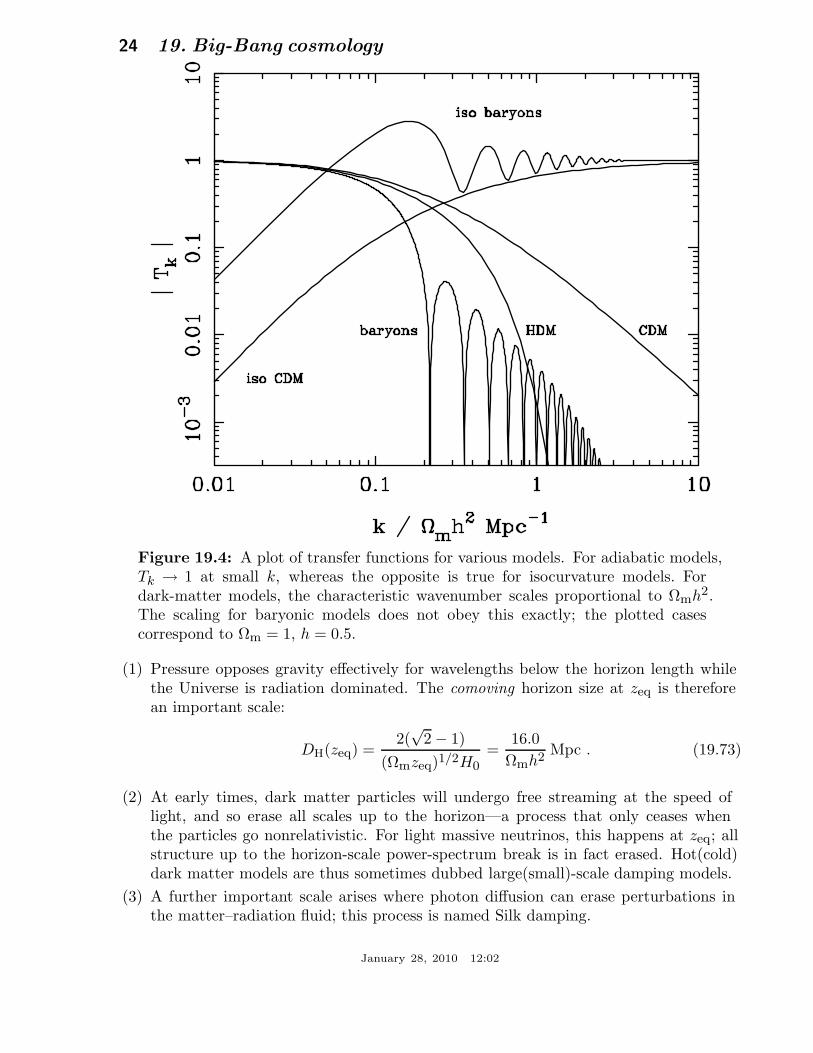
Figure 19.4: A plot of transfer functions for various models. For adiabatic models,Tk → 1 at small k, whereas the opposite is true for isocurvature models. Fordark-matter models, the characteristic wavenumber scales proportional to Ωmh2.The scaling for baryonic models does not obey this exactly; the plotted casescorrespond to Ωm = 1, h = 0.5.

(1) Pressure opposes gravity effectively for wavelengths below the horizon length whilethe Universe is radiation dominated. The comoving horizon size at zeq is thereforean important scale:

DH(zeq) =2(√

2 − 1)(Ωmzeq)1/2H0

=16.0

Ωmh2Mpc . (19.73)

(2) At early times, dark matter particles will undergo free streaming at the speed oflight, and so erase all scales up to the horizon—a process that only ceases whenthe particles go nonrelativistic. For light massive neutrinos, this happens at zeq; allstructure up to the horizon-scale power-spectrum break is in fact erased. Hot(cold)dark matter models are thus sometimes dubbed large(small)-scale damping models.

(3) A further important scale arises where photon diffusion can erase perturbations inthe matter–radiation fluid; this process is named Silk damping.

January 28, 2010 12:02


The overall effect is encapsulated in the transfer function, which gives the ratio ofthe late-time amplitude of a mode to its initial value (see Fig. 19.4). The overall powerspectrum is thus the primordial power-law, times the square of the transfer function:

P (k) ∝ kn T 2k . (19.74)

The most generic power-law index is n = 1: the ‘Zeldovich’ or ‘scale-invariant’ spectrum.Inflationary models tend to predict a small ‘tilt:’ |n − 1| <∼ 0.03 [12,13]. On theassumption that the dark matter is cold, the power spectrum then depends on 5parameters: n, h, Ωb, Ωcdm (≡ Ωm − Ωb) and an overall amplitude. The latter is oftenspecified as σ8, the linear-theory fractional rms in density when a spherical filter ofradius 8 h−1 Mpc is applied in linear theory. This scale can be probed directly via weakgravitational lensing, and also via its effect on the abundance of rich galaxy clusters. Thefavored value is approximately [32,74]

σ8 (0.803 ± 0.011) (Ωm/0.25)−0.47 . (19.75)

A direct measure of mass inhomogeneity is valuable, since the galaxies inevitably arebiased with respect to the mass. This means that the fractional fluctuations in galaxynumber, δn/n, may differ from the mass fluctuations, δρ/ρ. It is commonly assumed thatthe two fields obey some proportionality on large scales where the fluctuations are small,δn/n = bδρ/ρ, but even this is not guaranteed [75].

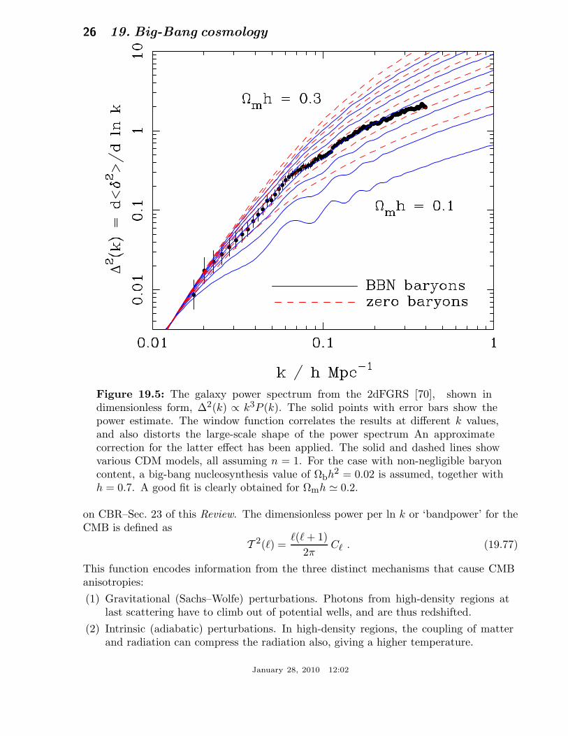
The main shape of the transfer function is a break around the horizon scale atzeq, which depends just on Ωmh when wavenumbers are measured in observable units( h Mpc−1). For reasonable baryon content, weak oscillations in the transfer function arealso expected, and these BAOs (Baryon Acoustic Oscillations) have been clearly detected[76,77]. As well as directly measuring the baryon fraction, the scale of the oscillationsdirectly measures the acoustic horizon at decoupling; this can be used as an additionalstandard ruler for cosmological tests, and the BAO method is likely to be importantin future large galaxy surveys. Overall, current power-spectrum data [69,70,71] favorΩmh 0.20 and a baryon fraction of about 0.15 for n = 1 (see Fig. 19.5).

In principle, accurate data over a wide range of k could determine both Ωh and n, butin practice there is a strong degeneracy between these. In order to constrain n itself, it isnecessary to examine data on anisotropies in the CMB.

19.4.6. CMB anisotropies :

The CMB has a clear dipole anisotropy, of magnitude 1.23 × 10−3. This is interpretedas being due to the Earth’s motion, which is equivalent to a peculiar velocity for theMilky Way of

vMW 600 km s−1 towards (, b) (270, 30) . (19.76)

All higher-order multipole moments of the CMB are however much smaller (of order10−5), and interpreted as signatures of density fluctuations at last scattering ( 1100).To analyze these, the sky is expanded in spherical harmonics as explained in the review

January 28, 2010 12:02


Figure 19.5: The galaxy power spectrum from the 2dFGRS [70], shown indimensionless form, ∆2(k) ∝ k3P (k). The solid points with error bars show thepower estimate. The window function correlates the results at different k values,and also distorts the large-scale shape of the power spectrum An approximatecorrection for the latter effect has been applied. The solid and dashed lines showvarious CDM models, all assuming n = 1. For the case with non-negligible baryoncontent, a big-bang nucleosynthesis value of Ωbh2 = 0.02 is assumed, together withh = 0.7. A good fit is clearly obtained for Ωmh 0.2.

on CBR–Sec. 23 of this Review. The dimensionless power per ln k or ‘bandpower’ for theCMB is defined as

T 2() =( + 1)

2πC . (19.77)

This function encodes information from the three distinct mechanisms that cause CMBanisotropies:(1) Gravitational (Sachs–Wolfe) perturbations. Photons from high-density regions at

last scattering have to climb out of potential wells, and are thus redshifted.(2) Intrinsic (adiabatic) perturbations. In high-density regions, the coupling of matter

and radiation can compress the radiation also, giving a higher temperature.

January 28, 2010 12:02


(3) Velocity (Doppler) perturbations. The plasma has a non-zero velocity at recombi-nation, which leads to Doppler shifts in frequency and hence shifts in brightnesstemperature.

Because the potential fluctuations obey Poisson’s equation, ∇2Φ = 4πGρδ, and thevelocity field satisfies the continuity equation ∇ · u = −δ, the resulting different powersof k ensure that the Sachs-Wolfe effect dominates on large scales and adiabatic effects onsmall scales.

The relation between angle and comoving distance on the last-scattering sphererequires the comoving angular-diameter distance to the last-scattering sphere; because ofits high redshift, this is effectively identical to the horizon size at the present epoch, DH:

DH =2

ΩmH0(Ωv = 0)

DH 2Ω0.4

m H0(flat : Ωm + Ωv = 1) .

(19.78)

These relations show how the CMB is strongly sensitive to curvature: the horizon lengthat last scattering is ∝ 1/

√Ωm, so that this subtends an angle that is virtually independent

of Ωm for a flat model. Observations of a peak in the CMB power spectrum at relativelylarge scales ( 225) are thus strongly inconsistent with zero-Λ models with low density:current CMB + BAO +SN data require Ωm + Ωv = 1.005 ± 0.006 [24]. (See e.g.,Fig. 19.2).

In addition to curvature, the CMB encodes information about several other keycosmological parameters. Within the compass of simple adiabatic CDM models, there are9 of these:

ωc, ωb, Ωt, h, τ, ns, nt, r, Q . (19.79)

The symbol ω denotes the physical density, Ωh2: the transfer function depends onlyon the densities of CDM (ωc) and baryons (ωb). Transcribing the power spectrum atlast scattering into an angular power spectrum brings in the total density parameter(Ωt ≡ Ωm + Ωv = Ωc + Ωb + Ωv) and h: there is an exact geometrical degeneracy [78]between these that keeps the angular-diameter distance to last scattering invariant, sothat models with substantial spatial curvature and large vacuum energy cannot be ruledout without prior knowledge of the Hubble parameter. Alternatively, the CMB alonecannot measure the Hubble parameter.

The other main parameter degeneracy involves the tensor contribution to the CMBanisotropies. These are important at large scales (up to the horizon scales); for smallerscales, only scalar fluctuations (density perturbations) are important. Each of thesecomponents is characterized by a spectral index, n, and a ratio between the power spectraof tensors and scalars (r). See the review on Cosmological Parameters—Sec. 21 of thisReview for a technical definition of the r parameter. Finally, the overall amplitude of thespectrum must be specified (Q), together with the optical depth to Compton scatteringowing to recent reionization (τ). The tensor degeneracy operates as follows: the maineffect of adding a large tensor contribution is to reduce the contrast between low and the

January 28, 2010 12:02


peak at 225 (because the tensor spectrum has no acoustic component). The requiredheight of the peak can be recovered by increasing ns to increase the small-scale power inthe scalar component; this in turn over-predicts the power at ∼ 1000, but this effect canbe counteracted by raising the baryon density [79]. In order to break this degeneracy,additional data are required. For example, an excellent fit to the CMB data is obtainedwith a scalar-only model with zero curvature and ωb = 0.0227, ωc = 0.1099, h = 0.719,ns = 0.963 [24]. However, this is indistinguishable from a model where tensors dominateat <∼ 100, if we raise ωb to 0.03 and ns to 1.2. This baryon density is too high fornucleosynthesis, which disfavors the high-tensor solution [80].

The reason the tensor component is introduced, and why it is so important, is that itis the only non-generic prediction of inflation. Slow-roll models of inflation involve twodimensionless parameters:

ε ≡ M2P

16π(V ′V

)2 η ≡ M2P

8π(V ′′V

) , (19.80)

where V is the inflaton potential, and dashes denote derivatives with respect to theinflation field. In terms of these, the tensor-to-scalar ratio is r 16ε, and the spectralindices are ns = 1−6ε+2η and nt = −2ε. The natural expectation of inflation is that thequasi-exponential phase ends once the slow-roll parameters become significantly non-zero,so that both ns = 1 and a significant tensor component are expected. These predictioncan be avoided in some models, but it is undeniable that observation of such featureswould be a great triumph for inflation. Cosmology therefore stands at a fascinating pointgiven that the most recent CMB data appear to reject the zero-tensor ns = 1 model ataround 2.5σ: ns = 0.963+0.014

−0.015 [24]. If we insist on ns = 1, then a very substantial tensorfraction would be required (r 0.3), although the fit is better with r = 0. Assumingthat no systematic error in this result can be identified, cosmology has passed a criticalhurdle; the years ahead will be devoted to the task of breaking the tensor degeneracy —for which the main tool will be the polarization of the CMB [14].

19.4.7. Probing dark energy and the nature of gravity :The most radical element of our current cosmological model is the dark energy

that accelerates the expansion. The energy density of this component is approximately(2.4 meV)4 (for w = −1, Ωv = 0.75, h = 0.73), or roughly 10−123M4

P, and such a smallnumber is hard to understand. Various quantum effects (most simply zero-point energy)should make contributions to the vacuum energy density: these may be truncated bynew physics at high energy, but this presumably occurs at > 1 TeV scales, not meV.If the truncation is placed at the Planck scale (something of an extreme position), thenatural value for the vacuum density is then over 120 orders of magnitude larger thanobserved. This situation is well analysed in [81], which lists extreme escape routes –especially the multiverse viewpoint, according to which low values of Λ are rare, but highvalues suppress the formation of structure and observers. It is certainly impressive thatWeinberg used such reasoning to predict the value of Λ before any data strongly indicateda non-zero value.

But it may be that the phenomenon of dark energy is entirely illusory. The necessityfor this constituent arises from using the Friedmann equation to describe the evolution of

January 28, 2010 12:02


the cosmic expansion; if this equation is incorrect, it would require the replacement ofEinstein’s relativistic theory of gravity with some new alternative. A frontier of currentcosmological research is to distinguish these possibilities [82,83]. We also note that it hasbeen suggested that dark energy might be an illusion even within general relativity, owingto an incorrect treatment of averaging in an inhomogeneous Universe [84,85]. Manywould argue that a standard Newtonian treatment of such issues should be adequateinside the cosmological horizon, but debate on this issue continues.

Dark Energy can differ from a classical cosmological constant in being a dynamicalphenomenon [31,86], e.g., a rolling scalar field (sometimes dubbed ‘quintessence’).Empirically, this means that it is endowed with two thermodynamic properties thatastronomers can try to measure: the bulk equation of state and the sound speed. Ifthe sound speed is close to the speed of light, the effect of this property is confinedto very large scales, and mainly manifests itself in the large-angle multipoles of theCMB anisotropies [87]. The equation of state parameter governs the rate of change ofthe vacuum density: d ln ρv/d lna = −3(1 + w), so it can be accessed via the evolvingexpansion rate, H(a). This can be measured most cleanly by using the inbuilt naturalruler of large-scale structure: the Baryon Acoustic Oscillation horizon scale [88]:

DBAO 147 (Ωmh2/0.13)−0.25(Ωbh2/0.023)−0.08 Mpc . (19.81)

H(a) is measured by radial clustering, since dr/dz = c/H; clustering in the plane of thesky measures the integral of this. The expansion rate is also measured by the growth ofdensity fluctuations, where the pressure-free growth equation for the density perturbationis δ + 2H(a)δ = 4πGρ0 δ. Thus, both the scale and amplitude of density fluctuations aresensitive to w(a) – but only weakly. These observables change by only typically 0.2% fora 1% change in w. Current constraints [24] are −1.14 < w < −0.88 (95% confidence), soa substantial improvement will require us to limit systematics in data to a few parts in1000.

Testing whether theories of gravity require revision can also be done using the growthof perturbations. Informally, we can regard many theories of modified gravity as involvinga change of the strength of gravity with scale, so that the properties inferred fromthe global expansion can differ from those obtained from clustering at 10 Mpc. Anincreasingly common parameterization is to assume that the growth rate can be tiedto the density parameter: d ln δ/d lna = Ωγ

m(a) [89]. The parameter γ is close to 0.55for standard relativistic gravity, but can differ by around 0.1 from this value in manynon-standard models. Clearly this parameterization is incomplete, since it explicitlyrejects the possibility of early dark energy (Ωm(a) → 1 as a → 0), but it is a convenientway of capturing the power of various experiments.

Current planning envisages a set of satellite probes that, a decade hence, will pursuethese tests via gravitational lensing measurements over thousands of square degrees,> 108 redshifts, and photometry of > 1000 supernovae (JDEM in the USA, Euclid inEurope) [22,23]. These experiments will measure both w and the perturbation growthrate to an accuracy of around 1%. The outcome will be either a validation of the standardrelativistic vacuum-dominated big bang cosmology at a level of precision far beyond

January 28, 2010 12:02


anything attempted to date, or the opening of entirely new directions in cosmologicalmodels.

References:1. V.M. Slipher, Pop. Astr. 23, 21 (1915).2. K. Lundmark, MNRAS 84, 747 (1924).3. E. Hubble and M.L. Humason, Ap. J. 74, 43 (1931).4. G. Gamow, Phys. Rev. 70, 572 (1946).5. R.A. Alpher et al., Phys. Rev. 73, 803 (1948).6. R.A. Alpher and R.C. Herman, Phys. Rev. 74, 1737 (1948).7. R.A. Alpher and R.C. Herman, Phys. Rev. 75, 1089 (1949).8. A.A. Penzias and R.W. Wilson, Ap. J. 142, 419 (1965).9. P.J.E. Peebles, Principles of Physical Cosmology Princeton University Press (1993).

10. G. Borner, The Early Universe: Facts and Fiction, Springer-Verlag (1988).11. E.W. Kolb and M.S. Turner, The Early Universe, Addison-Wesley (1990).12. J.A. Peacock, Cosmological Physics, Cambridge Univ. Press (1999).13. A.R. Liddle and D. Lyth, Cosmological Inflation and Large-Scale Structure,

Cambridge University Press (2000).14. S. Dodelson, Modern Cosmology, Academic Press (2003).15. V. Mukhanov, Physical Foundations of Cosmology, Cambridge University Press

(2005).16. S. Weinberg, Cosmology, Oxford Press (2008).17. E.B. Gliner, Sov. Phys. JETP 22, 378 (1966).18. Y.B. Zeldovich, (1967), Sov. Phys. Uspekhi, 11, 381 (1968).19. P.M. Garnavich et al., Ap. J. 507, 74 (1998).20. S. Perlmutter et al., Phys. Rev. Lett. 83, 670 (1999).21. I. Maor et al., Phys. Rev. D65, 123003 (2002).22. A. Albrecht et al., astro-ph/0609591.23. J. Peacock et al., astro-ph/0610906.24. E. Komatsu et al., Astrophys. J. Supp. 180, 330 (2009).25. A.G. Riess et al., Astrophys. J. 699, 539 (2009).26. A.G. Riess et al., A. J. 116, 1009 (1998).27. S. Perlmutter et al., Ap. J. 517, 565 (1999).28. A.G. Riess, PASP, 112, 1284 (2000).29. J.L. Tonry et al., Ap. J. 594, 1 (2003).30. M. Kowalski et al., Ap. J. 686, 749 (2008).31. I. Zlatev, L. Wang and P.J. Steinhardt, Phys. Rev. Lett. 82, 896 (1999).32. D.N. Spergel et al., Astrophys. J. Supp. 170, 377 (2007).33. P. Astier et al., A&A, 447 31 (2006).34. J.A. Johnson and M. Bolte, Astrophys. J. 554, 888 (2001).35. R. Cayrel et al., Nature 409, 691 (2001).36. R. Jimenez and P. Padoan, Astrophys. J. 498, 704 (1998).37. E. Carretta et al., Astrophys. J. 533, 215 (2000).38. M. Srednicki et al., Nucl. Phys. B 310, 693 (1988).

January 28, 2010 12:02


39. G. Mangano et al., Phys. Lett. B534, 8 (2002).40. A. Linde, Phys. Rev. D14, 3345 (1976).41. A. Linde, Rep. Prog. Phys. 42, 389 (1979).42. C.E. Vayonakis, Surveys High Energ. Phys. 5, 87 (1986).43. S.A. Bonometto and A. Masiero, Riv. Nuovo Cim. 9N5, 1 (1986).44. A. Linde, Particle Physics And Inflationary Cosmology, Harwood (1990).45. K.A. Olive, Phys. Rep. 190, 3345 (1990).46. D. Lyth and A. Riotto, Phys. Rep. 314, 1 (1999).47. A.H. Guth, Phys. Rev. D23, 347 (1981).48. A.D. Linde, Phys. Lett. 108B, 389 (1982).49. A. Albrecht and P.J. Steinhardt, Phys. Rev. Lett. 48, 1220 (1982).50. A.D. Sakharov, Sov. Phys. JETP Lett. 5, 24 (1967).51. S. Weinberg, Phys. Rev. Lett. 42, 850 (1979).52. D. Toussaint et al., Phys. Rev. D19, 1036 (1979).53. I. Affleck and M. Dine, Nucl. Phys. B249, 361 (1985).54. V. Kuzmin et al., Phys. Lett. B155, 36 (1985).55. M. Fukugita and T. Yanagida, Phys. Lett. B174, 45 (1986).56. R.H. Cyburt et al., Phys. Lett. B567, 227 (2003).57. R.H. Cyburt et al., JCAP 0811, 012 (2008).58. K.A. Olive et al., Phys. Rept. 333, 389 (2000).59. J. M. O’meara et al., Ap. J. 649, L61 (2006).60. D.J. Fixsen et al., Astrophys. J. 473, 576 (1996).61. J.C. Mather et al., Astrophys. J. 512, 511 (1999).62. S.M. Cole et al., MNRAS 326, 255 (2001).63. A. Mesinger and Z. Haiman, Ap. J. 660, 923 (2007).64. M. Pettini et al., MNRAS 391, 1499 (2008).65. S.D.M. White et al., Nature 366, 429 (1993).66. S.W. Allen et al., MNRAS, 334, L11 (2002).67. S.W. Allen, MNRAS 296, 392 (1998).68. H. Hoekstra et al., Astrophys. J. 647, 116 (2006).69. W.J. Percival et al., MNRAS 327, 1297 (2001).70. S.M. Cole et al., MNRAS 362, 505 (2005).71. W.J. Percival et al., Astrophys. J. 657, 645 (2007).72. G. Efstathiou and J.R. Bond, MNRAS 218, 103 (1986).73. C. Gordon and A. Lewis, Phys. Rev. D67, 123513 (2003).74. A. Vikhlinin et al., arXiv:0812.2720 (2008).75. A. Dekel and O. Lahav, Astrophys. J. 520, 24 (1999).76. W.J. Percival et al., MNRAS, 381, 1053 (2007).77. W.J. Percival et al., arXiv:0907.1660 [astro-ph.CO].78. G. Efstathiou and J.R. Bond, MNRAS, 304, 75 (1999).79. G.P. Efstathiou et al., MNRAS 330, L29 (2002).80. G.P. Efstathiou, MNRAS 332, 193 (2002).81. S. Weinberg, Rev. Mod. Phys. 60, 1 (1989).82. W. Hu and I. Sawicki, Phys. Rev. D76, 4043 (2007).

January 28, 2010 12:02


83. B. Jain and P. Zhang, Phys. Rev. D78, 3503 (2008).84. D.L. Wiltshire, Phys. Rev. Lett. 99, 251101 (2007).85. T. Buchert, GRG 40, 467 (2008).86. C. Armendariz-Picon, V. Mukhanov and P.J. Steinhardt, Phys. Rev. D63, 3510

(2001).87. S. DeDeo, R.R. Caldwell and P.J. Steinhardt, Phys. Rev. D67, 3509 (2003).88. W. Hu, arXiv:astro-ph/0407158 (2004).89. E. Linder, Phys. Rev. D72, 43529 (2005).

January 28, 2010 12:02

Documents

19. BIG-BANG COSMOLOGY