1

19 June 2010

Externality-correcting taxes and regulation

Vidar Christiansen (University of Oslo)*

Stephen Smith (University College London)

Abstract

Much of the literature on externalities has considered taxes and direct regulation as alternative policy

instruments. Both instruments may in practice be imperfect, reflecting informational deficiencies and

other limitations. We analyse the use of taxes and regulation in combination, to control externalities

arising from individual consumption behaviour. We consider cases where taxes are either imperfectly

differentiated to reflect individual differences in externalities, or where some consumption escapes

taxation. In both cases we characterise the optimal instrument mix, and show how changing the level

of direct regulation alters the optimal externality tax.

Keywords: externalities, Pigouvian taxes, regulations

JEL Classification numbers: H21, H23

* Department of Economics,

University of Oslo,

P.O.Box 1095 Blindern,

NO-0317 Oslo,

Norway

Email: vidar.christiansen@econ.uio.no

Fax: +47 22 85 50 35

Phone: +47 22 85 51 21

2

Acknowledgments: Christiansen’s contribution to the paper is part of the research at the ESOP Centre

at the Department of Economics, University of Oslo , supported by the Research Council of Norway.

Previous versions of the paper have been presented at the CESifo Area Conference on Public Sector

Economics 2008, the 2008 EAERE conference in Gothenburg, the 65th Congress of the IIPF in

Maastricht, and the Nordic Workshop on Tax Policy and Public Economics 2008 in Uppsala. We are

grateful to discussants and seminar participants and, in particular, to Tomas Sjögren and Jon Vislie for

comments. Finally, we are indebted to two anonymous referees and the Editor, Matti Liski, for their

constructive comments.

3

Externality-correcting taxes and regulation

I. Introduction

Both taxes and direct regulation are used to discourage behaviour that gives rise to negative

externalities. Many countries tax cigarettes heavily and also regulate smoking behaviour, using both

instruments to reduce the costs of passive smoking and collectively-financed healthcare that cigarette

smokers impose on others. This paper looks at the economic issues which arise when externality taxes

and direct regulation are used in parallel. When would the combined use of both instruments be

justified - in the sense of achieving outcomes which are better than could be achieved using one

instrument alone? And what are the implications of changes in one instrument for the optimal level at

which the other should be set? How, for example, would the introduction of an additional legal

restriction on smoking affect the optimal level of the externality tax on cigarettes?

Most economic analysis of externality taxes and regulation has focussed on the two approaches as

alternatives. In environmental policy, many economists advocate “market mechanisms” such as

emissions taxes or tradable pollution permits, instead of traditional direct “command-and-control”

regulation of emissions, arguing that the flexibility offered by market mechanisms reduces the

aggregate cost of emissions reductions. This argument is, however, underpinned by implicit

assumptions about instrument imperfection, which prevent the regulator from differentiating

regulations to fully reflect the abatement costs of individual polluters.

More generally, information costs and asymmetries mean that the policy instruments available to

reduce externalities are characterised by various imperfections and practical compromises.

Compliance with bans, or with regulations mandating the installation of particular technologies, may

be relatively cheap to monitor, which may account for much of the prevalence of these inflexible

forms of regulation. Likewise, externality taxes may often be cheaper to operate if based on emission

proxies (such as the use of a particular input) than to tax measured emissions. Where such practical

4

compromises are made, we may want to ask which instrument gets closer to the first-best. But if both

are sufficiently imperfect, we may also be interested in the properties of instrument combinations, in

which two instruments are used to offset each others’ weaknesses.

The literature on the economics of instrument combinations is much more limited than that on

either/or instrument choice. An overview of the use of multiple instruments to address environmental

problems is provided by Bennear and Stavins (2007). Eskeland (1994) considers how an excise tax

and regulation could be combined to mimic an otherwise-impracticable vehicle emissions fee. Innes

(1996) models the effect on motor vehicle emissions of a wider range of instrument combinations.

Hoel (1997) observes that the complexity of environmental problems, and the limitations of instrument

design, typically mean that efficient regulation of road transport requires tax instruments to be

combined with various other forms of regulation. Fullerton and Wolverton (1999) consider multi-part

instruments, in which, typically, taxes and subsidies are combined to achieve an outcome closer to the

first-best than either could alone.

A parallel discussion concerns the relative merits of regulation by prices and by quantities under

conditions of uncertainty. Weitzman (1974) showed that when there is uncertainty about the costs of

pollution abatement the outcomes from regulation which sets a pollution price will differ from

regulation which fixes the pollution quantity. The conditions under which one is superior to the other

depend on the sensitivity of marginal abatement costs and marginal pollution damage to the emissions

level. A case for combining elements of both approaches is made by Roberts and Spence (1976), who

show that quantity regulation with upper and lower price “safety valves” can eliminate the extreme

outcomes associated with pure price or quantity regulation.1

1 In a similar vein, Mandell (2004) has argued that when there is abatement cost uncertainty regulating some

sectors by price and others by quantity may be preferable to uniform application of one or other approach to the

whole economy.

5

In this paper we seek to characterise the circumstances in which combinations of tax and regulation

may be required for efficient correction of some simple externality problems under conditions of

certainty. The cases we consider all take the form of consumption externalities generated by individual

consumption behaviour (although much of the underlying logic would also apply to externalities from

production activities). To focus on the main topic of interest, and to avoid unnecessary analytical

complexity we also restrict our attention to models where the purpose of taxation is to correct the

externality; this allows us to abstract from the differences between taxes and direct regulation that

reflect the value of the tax contribution to government revenues (the "double dividend" issue).

Our point of departure is the same as that of the literature on imperfect externality-correcting taxes

(Sandmo, 1976; Green and Sheshinski, 1976; Balcer, 1980; Wijkander, 1985), namely that the tax

instruments available are somehow imperfect or inadequate. This literature observes that most of the

available tax instruments are based on a proxy for the externality, such as the sale of a good, rather

than the externality itself. To the extent that the tax base is not a perfect proxy for the externality,

externality taxes involve inefficiency, arising from the imperfect targeting of the incentive. In this

paper we consider two different forms of imperfection in the externality tax. The first, involving

insufficient differentiation, would arise where externalities vary between units consumed, but a

uniform tax is employed because an optimally-differentiated tax would be excessively costly or

infeasible2

2 Rather similar issues arise in the design of pollution trading regimes, where emissions from different pollution

sources may give rise to different levels of environmental damage. Montgomery (1972) and Mendelsohn (1986)

observes that emissions permits may need to be specified in terms of “ambient” units, in other words a

standardised measure of environmental impact, rather than emissions quantities. Martin, Joskow and Ellerman

(2007) discuss the potential efficiency gains if the US NOx emissions trading regime were to distinguish

between emissions according to location and time of day. Montero (2005) discusses another reason – imperfect

observation of emissions - that emissions trading may fail to achieve the first-best structure of incentives.

. The second involves undesired differentiation, where some consumption escapes the

6

externality tax as a result of evasion or untaxed importation. In both of these cases the question is

whether there is a role for regulation supplementing a tax.

Imperfection in taxation is in a fundamental sense the justification for using regulation at all. One

might think that if we can observe something sufficiently accurately to regulate it then we could tax it.

If we can ban the sale of alcohol at particular times of the day, then it might seem plausible that we

could instead levy a tax on sales at these times at a high enough level to reflect the externality

involved, and this would appear to offer everything that the regulation can, with the added benefit of

cost-reducing flexibility. However, administrative costs may limit the extent to which a tax can be

differentiated to target those particular sales liable to generate large external costs, or to levy non-

linear taxes on individual purchasers. Where externalities are non-linear in consumption and poorly

approximated by uniform taxes on consumption, certain forms of regulation combined with uniform

taxation may do better than uniform taxation alone. Thus, for example, requiring bars to close at a

particular hour may limit public drunkenness, and at lower cost than time-of-day or purchaser-specific

alcohol taxes which would be more complex, and would be exposed to various forms of avoidance,

including resale.

A key insight is that frequently a prohibition on some activity may be much cheaper to monitor and

enforce than any other limit. Zero activity can be more readily monitored than any other level, in the

sense that the observation of any activity at all demonstrates non-compliance. Enforcing any other

limit than zero would typically require more complex investigation and record-keeping.

The representation of regulation in our analysis differs from the kinds of regulation encountered in

environmental policy such as quantitative limits on emissions or the mandatory use of abatement

technologies. Regulating externalities generated by consumption, our focus here, typically uses rather

different instruments, including various restrictions on sale or consumption. We suggest that much

consumption regulation can be represented as increasing the real cost of acquisition, or reducing the

7

quality of the commodity consumed. Regulation restricts alcohol consumption by restricting the

outlets where it can be sold and by limiting opening hours, adding inconvenience costs to the cost of

consumer purchases. Alternatively the utility derived from consumption may be reduced, in a way

similar to a reduction in quality, by restrictions on the location and time of consumption (eg smokers

have to stand outside restaurants to smoke, environment-friendly speed limits reduce the convenience

of car travel, and so on). We refer to these instruments as "soft" regulation, in contrast to the more

drastic option of an outright ban.

Following this introduction, the paper is in two main sections. In Section II we consider cases where

the tax instrument is incapable of differentiating efficiently between activities generating different

levels of externality. For example, the tax on motor fuel cannot differentiate between fuel used to drive

in congested road-space and fuel used for journeys which do not add to traffic congestion. We analyse

the effect of combining direct regulation with the imperfect externality tax, and consider how direct

regulation alters the optimal externality tax. In Section III we then address an alternative source of

imperfection, where some externality-generating consumption of a good may escape taxation because

some sources of acquisition are not subject to domestic taxation. For example, goods may be directly

imported by cross-border shoppers or purchased on an untaxed black market. The tax will then distort

the choice between the taxed and untaxed sources of supply. Where a large tax generates a large

deadweight loss, combining a lower tax and a (costly) regulation may be preferable to relying solely

on a tax which cannot be applied to all sources of the externality. Again we consider the implications

of adding direct regulation to the instrument mix. Section IV draws some conclusions.

II. Insufficiently-Differentiated Taxes and Regulation

In this section we consider the implications of a model in which externality taxes cannot be efficiently

differentiated so that each consumer is taxed according to the marginal external cost of every unit

consumed. Where external costs vary across units consumed, the efficient externality tax might need

to distinguish between consumption at different times, in different locations, by different people, and

8

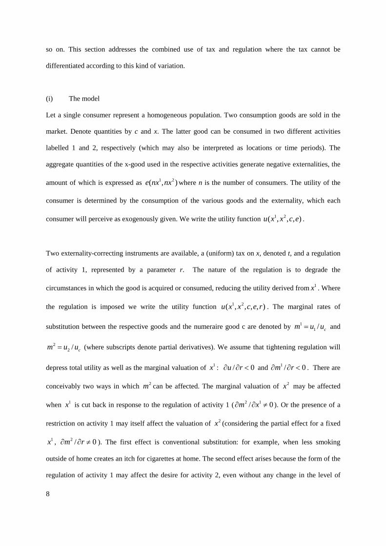
so on. This section addresses the combined use of tax and regulation where the tax cannot be

differentiated according to this kind of variation.

(i) The model

Let a single consumer represent a homogeneous population. Two consumption goods are sold in the

market. Denote quantities by c and x. The latter good can be consumed in two different activities

labelled 1 and 2, respectively (which may also be interpreted as locations or time periods). The

aggregate quantities of the x-good used in the respective activities generate negative externalities, the

amount of which is expressed as 1 2( , )e nx nx where n is the number of consumers. The utility of the

consumer is determined by the consumption of the various goods and the externality, which each

consumer will perceive as exogenously given. We write the utility function 1 2( , , , )u x x c e .

Two externality-correcting instruments are available, a (uniform) tax on x, denoted t, and a regulation

of activity 1, represented by a parameter r. The nature of the regulation is to degrade the

circumstances in which the good is acquired or consumed, reducing the utility derived from 1x . Where

the regulation is imposed we write the utility function 1 2( , , , , )u x x c e r . The marginal rates of

substitution between the respective goods and the numeraire good c are denoted by 11 / cm u u= and

22 / cm u u= (where subscripts denote partial derivatives). We assume that tightening regulation will

depress total utility as well as the marginal valuation of 1x : / 0u r∂ ∂ < and 1 / 0m r∂ ∂ < . There are

conceivably two ways in which 2m can be affected. The marginal valuation of 2x may be affected

when 1x is cut back in response to the regulation of activity 1 ( 2 1/ 0m x∂ ∂ ≠ ). Or the presence of a

restriction on activity 1 may itself affect the valuation of 2x (considering the partial effect for a fixed

1x , 2 / 0m r∂ ∂ ≠ ). The first effect is conventional substitution: for example, when less smoking

outside of home creates an itch for cigarettes at home. The second effect arises because the form of the

regulation of activity 1 may affect the desire for activity 2, even without any change in the level of

9

consumption in activity 1. The circumstances in which a given number of cigarettes are smoked

elsewhere (for example, standing outside, rather than in the relaxed environment of a bar or restaurant)

might conceivably induce an urge for smoking at home. Whether such an effect is likely to be

encountered obviously affects the complexity of our analysis of regulation. In most of the analysis we

rule out this possibility, and assume 2 / 0m r∂ ∂ = , but we revisit this issue later.

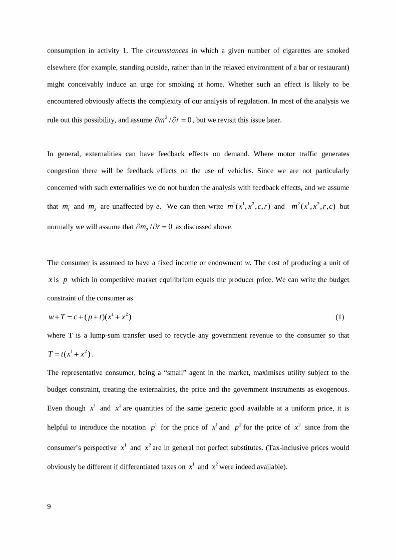
In general, externalities can have feedback effects on demand. Where motor traffic generates

congestion there will be feedback effects on the use of vehicles. Since we are not particularly

concerned with such externalities we do not burden the analysis with feedback effects, and we assume

that 1m and 2m are unaffected by e. We can then write 1 1 2( , , , )m x x c r and 2 1 2( , , , )m x x r c but

normally we will assume that 2 / 0m r∂ ∂ = as discussed above.

The consumer is assumed to have a fixed income or endowment w. The cost of producing a unit of

x is p which in competitive market equilibrium equals the producer price. We can write the budget

constraint of the consumer as

1 2( )( )w T c p t x x+ = + + + (1)

where T is a lump-sum transfer used to recycle any government revenue to the consumer so that

1 2( )T t x x= + .

The representative consumer, being a “small” agent in the market, maximises utility subject to the

budget constraint, treating the externalities, the price and the government instruments as exogenous.

Even though 1x and 2x are quantities of the same generic good available at a uniform price, it is

helpful to introduce the notation 1p for the price of 1x and 2p for the price of 2x since from the

consumer’s perspective 1x and 2x are in general not perfect substitutes. (Tax-inclusive prices would

obviously be different if differentiated taxes on 1x and 2x were indeed available).

10

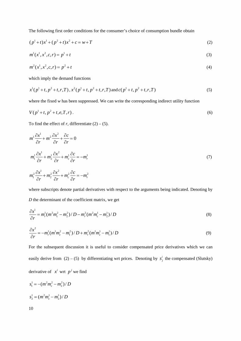
The following first order conditions for the consumer’s choice of consumption bundle obtain

1 1 2 2( ) ( )p t x p t x c w T+ + + + = + (2)

1 1 2 1( , , , )m x x c r p t= + (3)

2 1 2 2( , , , )m x x c r p t= + (4)

which imply the demand functions

1 1 2( , , , )x p t p t r T+ + , 2 1 2( , , , )x p t p t r T+ + and 1 2( , , , )c p t p t r T+ + (5)

where the fixed w has been suppressed. We can write the corresponding indirect utility function

1 2( , , , , )V p t p t e T r+ + . (6)

To find the effect of r, differentiate (2) – (5).

1 21 2 0x x cm m

r r r∂ ∂ ∂

+ + =∂ ∂ ∂

1 2

1 1 1 11 2 c r

x x cm m m mr r r

∂ ∂ ∂+ + = −

∂ ∂ ∂ (7)

1 22 2 2 21 2 c r

x x cm m m mr r r

∂ ∂ ∂+ + = −

∂ ∂ ∂

where subscripts denote partial derivatives with respect to the arguments being indicated. Denoting by

D the determinant of the coefficient matrix, we get

11 2 2 2 2 2 1 1

2 2( ) / ( ) /r c r cx m m m m D m m m m Dr

∂= − − −

∂ (8)

21 1 2 2 2 1 1 1

1 1( ) / ( ) /r c r cx m m m m D m m m m Dr

∂= − − + −

∂ (9)

For the subsequent discussion it is useful to consider compensated price derivatives which we can

easily derive from (2) – (5) by differentiating wrt prices. Denoting by ijs the compensated (Slutsky)

derivative of ix wrt jp we find

1 2 2 21 2( ) /cs m m m D= − −

1 2 1 12 2( ) /cs m m m D= −

11

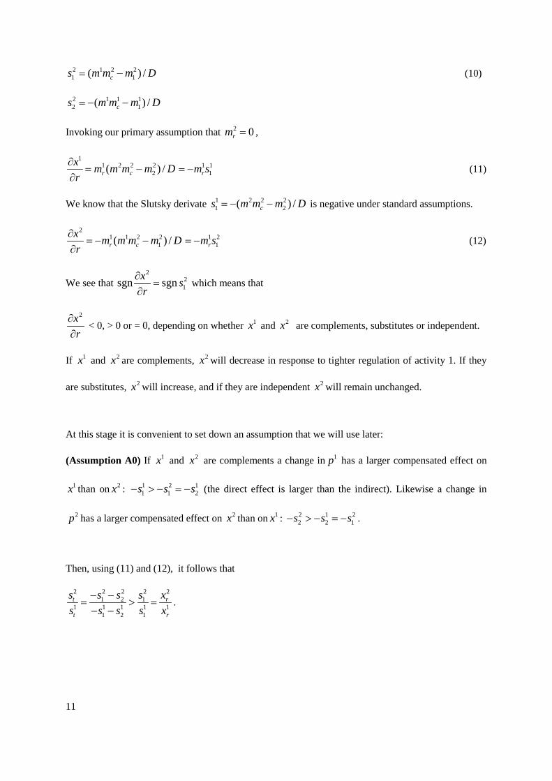
2 1 2 21 1( ) /cs m m m D= − (10)

2 1 1 12 1( ) /cs m m m D= − −

Invoking our primary assumption that 2 0rm = ,

11 2 2 2

2( ) /r cx m m m m Dr

∂= −

∂1 1

1rm s= − (11)

We know that the Slutsky derivate 1 2 2 21 2( ) /cs m m m D= − − is negative under standard assumptions.

21 1 2 2

1( ) /r cx m m m m Dr

∂= − −

∂1 2

1rm s= − (12)

We see that 2

21sgn sgnx s

r∂

=∂

which means that

2xr

∂∂

< 0, > 0 or = 0, depending on whether 1x and 2x are complements, substitutes or independent.

If 1x and 2x are complements, 2x will decrease in response to tighter regulation of activity 1. If they

are substitutes, 2x will increase, and if they are independent 2x will remain unchanged.

At this stage it is convenient to set down an assumption that we will use later:

(Assumption A0) If 1x and 2x are complements a change in 1p has a larger compensated effect on

1x than on 2x : 1 2 11 1 2s s s− > − = − (the direct effect is larger than the indirect). Likewise a change in

2p has a larger compensated effect on 2x than on 1x : 2 1 22 2 1s s s− > − = − .

Then, using (11) and (12), it follows that

2 2 2 2 21 2 1

1 1 1 1 11 2 1

t r

t r

s s s s xs s s s x

− −= > =− −

.

12

We conclude this discussion of the relationship between demands for the two goods and regulation by

re-visiting the case where regulation of activity 1 in itself affects the marginal valuation of activity 2,

so that 2 / 0m r∂ ∂ ≠ . Returning to (8) and (9) and using the equation system (10):

11 1 2 2 2 2 2 1 1

2 2( ) / ( ) /r r c r cxx m m m m D m m m m Dr

∂= = − − −∂

1 1 2 11 2r rm s m s= − + (13)

22 1 1 2 2 2 1 1 1

1 1( ) / ( ) /r r c r cxx m m m m D m m m m Dr

∂= = − − + −∂

1 2 2 21 2r rm s m s= − − (14)

We can ignore the possibility that 1 / 0x r∂ ∂ > since this would in any case be a counterproductive

regulation. Our main interest here is how 2x changes when 1x is regulated. When 1x and 2x are

substitutes, a regulation that discourages activity 1 will stimulate activity 2. Say, less smoking in

public places makes smoking at home more attractive. If the presence of the regulation itself has the

same effect ( 2 0rm > ) independent of any change in the amount consumed in activity 1 this will

reinforce the effect of the partial switching of consumption but it will not change the qualitative effects

of an analysis that allows for an increase in 2x .

When 1x and 2x are complements, regulation that discourages activity 1 will also discourage activity

2. Sticking to the smoking example, it may be that when smoking at work or in public places becomes

less pleasant and diminishes, the desire for nicotine in general subsides ( 2 0rm < ). This may not be an

implausible effect in the longer term. If the feeling of unpleasantness caused by the regulation

elsewhere also (for some psychological or other reason) carries over to smoking at home we would

once again have a reinforcing effect that would not change the qualitative effects of an analysis that

allows for a decrease in 2x . In a completely general analysis we cannot rule out the possibility that

regulation in and by itself might have effects that oppose those of substitutability or complementarity,

but we will not elaborate further on this in our analysis here.

(ii) Setting the tax and regulation

13

When both instruments are to be employed, how should they be used? It is useful to approach this

question in stages, firstly beginning with a partial analysis of the determination of the tax rate t for a

given regulation, secondly considering which consumption activity should be subject to regulation,

and thirdly, in (iii) below, considering the implications for the tax of tightening the regulation.

We start by formulating the Lagrange function

1 2 1 1 2 2 1 2

1 1 2 2 1 2

( , , ( ( , , , ), ( , , , ), )( ( , , , ) ( , , , ) )V p t p t e nx p t p t T r nx p t p t T r rtx p t p t T r tx p t p t T r Tµ

Λ = + + + + + +

+ + + + + + − (15)

where µ is the Lagrange multiplier assigned to the government’s budget constraint. To simplify

notation, let /V Tλ = ∂ ∂ , /eV V e= ∂ ∂ , / iie e x= ∂ ∂ . Differentiating with respect to t and making

use of the Slutsky decomposition, we get the first order conditions

1 2 1 1 2 21 1 1 2 2 1 2 2

1 1 2 1 1 2 2 21 1 2 2

/

/ / / /e e e e

e e e e

t x x V e s V e s V e s V e sV e x x T V e x x T V e x x T V e x x T

λ λ∂Λ ∂ = − − + + + +

− ∂ ∂ − ∂ ∂ − ∂ ∂ − ∂ ∂1 2 1 1 2 2

1 2 1 21 1 2 1 1 2 2 2/ / / / 0

x x ts ts ts tstx x T tx x T tx x T tx x T

µ µ µ µ µ µ

µ µ µ µ

+ + + + + +

− ∂ ∂ − ∂ ∂ − ∂ ∂ − ∂ ∂ = (16)

where ijs is the compensated derivative of ix with respect to jp .

1 21 2/ / /e eT V e x T V e x Tλ∂Λ ∂ = + ∂ ∂ + ∂ ∂ 1 1 2/ / 0t x T tx x Tµ µ µ+ ∂ ∂ + ∂ ∂ − = (17)

Multiplying (17) by and 1x and 2x , respectively, and making use of these new equations, we see that

(16) reduces to

( ) ( )1 1 2 21 1 2 2 1 2( ) ( ) 0e et V e s s t V e s sµ µ+ + + + + = (18)

Solving for t,

1 1 2 2 1 21 2 1 21 2 1 2

1 1 2 2 1 2 1 21 2 1 2

( ) ( )e e e et t

t t t t

V e V e V e V es s s s s st

s s s s s s s sµ µ µ µ

− − − −+ + +

= = ++ + + + +

(19)

14

where 1ts is the compensated (Slutsky) derivative of 1x with respect to t, and 2

ts is defined

analogously. Denoting the marginal social costs associated with 1x and 2x by 1ε and 2ε ,

respectively, i.e. e ii

V eεµ

−= , we can write t as the weighted average

1 21 2

1 1 2 21 2 1 2t t

t t t t

s st w ws s s sε ε ε ε= + = ++ +

. (20)

where 1w and 2w are the weights implicitly defined by the latter equation. (20) is of the same form as

the well-known weighted average formula of Diamond (1973) characterising the optimal uniform tax

rate on activities that generate non-uniform external costs in the absence of regulation. Thus we have

demonstrated that the weighted average formula for the tax holds also in this model where regulation

is also present, but we note that regulation will normally change the weights.

Turning to regulation and differentiating welfare with respect to the regulation parameter we find by

applying the Envelope Theorem to (15) .

1 2 1 21 21 2

1 2

/ / / / /

( ) / ( ) /e e r

r

r V e x r V e x r V t x r t x rt x r t x r V

µ µ

µ ε µ ε

∂Λ ∂ = ∂ ∂ + ∂ ∂ + + ∂ ∂ + ∂ ∂

= − ∂ ∂ + − ∂ ∂ + (21)

We are now in a position to show which of the consumption activities should be regulated:

Proposition 1

Subject to the assumptions 2 / 0m r∂ ∂ = and (A0), if a Pigouvian tax is to be supplemented by

regulation it is the consumption causing the larger marginal external cost that should be regulated.

Proof : Since rV is negative regulation will not be used unless (*) 1 11 2( ) ( ) 0r rt x t xε ε− + − > . When

1x and 2x are independent or substitutes so that 2 0rx > , (*) will only hold if 1 0t ε− < and activity 1

one has the larger marginal external cost. It is not worthwhile regulating activity one unless it has the

larger marginal external cost. Then consider the case when 1x and 2x are complements so that 2 0rx < .

15

From (A0) 2 2

1 1t r

t r

s xs x> . Then making use of

21

12

t

t

t st s

εε

−= −

−it follows that (**)

21

12

r

r

t xt x

εε

−< −

−. If

1 0t ε− < and 2 0t ε− > this is equivalent to 1 21 2( ) ( ) 0r rt x t xε ε− + − > and regulation may be

worthwhile. If 1 0t ε− > and 2 0t ε− < (**) is equivalent to 1 21 2( ) ( ) 0r rt x t xε ε− + − < and

regulation cannot be worthwhile.

Before discussing how the optimal tax should be adjusted in response to tighter regulation, we will

characterise the optimal level of regulation by equating the expression in (21) to zero. We can write

the ensuing optimality condition for regulation as

1 21 2( )( / ) ( ) / /rt x r t x r Vε ε µ− −∂ ∂ + − ∂ ∂ = − (22)

1 tε − shows how the tax falls short of the Pigouvian level. The term can be interpreted as the

uninternalised part of the external cost generated by 1x . We have previously found this term to have a

positive sign. 2t ε− is the (positive) excess tax on 2x , meaning taxation over and above the

Pigouvian level. It follows that we can interpret the former as a distortive subsidy and the latter as a

distortive tax. The whole left hand side is then the total alleviation of these distortions due to marginal

tightening of the regulation. This marginal gain should be equated to the maginal cost of regulation

caused by the disutility inflicted on the consumers. We may note that the former term on the left hand

side is positive, and the second term is also positive if the goods are substitutes, but will be negative

in the event that the goods are complements.

(iii) Implications of regulation for the externality tax

Recalling (20) we see that there are two ways in which the regulation can affect the optimal tax; it may

change the marginal external costs or alter the weights in the formula. There are no general results on

these changes, but still (20) provides a useful framework for considering how tighter regulation should

affect the externality tax.

16

Consider first the marginal external costs. When referring to this concept one usually has in mind an

individual’s marginal willingness to pay for a reduction in the externality level in terms of private

income, i.e. e iV eλ

−. However we could also consider e i

iV e λελ µ

−= which is measured in terms of

government revenue. The measures coincide in the event that the marginal cost of public funds

/ 1λ µ = . This will hold for optimal taxes if the utility function belongs to the class

1 2( , , ) ( , )u x x r v c r+ where e has been suppressed as we abstract from feedback effects from e3

iε

. In

that case we can think of as a standard marginal willingness to pay. Moreover, if we write the

utility function 1 2 1 2( , , ) ( , )c f x x r e nx nx+ − , which is quasi-linear in c, 1eV = − , 1λ = and 1µ =

(see appendix). Then the marginal external cost e ii

V e eλ

−= .

In order to narrow down the set of possible effects we will make a number of what we believe are

reasonable assumptions about marginal external costs.

(Assumption A1) We adopt the standard assumption in the externality literature that marginal external

costs are constant or increasing as the externality-generating activity expands. Expressing marginal

external costs in general as 1 21( , )x xε and 1 2

2 ( , )x xε 4

11 0

xε∂≥

∂

, standard assumptions will then imply that

and 22 0

xε∂

≥∂

. It will be observed that this assumption, while frequently made, is not

unrestrictive. It is not difficult to think of examples where the first unit of pollution causes the greatest

externality. The arrival of one smoker in a restaurant may cause greater marginal discomfort and

3 Where e enters multiplicatively or is additively separable the consumer’s choice is obviously invariant to the

value of e.

4 Alternatively, we might write the arguments as 1 2,nx nx and even include c, but n is fixed and can be

suppressed, and given 1 2,x x , c follows from the resource constraint.

17

annoyance to other diners than the marginal effect of the tenth smoker lighting up. We also assume

that cross effects are non-negative. 12 0

xε∂

≥∂

and 21 0

xε∂

≥∂

.

(Assumption A2) Our second assumption is that when one activity using x (activity 1) is being

regulated the total demand for x will diminish. This will obviously happen if 1x and 2x are

complements or independent. In the case of substitutes it will mean that the regulation of the use of 1x

induces some substitution towards 2x but not to the extent that the reduction in 1x is fully offset. Then

1 2

0x xr r

∂ ∂+ <

∂ ∂ and

2 1x xr r

∂ ∂< −

∂ ∂. Again, while this assumption may seem to cover many likely cases,

it is possible to think of examples where it would not hold. Supposing that a metropolitan area affected

by smog caused by motor vehicle NOx emissions were to restrict certain categories of motor vehicle

use in the most-heavily polluted downtown area. Drivers excluded from the central area might then

have to drive longer distances to get round the restricted area, and total NOx emissions could then rise.

(Assumption A3) A third assumption is that the marginal external cost of 1x is never more sensitive

to a change in 2x than to a change in 1x itself, i.e. 1 11 2x xε ε∂ ∂≥

∂ ∂. Analogously, 2 2

2 1x xε ε∂ ∂

≥∂ ∂

. We have

struggled to find plausible counterexamples to this assumption.

Considering the overall effect of r on the marginal external cost of 1x , 1 21( , )x xε , we have

1 21 1 1

1 2

x xr x r x rε ε ε∂ ∂ ∂ ∂ ∂= +

∂ ∂ ∂ ∂ ∂

Combining the assumptions above it follows immediately that 1 0rε∂≤

∂.

Now consider

1 22 2 2

1 2

x xr x r x rε ε ε∂ ∂ ∂ ∂ ∂

= +∂ ∂ ∂ ∂ ∂

18

If marginal costs are strictly increasing and 2x is non-increasing in r it follows that 2 0rε∂

≤∂

.

However, if 2x is increasing in r ( 1x and 2x are substitutes) and 22xε∂∂

is sufficiently large compared to

21xε∂∂

we may have 2 0rε∂

>∂

. Suppose for instance that regulation of driving at some time or in some

area induces substitution towards some other area or time where the marginal external cost then

increases as a result of larger traffic. However, we should note that substitution towards the other

activity does not necessarily imply this kind of result. Regulation of smoking in public places may

induce more smoking in private places, but if the externality generated in private places (say,

collectively-borne health costs) would alternatively be generated also in public places, there might be

no net effect on the marginal external cost. Assume quasi-linearity, 1 2 1 2( , ) ( , )u c f x x e nx nx= + − ,

and let 1 1 1 1 2( , ) ( ) ( ( ))e nx nx h nx s n x x= + + . Besides an externality generated by the total

consumption of the x-good (e.g. health effects) 1x generates a separate externality (e.g. smoking or

drinking which harms other people in public places). Then as discussed above 1eV = − , 1λ = , 1µ = ,

and 2 1 22 / '( ( ))e x ns n x xε = ∂ ∂ = + and 2 2

2 1x xε ε∂ ∂

=∂ ∂

. Then it follows, invoking (A2), that 2 0rε∂

≤∂

.

Let us sum up the partial effects of changes in marginal external costs, keeping weights constant. If at

least one marginal cost is increasing and 1x and 2x are independent or complements the optimal tax

will diminish in reponse to (tighter) regulation. If 1x and 2x are substitutes, the outcome is less clear-

cut. It is now conceivable, but, as we have seen, not necessary, that 2 0rε∂

>∂

. With 1 0rε∂

<∂

and

2 0rε∂

>∂

, the effect on t will depend both on the weights and on the relative changes in the marginal

external costs. It is possible that t will increase in response to (tighter) regulation if a large weight is

assigned to 2ε and this marginal external cost is steeply increasing.

19

Turning to the effects of regulation on the weights in (20) we see that if a smaller relative weight is

given to 1ε the partial effect is to lower t while the opposite case is conducive to a larger t. We notice

that the crucial question is how the price responsiveness of compensated demands is affected. We

should note that it is the relative price responsiveness that matters. In general little can be said about

how this property is affected. We can only look for special cases to give us a clue. Demand schedules

are often given a convex shape, i.e. they become flatter as the price declines and demand increases. If

the utility derived from a good x is separable from other goods we can write the good-specific utility

function as h(x) and the demand schedule is determined by '( )h x p= where p denotes the price. Then

we find / 1/ ''dx dp h= and 2 2 2/ '''/ ( '')d x dp h h= − . Invoking the analogy with the expected utility

function and the property of decreasing absolute risk aversion where h’’’<0 the convex shape obtains.

Going one step further, one may assume that a change in x due to regulation has the same effect as a

change due to a price increase so that demand becomes less price responsive as demand diminishes.

Assuming that the utility function belongs to the separable and quasi-linear class5

1 21 2( ) ( )h x h x c+ +

the arguments above might be invoked in our context. Now 1x and 2x would be

independent, a regulation would lower 1x and make it less price responsive without affecting the price

responsiveness of 2x . With increasing marginal external cost of 1x , t will diminish in response to

(tighter) regulation. This would lower the weight given to the external cost of 1x . When 1x and 2x are

substitutes 1x will decrease and 2x will increase owing to the regulation, and generalising the

reasoning above may suggest that the relative price responsiveness and the weight of 1x will diminish,

but we have to admit that the basis for this inference is weak. When 1x and 2x are complements the

regulation will diminish both and it appears less plausible that the weights will change, but again no

firm conclusion exists.

5 As discussed above there are many cases where the separability assumption does not seem appropriate.

20

The natural intuition is probably that a (stricter) regulation will lower t as the need for taxation may

appear less urgent when another instrument is being used (to a larger extent). Our discussion suggests

that this is indeed what will happen in many cases, but we have suggested two conceivable sources of

exceptions. First, where the two activities are substitutes, it is possible that t will increase in response

to (tighter) regulation if a large weight is assigned to 2ε and this marginal external cost is steeply

increasing. It is also possible that t will increase if the effect of tighter regulation is that demand for

1x becomes relatively more price responsive.

(iv) A ban on an activity.

It may not always be possible to find a way of implementing a “soft” regulation of the type above,

which selectively discourages a particular externality-generating activity by degrading the utility the

consumer derives from it. We may want to reduce the consumption of a good in a particular place to

alleviate the externality, for example, but this may be hard to enforce if the level of consumption

cannot be exactly monitored. In some circumstances, the only regulation that can be enforced may be a

ban, as the regulator will then only need to observe that somebody is consuming the good in order to

know that the regulation is being violated. We find, however, that regulation through a ban has very

different properties, when used in combination with imperfect externality taxation, than the soft

regulation discussed earlier. In particular, the rather unsurprising result in Proposition 1, that the

activity with the higher marginal external costs should be the one subject to regulation, turns out not to

hold when regulation can only take the form of a ban.

Banning an activity will have three effects, and a decision about whether to ban one or other activity

will depend on the net effect of these. Firstly, banning an activity will remove the external cost

previously caused by that activity. Secondly, it permits the external cost in the other activity to be fully

internalised as the tax on that activity will no longer be constrained by the concern with how it affects

the activity that has now been banned. Thirdly, it will deprive the consumer of the consumer surplus

(net of the external cost) in the activity that has been banned. If this final effect is large enough it could

21

outweigh the gains from the first two effects. Even if activity A causes a larger externality per unit

than activity B, what is relevant for a ban is in which activity the total external cost exceeds the total

consumer surplus. (We suppose that this does not happen in both activities, which would justify

banning the good altogether.) Thus even if a “soft” regulation will always be targeted at the activity

with the larger marginal external cost, this need not be the case with a ban (even if we imagine it will

often be the case).

A simple numerical example may suffice to illustrate the point. Consider the following separable

utility function 1 2 1 1 2 2 2 21 2( , , ) 0.5( ) 0.5( )u x x c c A x x A x x e= + − + − −

where 1 1 2 2 2 21 1 2 20.5 ( ) 0.5 ( )e D x E x D x E x= + + +

and i i

i

A p txB− −

=

We calculate the level of external costs and total utility, assuming the following parameter values

1 2 1 2 1 2 1 210, 5, 0.1, 0.1, 0.2, 0.4, 0.1, 0.2,A A B B D D E E= = = = = = = = p=2, w=100

If both the externality-generating activities are permitted, and a single tax is used to regulate them,

then tax should be set at t=2.92 and the total level of utility will be 340. The total external cost

generated by activity 1 will be 139.2 and the external cost generated by activity 2 will total 0.4. The

marginal external costs in the two activities will be 5.28 and 0.56 respectively. If the activity with the

higher marginal (and total) external cost (ie activity 1) is banned, then its external costs will not be

incurred, but consumer surplus will also be lost from this activity. The tax can be set on the remaining

activity 2 at 2t =2.13, and utility will be 211, lower than without the ban. If instead the activity

(activity 2) with lower external cost is banned, then the tax on the remaining activity can be set on at

1t =4.1, and utility will be higher, at 352. Thus we see that when regulation has to take the form of a

ban, rather than the discouragement of an activity through the "soft" regulation discussed earlier, the

superficially surprising result can be obtained that it could sometimes be more efficient to ban the less-

damaging activity.

22

III. Unwanted Differentiation – Tax Avoidance by Cross-border Shopping

Sometimes there may be cases in which uniform taxation is difficult to implement, even when

desirable, because the tax may be avoided in parts of the market. To fix ideas we shall consider a

regime where the domestic tax may be avoided by purchasing the good in question abroad, but the

example may be interpreted as representing more general cases. The important feature of the analysis

is that the tax can be avoided at a real resource cost. In this sense our analysis is akin to the literature

on risk-free but costly tax avoidance6

When there are countries with, respectively, inbound and outbound cross-border shopping, there may

be tax competition between the countries that may result in some equilibrium. (This is the approach

taken in Nielsen (2001)). We do not consider such competition but confine attention to the policy

choices of a single country taking conditions abroad as given, which would correspond to deriving the

response function of the country in a game situation leading to a Nash equilibrium. It suffices for our

purpose to have a country that is exposed to cross-border shopping in order to establish a costly tax

avoidance that will have implications for externality-correcting policies.

. While cross-border shopping is chosen as a specific example it

is also a case of major importance in many countries where consumers go abroad (or to other states in

the US) to buy goods many of which are supposed to generate externalities (alcohol, tobacco, petrol).

Suppose that an amount x of a good is purchased at home at a price p+t and an amount z is purchased

abroad at a retail price q and a (travel, etc.) cost k(z), where k’>0, k’’>0. The external cost depends

only on the aggregate consumption, and is given by the function e(nx+nz). The budget constraint is

( ) ( )w T c p t x qz k z+ = + + + + (23)

Where, as above, w is an exogenous income, and T is a lump-sum transfer used to return any

government revenue to the consumer and perceived as exogenous by the consumer. Hence, T=tx.

6 The idea is that by incurring a real resource cost, which is increasing in the amount of evasion/avoidance, a

share of the tax base can be sheltered from taxation. See for example Boadway et al. (1994).

23

As before, our notion of regulation is that it imposes a real cost of consuming the externality-

generating good. The utility function of a representative agent is

( , , , )u x z c e r+ (24)

where e=e(n(x+z)). Denoting partial derivatives by subscripts, we have 1 0x zu u u= = > ,

0cu > , 0eu < , 0ru < . Solving for c from the budget constraint and inserting into the utility function,

we have

( , ( ) ( ), , )u x z w T p t x qz k z e r+ + − + − − (25)

Maximising utility wrt x, z and c subject to the budget constraint treating the price, tax, income and the

externality as parametric, we obtain

1 ( ) 0cu u p t− + = (26)

1 ( '( )) 0cu u q k z− + = (27)

1 '( )c

u p t q k zu

= + = + (28)

Solving for z, we get 1' ( ) ( )z k p t q z p t−= + − = + after suppressing q. 1'

( ) ''( )z z

p t k z∂

= =∂ +

>0.

We may note that z is independent of the regulation, r. The regulation we consider is a regulation that

directly affects utility, such as restrictions on where, when, how, etc. alcohol, cigarettes, fuel can be

consumed. This will affect the total amount that is being purchased, but will not affect the amount that

is being purchased abroad since (at an interior optimum) this amount will be determined by the

marginal cost of cross-border shopping being equated to the domestic price which is taken as fixed.

Suppose that restrictions are imposed on smoking in certain places. This may induce people to smoke

less, but as long as people do not quit smoking, the part of the consumption that is more cheaply

acquired abroad will still be imported, and it is the residual domestic demand that is being adjusted in

response to regulation.

24

One may argue that cross-border shopping may be regulated7

, for instance this could happen by

regulating the allowances that can be imported duty-free. This would affect the cost of cross-border

shopping, k(z). This is a different kind of regulation from the one we address. The case we consider

will be valid for any given regulation of cross-border shopping as long as it is not prohibitively strict.

For instance within the EU it is quite lenient, and even outside the EU extensive cross-border

shopping takes place, even by people complying with the allowances. We simply take these

circumstances as given. We also recall that our key assumption is that tax avoidance is possible at a

cost, and other forms than cross-border shopping are conceivable.

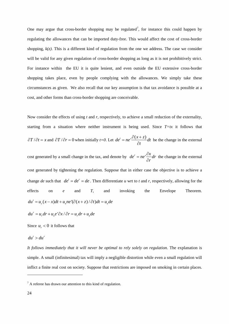
Now consider the effects of using t and r, respectively, to achieve a small reduction of the externality,

starting from a situation where neither instrument is being used. Since T=tx it follows that

/T t x∂ ∂ = and / 0T r∂ ∂ = when initially t=0. Let ( )'t x zde ne dt

t∂ +

=∂

be the change in the external

cost generated by a small change in the tax, and denote by 'r xde ne drr∂

=∂

the change in the external

cost generated by tightening the regulation. Suppose that in either case the objective is to achieve a

change de such that t rde de de= = . Then differentiate u wrt to t and r, respectively, allowing for the

effects on e and T, and invoking the Envelope Theorem.

( ) '( ( ) / )tc e edu u x x dt u ne x z t dt u de= − + ∂ + ∂ =

' /rr e r edu u dr u e x r u dr u de= + ∂ ∂ = +

Since 0ru < it follows that

t rdu du>

It follows immediately that it will never be optimal to rely solely on regulation. The explanation is

simple. A small (infinitesimal) tax will imply a negligible distortion while even a small regulation will

inflict a finite real cost on society. Suppose that restrictions are imposed on smoking in certain places.

7 A referee has drawn our attention to this kind of regulation.

25

Where restrictions apply to few places the the disbenefit may be small, but there is no reason why it

should be zero. Even slightly degrading the circumstances in which the units of the good are

consumed will make the consumer worse off. This is different from a tax which does not in and by

itself diminish utility but only works through changes in the consumption bundle.

A further implication is that at a very low level of government intervention, the externality-alleviating

policy will rely solely on taxation. Indeed this would be the case where the externality itself is minor.

Proposition 2

Where a tax and a costly regulation may coexist it will never be optimal to rely solely on regulation.

At a sufficiently modest level of intervention the tax is the only instrument deployed at the optimum.

A conceivable caveat is that the introduction of a tax may involve an administrative cost so that a

“small” tax is not costless. Such a cost might deprive the tax of its edge over regulation but only if

adopting the regulation is less costly in terms of administration.

Consider now the case where initially the tax is the only instrument in use. We may then ask how

introducing regulation will affect the tax-setting. The first order condition for the optimal use of t is

derived by differentiating the utility function, taking into account that T=tx and invoking the Envelope

Theorem.

( ) 0( )c e

u x e x zu x x t u nt t x z t

∂ ∂ ∂ ∂ + = − + + + = ∂ ∂ ∂ + ∂ (29)

A slight reformulation yields

( ) ( )' 0ec

c

u x z z u x zu t t net t t u t

∂ ∂ + ∂ ∂ + = − + = ∂ ∂ ∂ ∂ (30)

The corresponding second order condition is

26

2

2 0ut

∂<

∂ (31)

The first order condition implies that

( )'e

c

u x z zne t tu t t

− ∂ + ∂ − − = − ∂ ∂ (32)

'e

c

u neu−

is the consumer’s marginal willingness to pay for escaping the external cost of a marginal unit

of the good. We can then interpret 'e

c

u ne tu−

− as the uniternalised part of the externality caused by a

marginal unit, which is strictly positive when t>0. From the first order conditions for the consumer

'( )t q k z p= + − , which means that t reflects the excess social cost of buying the good abroad rather

than domestically. It measures the real resources used up by the consumer in order to pursue a tax

saving by doing cross border shopping. So the condition states a trade-off between the cost of cross-

border shopping induced by a larger tax and the gain achieved in terms of lower external costs.

We may then ask how introducing regulation will affect the tax-setting. Departing from the first order

condition we can use standard comparative statics to explore the effect on the tax.

2

2

( )' ' 0e ec c

c c

u t u x x z uu t e u net r u r t t r u

∂ ∂ ∂ ∂ ∂ + ∂ −+ + − = ∂ ∂ ∂ ∂ ∂ ∂

12

2

( )' ' 0e ec c

c c

t u x x z u uu ne t u ner u r t t r u t

− ∂ − ∂ ∂ ∂ + ∂ − ∂ = − − − − = ∂ ∂ ∂ ∂ ∂ ∂ (33)

Obviously 12

2

ut

− ∂− ∂

is positive from the second order condition. Moreover , it follows from the first

order condition that a change in r will have two effects both of which appear on the right hand side of

(33). As stated above, we can interpret 'e

c

u ne tu−

− as the uninternalised part of the externality caused

by a marginal unit of the good, which is positive. The price responsiveness of the demand, xt

−∂∂

, will

27

then determine how efficient the tax is in realising the social gain from further reduction of

consumption. A crucial question is how regulation will affect the price resoponsiveness. If regulation

increases the price responsivenss and makes the tax a more efficient instrument this is cet. par.

conducive to a larger tax. In the previous section we suggested that lower demand is often assumed to

imply less price responsive demand, even though there is not a very firm basis for this claim. If true,

the partial effect will be a lowering of the tax.

The second term ( ) 'e

cc

x z uu net r u

∂ + ∂ −− ∂ ∂

has the sign of ' 'e e

c c

u une ner u u ∂ − − ∂

which we assume is

negative (or conceivably zero). When the marginal external cost curve is increasing the term is

negative, and tighter regulation will diminish the externality and lower the marginal external cost

implying that there is less need for the externality tax. We sum up in the following.

Proposition 3

Let the tax be the only instrument optimally in use. Then introducing a marginal regulation has the

following partial effects:

a) lower (higher) tax if regulation makes domestic demand less (more) sensitive to a tax increase,

b) lower tax if the marginal external cost is increasing in consumption.

Where t is ”large” any change in t will take place from a distorted point of departure and there is

conceivably a sizeable marginal cost associated with using the tax alone to mitigate the externality.

The tax imperfection due to partial enforcement implies that it is not only the regulation that entails a

real cost. We note that where the tax (and price) response of cross-border shopping is (close to)

constant the right hand side of (32) is obviously increasing in t. If the demand schedule becomes

steeper as demand declines with increasing price this effect is being reinforced. Unless the marginal

cost of regulation is overly large, gradually increasing the tax will take us to a point where the

28

marginal cost of taxation no longer falls short of the marginal cost of regulation, and efficiency

requires that the regulation kicks in.

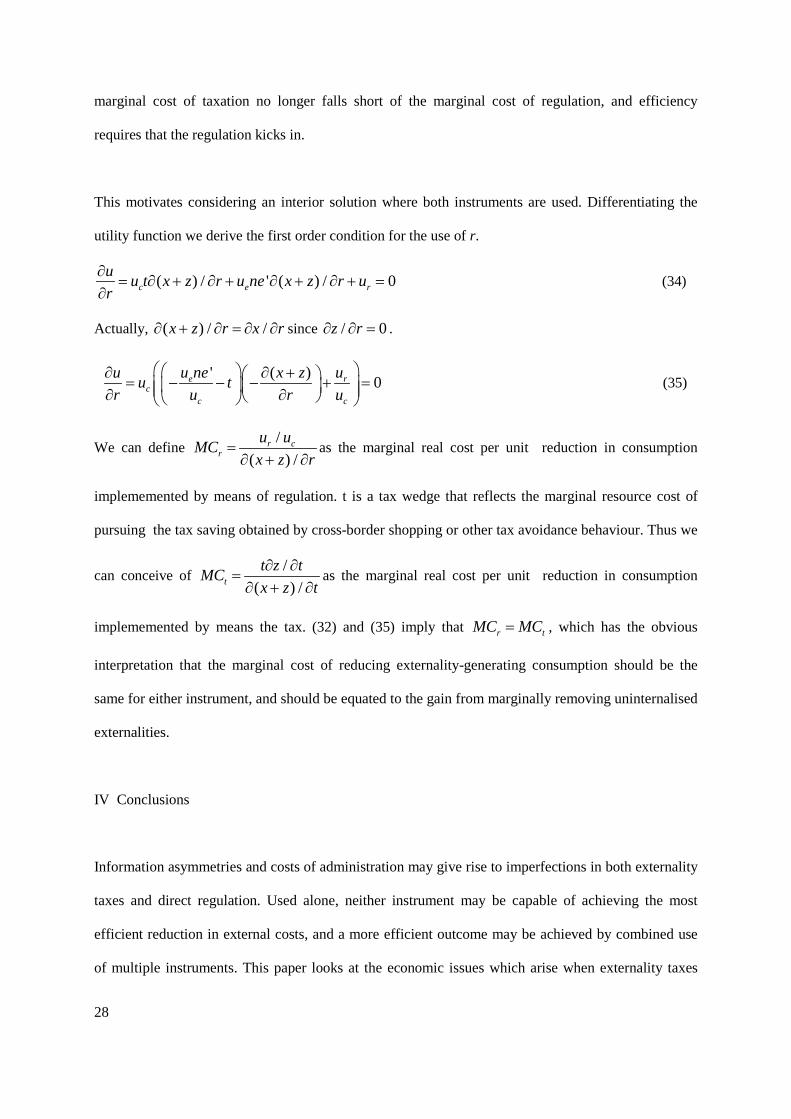
This motivates considering an interior solution where both instruments are used. Differentiating the

utility function we derive the first order condition for the use of r.

( ) / ' ( ) / 0c e ru u t x z r u ne x z r ur∂

= ∂ + ∂ + ∂ + ∂ + =∂

(34)

Actually, ( ) / /x z r x r∂ + ∂ = ∂ ∂ since / 0z r∂ ∂ = .

' ( ) 0e r

cc c

u u ne x z uu tr u r u

∂ ∂ + = − − − + = ∂ ∂ (35)

We can define /

( ) /r c

ru uMCx z r

=∂ + ∂

as the marginal real cost per unit reduction in consumption

implememented by means of regulation. t is a tax wedge that reflects the marginal resource cost of

pursuing the tax saving obtained by cross-border shopping or other tax avoidance behaviour. Thus we

can conceive of /

( ) /tt z tMCx z t∂ ∂

=∂ + ∂

as the marginal real cost per unit reduction in consumption

implememented by means the tax. (32) and (35) imply that r tMC MC= , which has the obvious

interpretation that the marginal cost of reducing externality-generating consumption should be the

same for either instrument, and should be equated to the gain from marginally removing uninternalised

externalities.

IV Conclusions

Information asymmetries and costs of administration may give rise to imperfections in both externality

taxes and direct regulation. Used alone, neither instrument may be capable of achieving the most

efficient reduction in external costs, and a more efficient outcome may be achieved by combined use

of multiple instruments. This paper looks at the economic issues which arise when externality taxes

29

and direct regulation are used in parallel. It explores the properties of two simple models of imperfect

tax and imperfect regulation, reflecting different form of imperfection in the tax instrument.

The focus of the paper is on externalities arising from individuals’ consumption decisions. A number

of such externalities are affected by the kinds of instrument inefficiency we describe. Taxes on the sale

of alcoholic drinks or tobacco products, for example, can only roughly approximate the externalities

generated by their consumption. Likewise the available forms of regulation, such as the recent ban on

smoking in public places in many European countries, are not precisely targeted to the underlying

external costs.

Regulation may affect consumption behaviour in a number of ways. We suggest that for a number of

consumer externalities it may be useful to think of regulation as an increase in the cost to consumers of

obtaining the good (for example, where the sale of alcoholic drinks is limited to a small number of

outlets). Regulation thus has effects which are similar to - but not equivalent to - an increase in price.

It will be seen that the representation of regulation here differs sharply from the emission limits or

technology mandates typically considered when analysing the regulation of industrial emissions.

Section 2 considered a case where an externality tax cannot be adequately differentiated to reflect

differences in the external costs from different units consumed. Costs may differ between individuals,

or between consumption in different contexts, and yet the tax is constrained to be uniform. We show

that in this situation the outcome can be improved by direct regulation of consumption generating the

larger external cost. The optimal externality tax rate in this context takes the same form as the well-

known weighted average formula of Diamond (1973). How it is affected by the addition of regulation

will depend on how marginal external costs and the price responsiveness of demand vary with

consumption. Where these are constant, tighter regulation has no effect on the optimal tax, but if the

marginal external cost is increasing in consumption and the price responsiveness is affected the

optimal tax may change. While in several circumstances we find support for the intution that there is

30

less need for the tax when another instrument is introduced to curb externalities, there are possible

exceptions. The regulation may conceivably increase the tax if aggregate marginal external costs

increase because substitution towards the unregulated consumption drives up its marginal external cost

substantially or regulation raises the relative weight of the more serious externality.

Section 3 considered a contrasting case where the tax exhibits undesirable differentiation - for example

where some consumption escapes the externality tax, by being purchased in lower-price countries

abroad or on the black market. Where this happens, an externality-motivated commodity tax will

distort the choice between different sources of supply and the resulting excess burden will be

increasing in the tax rate. We show that the optimal policy mix will depend on the scale of

intervention required. Where there is a major externality it will, as before, be optimal to deploy both

instruments, set at a level to equate the marginal cost per unit reduction in consumption from each

instrument. However, although both instruments are imperfect, combined use will not always be

optimal. We demonstrate that in cases where the externality is small, it will be efficient to control

externality effects using the tax alone, and it will never be optimal to rely solely on regulation. The

intuition for this result is straightforward: regulation always inflicts a finite real resource cost on

society, while a small (infinitesimal) tax involves negligible distortion.

We then consider the implications of introducing regulation, starting from a situation where the

externality is controlled through the use of a tax alone. The optimal tax rate will diminish if regulation

and the resulting fall in externality-generating consumption lower the marginal external cost and

weakens the price responsiveness of demand. The former effect reduces the need for the tax and the

latter reduces the efficiency of the tax instruments. It follows that the opposite effect is conceivable if

regualtion makes demand more price responsicve and the tax instrument more efficient.

Our models have in common that using the tax to internalise an externality is costly because it it is

distortionary in some other respect. In the former model, increasing the tax to alleviate the more

31

serious externality will over-internalise the weaker externality. In the latter model a larger tax will

better internalise the externality but will increase the locational distortion. We note that in both models

sensitivity of demand is crucial to the effect of tighter regulation on the optimal externality tax In the

first model the tax is a more (less) efficient instrument for diminishing the externality where the

demand causing the more serious externality becomes more (less) price sensitive in response to the

regulation. In the second model more price responsive domestic demand makes the tax a more

efficient instrument for diminishing the quantity consumed and the associated externality. With larger

sensitivity the externality can be depressed more without creating a larger tax wedge between sources

of supply.

Appendix

It follows from (17) that

1 2 1 21 2/ / 1 / /e eV Ve x T e x T t x T t x Tλ

µ µ µ+ ∂ ∂ + ∂ ∂ = − ∂ ∂ − ∂ ∂ (a1)

We easily see that 1λµ= is equivalent to

1 2 1 21 2/ / / /e eV Vt x T t x T e x T e x T

µ µ− −

∂ ∂ + ∂ ∂ = ∂ ∂ + ∂ ∂ (a2)

This equation obviously holds if 1 2/ / 0x T x T∂ ∂ = ∂ ∂ = which would imply a quasi-linear utility

function which is linear in c since only c will vary with income. If not, (a2) is equivalent to

1 2

1 21 2 1 2

/ // / / /

e eV x T V x Tt e ex T x T x T x Tµ µ

− ∂ ∂ − ∂ ∂= +

∂ ∂ + ∂ ∂ ∂ ∂ + ∂ ∂ (a3)

Since at the optimum t will satisfy (19)

1 21 2

1 1 1 1

e et t

t t t t

V e V es st

s s s sµ µ

− −

= ++ +

(a3) will hold if

1 2 1 2

// /

i it

t t

s x Ts s x T x T

∂ ∂=

+ ∂ ∂ + ∂ ∂ for i=1,2 (a4)

32

We can show that this will hold if the utility function can be written as 1 2( , ) ( )u x x v c+ , where e has

been suppressed since we abstract from feedback effects from e. Substituting from the budget

constraint we can rewrite the utility function as

1 2 1 2( , ) ( ( ) ( ) )u x x v w T p t x p t x+ + − + − + (a5)

The optimality conditions for the consumer’s choice of 1x and 2x are then

1 2 1 21( , ) '( ( ) ( ) ) 0u x x qv w T p t x p t x− + − + − + = (a6)

1 2 1 22 ( , ) '( ( ) ( ) ) 0u x x qv w T p t x p t x− + − + − + = (a7)

were q=p+t and subscripts denote partial derivatives.

Second order conditions are

211 ''u q v+ <0 (a8)

2 211 12

2 221 22

'' ''det 0

'' ''u q v u q v

Du q v u q v + +

= > + +

(a9)

where ’det’ denotes the determinant of the matrix.

Now consider a compensated change in t. We can think of the compensation as being given by an

increase in T, 1 2/dT dt x x= + , which keeps c unchanged for fixed values of 1x and 2x . Denote by

its the compensated derivative of ix with respect to t (i=1,2). Differentiating we find

(a10)

(a11)

(a12)

211 12

1 '( )ts v u uD

= − (a13)

1 211 12 22

1 '( 2 )t ts s v u u uD

+ = − + (a14)

2 1 2 211 12( '') ( '') ' 0t tu q v s u q v s v+ + + − =

2 1 2 221 22( '') ( '') ' 0t tu q v s u q v s v+ + + − =

122 12

1 '( )ts v u uD

= −

33

2 1 2 211 12( '') ( '') '' 0T Tu q v x u q v x qv+ + + − = (a15)

2 1 2 221 22( '') ( '') '' 0T Tu q v x u q v x qv+ + + − = (a16)

Now consider the effects of changing T where /i iTx x T= ∂ ∂ (i=1,2).

122 12

1 ''( )Tx qv u uD

= − (a17)

211 12

1 ''( )Tx qv u uD

= − (a18)

1 222 12 11

1 ''( 2 )T Tx x qv u u uD

+ = − + (a19)

We immediately realise that 1 2 1 2

i it T

t t T T

s xs s x x

=+ +

( i=1,2) and (a4) is satisfied

References

Atkinson, A. B. and Stiglitz J. E. (1976), The Design of Tax Structure: Direct versus Indirect

Taxation, Journal of Public Economics 6, 55-75.

Balcer, Y., (1980), Taxation of Externalities: Direct versus Indirect, Journal of Public Economics 13,

121-129.

Boadway, R., Marchand M. and Pestieau, P. (1994), Towards a Theory of the Direct-Indirect Tax

Mix, Journal of Public Economics 55, 71-88.

Bovenberg, A.L. and Goulder, L.H., (2002), Environmental Taxation and Regulation, in A. J.

Auerbach and M. Feldstein (eds.), Handbook of Public Economics, Elsevier, New York,

1471-1545.

Christiansen, V. (1984), Which Commodity Taxes Should Supplement the Income Tax? Journal of

Public Economic 24, 195-220.

Christiansen V. and S. Smith (2009), Imperfect Externality-Correcting Taxes and Regulation when

Revenues Matter. Mimeo.

Cnossen, S. (2005), Theory and Practice of Excise Taxation. Smoking, Drinking, Gambling, Polluting,

34

and Driving, Oxford University Press, Oxford.

Corlett, W. J. and Hague, D. C. (1953), Complementarity and the Excess Burden of Taxation, Review

of Economic Studies 21, 21–30.

Crawford, I., Keen, M. and Smith, S. (2009), “Value Added Tax and Excises” in Institute for Fiscal

Studies (ed) Dimensions of Tax Design. Background papers for the Mirrlees Review of the UK Tax

System, Oxford University Press, Oxford.

Diamond, P.A. (1973), Consumption Externalities with Imperfect Corrective Pricing, Bell Journal of

Economics 4, 526-38.

Eskeland, G.S. (1994), A Presumptive Pigouvian Tax: Complementing Regulation to Mimic an

Emissions Fee, World Bank Economic Review 8, 373-94.

Fullerton, D. and Wolverton, A. (1999), The Case for a Two-part instrument: Presumptive Tax and

Environmental Subsidy, in A Panagariya, P.R. Portney and R. M. Schwab (eds), Environmental and

Public Economics. Essays in Honor of Wallace E. Oates, Edward Elgar, Cheltenham.

Green, J. and Sheshinski, E. (1976), Direct versus Indirect Remedies for Externalities. Journal of

Political Economy 84, 797-808.

Hoel, M., (1998), Emission Taxes versus Other Environmental Policies, Scandinavian Journal of

Economics 100, 79-104.

Hoel, M. (1997), International Coordination of Environmental Taxes, in C. Carraro and D. Siniscalco

(eds.), New Directions in the Economic Theory of the Environment, Cambridge University Press,

Cambridge,105-146.

Innes, R. (1996), Regulating Automobile Pollution under Certainty, Competition and Imperfect

Information. Journal of Environmental Economics and Management 31, 219-239.

Mandell, S. (2004), Optimal Mix of Price and Quantity Regulation under Uncertainty. Stockholm

University Research Papers in Economics, 204:12

Mendelsohn, R. (1986). “Regulating Heterogeneous Emissions,” Journal of Environmental Economics

and Management 13(4); 301-312.

35

Montero, J-P. (2005). “Pollution Markets with Imperfectly-Observed Emissions,” RAND Journal of

Economics 36; 645-660.

Montgomery, D.W. (1972). “Markets in Licenses and Efficient Pollution Control Programs,” Journal

of Economic Theory 5; 395-418..

Pirttilä, J. and Tuomala M. (1997), Income Tax, Commodity Tax and Environmental Policy

International Tax and Public Finance 4, 379-393

Roberts, M. J. and Spence, M. (1976), Effluent Charges and Licenses under Uncertainty", Journal of

Public Economics 5, 193-208.

Sandmo, A., (1976), Direct versus Indirect Pigovian Taxation. European Economic Review 7, 337-

349.

Sandmo, A., (2000), The Public Economics of the Environment, Oxford University Press, Oxford.

Weitzman, M. L. (1991), Prices vs. Quantities, Review of Economic Studies 41, 477-91.

Wijkander, H., (1985), Correcting Externalities through Taxes on Subsidies to Related Goods, Journal

of Public Economics 28, 111-125.