1989 A New Technique for Fully Efficient 3Dkmlee.gatech.edu/me6406/handeye.pdf · A New Technique for Fully Autonomous and Efficient 3D Robotics Hand/Eye Calibration ... and equal

IEEE TRANSACTIONS ON ROBOTICS AND AUTOMATION, VOL. 5, NO. 3, JUNE 1989 345

A New Technique for Fully Autonomous and Efficient 3D Robotics Hand/Eye Calibration

ROGER Y. TSAI AND REIMAR K. LENZ

Abstract-This paper describes a new technique for computing 3D position and orientation of a camera relative to the last joint of a robot manipulator in an eye-on-hand configuration. This is part of a trio for real-time 3D robotics eye, eye-to-hand, and hand calibrations, which use a common setup and calibration object, common coordinate systems, matrices, vectors, symbols, and operations throughout the trio, and is especially suited to machine vision community. It is easier and faster than any of the existing techniques, and is ten times more accurate in rotation than any existing technique using standard resolution cameras, and equal to the state-of-the-art vision based technique in terms of linear accuracy. The robot makes a series of automatically planned movements with a camera rigidly mounted at the gripper. At the end of each move, it takes a total of 90 ms to grab an image, extract image feature coordinates, and perform camera extrinsic calibration. After the robot finishes all the movements, it takes only a few milliseconds to do the calibration. A series of generic geometric properties or lemmas are presented, leading to the derivation of the final algorithms, which are aimed at simplicity, efficiency, and accuracy while giving ample geometric and algebraic in- sights. Besides describing the new technique, critical factors influencing the accuracy are analyzed, and procedures for improving accuracy are introduced. Test results of both simulation and real experiments on an IBM Cartesian robot are reported and analyzed.

I. INTRODUCTION

A . The Calibration Trio

N ORDER for a robot to use a video camera to estimate the I 3D position and orientation of a part or object relative to its own base within the work volume, it is necessary to know the relative position and orientation between the hand and the robot base, between the camera and the hand, and between the object and the camera. These three tasks require the calibration of robot, robot eye-to-hand, and camera (see Fig. 1). These three tasks normally require large-scale nonlinear optimization, special setup, and expert skills. We have developed three techniques to deal with these three tasks. They are as follows:

1) Camera Calibration (see [6], [ 101, [ 1 11, [ 131). 2) Robot Eye-to-Hand Calibration (this paper). 3) Cartesian Robot Hand Calibration [ 5 ] .

Manuscript received December 16, 1987; revised December 6, 1988. Part of the material in this paper was presented at the 4th Int. Symp. on Robotics Research, Santa Cruz, CA, Aug. 9-14, 1987.

R. Y. Tsai is with IBM Thomas J. Watson Research Center, Yorktown Heights, NY 10598.

R. K. Lenz was with the IBM Thomas J. Watson Research Center, York- town Height, NY 10598. He is now with Lehrstuhl f i r Nachrichtentechnik, Technische UniversiCt Munchen, D-8000, Munchen 2, West Germany.

IEEE Log Number 8927074.

CAUB ATlON ‘1 CALIBRATIO

Fig. 1. To obtain the 3D position and orientation of an object relative to the robot world base, it is necessary to perform three calibrations; namely, robot hand, eye-to-hand, and eye (camera) calibration.

The advantages of the techniques are as follows: 1) They are faster than any other vision-based calibration

technique by at least an order of magnitude. The camera calibration takes only 25 ms on a 68000-based

minicomputer plus 65 ms to read the image into the computer and extract the image feature coordinates (centers of 36 circular discs) with better than 1-pm accuracy in the image space. For the other two calibrations, the robot makes a series of moves, and at the end of each move, a camera calibration is performed. At the end of all the moves, a few milliseconds are needed to finalize the calibration trio.

2) The techniques are at least as accurate as any existing technique using vision.

3) The three calibrations share the following: setup, calibration plate, image feature extraction procedure, definition of symbols and matrix representations, robot motion, and processing equipment.

4) The calibration need not be 3D. It can be coplanar. This makes the construction of high-accuracy target points possible (see the next section for the description of targets).

5) They are friendly to machine vision people and do not require special skills.

This paper describes the second calibration procedure.

B. 3 0 Robotics Hand/Eye Calibration 3D robotics hand/eye calibration is the task of computing

the relative 3D position and orientation between the camera and the robot gripper in an eye-on-hand configuration, mean- ing that the camera is rigidly connected to the robot gripper. The camera is either grasped by the gripper, or just fastened to it. More specifically, this is the task of computing the rel-

* When doing feature extraction, off-the-shelf general-purpose image processing hardware boards were used for frame grabbing, thresholding, and boundary location estimation.

1042-296X/89/0600-0345$01 .OO O 1989 IEEE

Authorized licensed use limited to: Georgia Institute of Technology. Downloaded on October 16, 2008 at 10:06 from IEEE Xplore. Restrictions apply.

346 IEEE TRANSACTIONS ON ROBOTICS AND AUTOMATION, VOL. 5 , NO. 3, JUNE 1989

ative rotation and translation (homogeneous transformation) between two coordinate frames, one centered at the camera lens center, and the other at the robot gripper. The gripper coordinate frame is centered on the last link of the robot manipulator, and as we shall see in this paper, the robot manipulator must possess enough degrees of freedom so as to be able to rotate the camera around two different axes while at the same time keeping the camera focused on a station- ary calibration object in order to resolve uniquely the full 3D geometric relationship between the camera and the gripper .2

C. The Difficulties of the Problem It is obvious that if the robot knows the exact 3D posi-

tions of a number of points on a calibration setup in the robot world coordinate system as well as the 3D location of the gripper, while at the same time, the camera can view these points in a proper way, then it is possible to determine the 3D homogeneous transformation between the camera and the calibration world coordinate frame, making it a trivial matter to compute the homogeneous transformation between the camera and the manipulator. However, it is very difficult, if at all possible, for the robot to acquire accurate knowledge of the 3D positions of a number of feature points easy enough for the camera to view simultaneously with the right resolution, field of view, etc., while the position information has to be known in the robot world coordinate system. Some re- searchers treat the difference between the calibration world coordinate system and the robot world coordinate system as a 6-degree-of-freedom unknown, and incorporate them into a much larger nonlinear optimization process (see “The Rea- sons why the State-of-the-Art Is Deficient” later in the paper). We propose a much easier and faster approach.

D. The Importance of 3 0 Hand/Eye Calibration The calibration is important in several aspects: Automated 3D Robotics Vision Measurement: When vi-

sion is used to measure 3D geometric relationships between different parts of an object in a robotics work cell, it is often necessary to use the manipulator to move the vision sensor to different positions in the work space in order to see different features of the object (see [15]). At each point, the 3D position and orientation of the feature measured by the vision system is only relative to the vision sensor. As the manipulator moves the sensor to different positions, the measurements taken at different positions are not related to one another unless we know the 3D relative position and orientation of the sensor at different locations. If the robot system is capable of knowing where the gripper is in the robot world coordinate system to some degree of accuracy, then it should know how much 3D motion it has undertaken from one position to another. Since the camera is rigidly connected to the gripper, of course it also undergoes the same rigid body motion, but only in the robot world coordinate system. If the hand/eye calibration is not done, one does not know the 3D homogenous transformation between the camera 3D coordinate systems at different locations simply from the motion of the robot manipulator.

*It takes at least two rotary joints and one linear joint, or three rotary joints. It is possible to use just two rotary joints, but the rotation axes for these two joints must coincide at the calibration block.

Automated Sensor Placement Planning: In order to do automated 3D measurement with robot vision, sensor planning is vital in order to automatically determine the optimum positions of the sensor so that all the desired features can be viewed while taking care of problems of occlusion, depth of focus, resolution, field of view, etc. However, even if the robot knows where to put the sensor for optimum viewing, it does not know where the manipulator should be in order to achieve this goal, unless the 3D geometric relationships between the last link of the manipulator and the sensor are known.

Automated Part Acquisition or Assembly: When vision is used to aid the robot in grasping an object for automated assembly or part transport with eye-on-hand configuration, unless iterative visual feedback is used, the vision system may be able to determine where the part is relative to the sensor, but the robot does not know how to place the manipulator to grasp it. This problem can be resolved by performing robot handleye calibration.

Stereo Vision: If only one camera is used to do stereo vision, one way to create a stereo base is to move the camera with the manip~lator.~ Although the robot system may know how much the manipulator has moved, it does not know the homogeneous transformation between the 3D camera coordinate system, even if the camera undergoes the same rigid body motion as the gripper does (since the rigid body motion is defined only in the robot world coordinate system). Again, when the hand/eye calibration is performed, this problem is solved.

E. The Reasons why the State-of-the-Art is Deficient From our literature survey, there are two categories of ap-

proaches for doing robot hand/eye calibration: Coupling Hand/Eye Calibration with Conventional

Robot Kinematic Model Calibration: References (partial list): [l], [3], [7]. In this approach, global nonlinear optimization is done over the robot kinematic model parameters an the hand/eye parameters simultaneously, making the number of unknowns generally over 30. Such large-scale nonlinear optimization is very time-consuming, and needs a very good initial guess and accurate data for convergence. It also cannot easily exploit the use of redundant images and stations for re- ducing error since the computation would become prohibitive.

Decoupling Hand/Eye Calibration from Conventional Robot Kinematic Model Calibration: References (partial list): [9], [12], this paper. As far as we know, Shiu and Ah- mad’s work [9] and the work reported in Tsai and Lenz [12] as well as this paper are the first attempts to decouple the hand/eye calibration from robot model calibration and not use global high-dimensional nonlinear optimization. The starting point in these two works are similar (although independently developed), the solutions are very different. In Shiu and Ah- mad’s method, the number of unknowns to solve for is twice the number of degrees of freedom, since they treat sin and cos functions as independent. We found it advantageous to use

This is not highly recommendable except in low accuracy applications. It is better for the robot to carry a stereo pair of cameras or a laser-camera pair, or to use one camera with model-based location determination.


TSAI AND LENZ: FULLY AUTONOMOUS AND EFFICIENT 3D ROBOTICS HAND E Y E CALIBRATION 347

WORLD

Fig. 2. Basic setup for robot hand/eye calibration. Ci and Gi are coordinate frames for the camera and gripper, respectively.

Fig. 4. The physical setup. A CCD camera is rigidly mounted on the last joint of an IBM Clean Room Robot for performing hand/eye calibration.

Fig. 3. The physical setup. A CCD camera is rigidly mounted on the last joint of an IBM Clean Room Robot for performing hand/eye calibration.

redundant frames to improve accuracy, but in our algorithm, the number of unknowns stays the same no matter how many frames are used simultaneously, and for each additional frame, only 60 additional arithmetic scalar operations are needed (each operation takes less than half a microsecond on a typical minicomputer). In Shiu and Ahmad’s method, the number of unknowns increases by two for each extra frame. Our procedure is simpler and faster, and the derivation procedure is also simpler. We have also done extensive error analysis, simulation and real experiments for testing the accuracy potential or problems of hand/eye calibration, and propose means for improving accuracy.

11. THE NEW APPROACH

A . Basic Setup Fig. 2 is a schematic depiction of the basic setup. Figs. 3

and 4 show two photos of the actual setup. The robot carrying a camera makes a series of motions with the camera acquiring a picture of a calibration object at the pause of each motion. The calibration object is a block with an array of target points on the top surface. The position of each calibration point is known very accurately relative to an arbitrarily selected coordinate system setup on the block (see [6], [lo], [ l l ] , [13]). A detailed description of the setup can be found in Section IV. The following is a list of definitions for the various coordi-

nate frames. (Note: All coordinate frames mentioned here are Cartesian coordinate frames in 3D):

The gripper coordinate system. That is, the coordinate frame fixed on the robot gripper and as the robot moves, it moves with the gripper. The camera coordinate system. That is, the coordinate frame fixed on the camera, with the z axis coinciding with the optical axis, and the x , y axes parallel to the image X , Y axes. The calibration block world coordinate frame. This is an arbitrarily selected coordinate frame set on the calibration block so that the coordinate of each target point on the calibration block is known a priori relative to C W . The robot world coordinate frame. It is fixed in the robot work station, and as the robot arm moves around, the encoder output of all the robot joints enables the system to tell where the gripper is relative to R W .

Gi:

Ci:

C W :

R W :

Definition of a List of Homogeneous Transformation Matrices:

Hgi defines coordinate transformation from Gi to R W (1)

Hci defines coordinate transformation from C W to C; (2)

Hgij defines coordinate transformation from Gi to Gj (3)

1 gfJ [o 0 0 1 Rgij Tgij H .. E


348 IEEE TRANSACTIONS ON ROBOTICS AND AUTOMATION, VOL. 5, NO. 3 , JUNE 1989

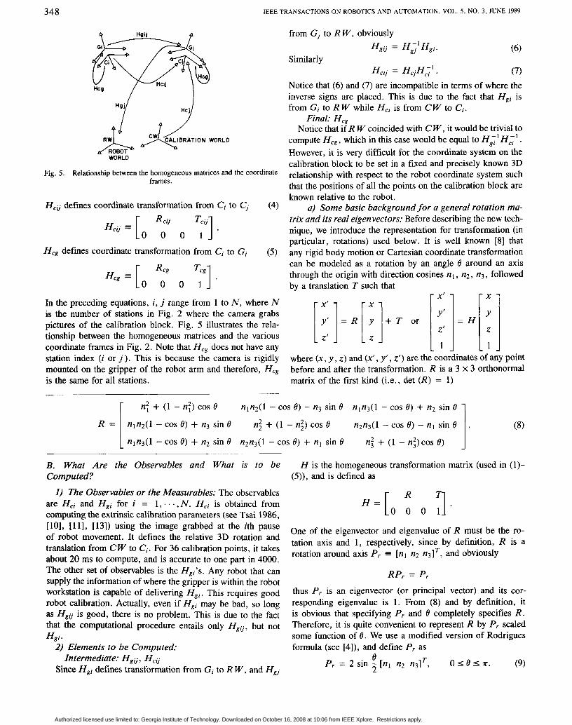
Fig. 5. Relationship between the homogeneous matrices and the coordinate frames.

Hcii defines coordinate transformation from C; to Cj (4)

Hcg defines coordinate transformation from C; to G; (5)

In the preceding equations, i , j range from 1 to N, where N is the number of stations in Fig. 2 where the camera grabs pictures of the calibration block. Fig. 5 illustrates the relationship between the homogeneous matrices and the various coordinate frames in Fig. 2. Note that Hcg does not have any station index ( i or j ) . This is because the camera is rigidly mounted on the gripper of the robot arm and therefore, Hcg is the same for all stations.

from Gj to R W , obviously

Similarly

Notice that (6) and (7) are incompatible in terms of where the inverse signs are placed. This is due to the fact that Hgi is from G; to R W while He; is from CW to C;.

(6) H .. = H I ’ H . g U SJ g r ‘

Hcjj = HCjHc;’. (7)

Final: He, Notice that if R W coincided with C W, it would be trivial to

compute Hcs , which in this case would be equal to Hgil He;‘ . However, it is very difficult for the coordinate system on the calibration block to be set in a fixed and precisely known 3D relationship with respect to the robot coordinate system such that the positions of all the points on the calibration block are known relative to the robot.

a) Some basic background for a general rotation matrix and its real eigenvectors: Before describing the new technique, we introduce the representation for transformation (in particular, rotations) used below. It is well known [8] that any rigid body motion or Cartesian coordinate transformation can be modeled as a rotation by an angle 0 around an axis through the origin with direction cosines n l , n2, n3 , followed by a translation T such that

r x ’ i r x i

where (x , y , z ) and (x’ , y ‘ , z’) are the coordinates of any point before and after the transformation. R is a 3 x 3 orthonormal matrix of the first kind (i.e., det (R) = 1 )

ni + ( 1 - nil cos e nln2( l - cos e) + n3 sin 0

nln3(1 - cos e) + n2 sin 8 n2n3(1 - cos e) + nl sin e

nln2(1 - cos e) - n3 sin e nln3(1 - cos e) + n2 sin e n2n3(l -cos e) - n l sin 8

ni + (1 - n:)cos e) n; + (1 - n;) cos 8

B. What Are the Observables and What is to be Computed?

I ) The Observables or the Measurables: The observables are He, and Hgr for i = 1, . . . , N. He, is obtained from computing the extrinsic calibration parameters (see Tsai 1986, [ lo ] , [ l l ] , [ 1 3 ] ) using the image grabbed at the ith pause of robot movement. It defines the relative 3D rotation and translation from C W to C, . For 36 calibration points, it takes about 20 ms to compute, and is accurate to one part in 4000. The other set of observables is the Hgl’s. Any robot that can supply the information of where the gripper is within the robot workstation is capable of delivering Hgl . This requires good robot calibration. Actually, even if Hgr may be bad, so long as HgIJ is good, there is no problem. This is due to the fact that the computational procedure entails only Hgr,, but not Hgr f

2) Elements to be Computed:

Since Hgr defines transformation from G , to R W, and Hg, Intermediate: HglJ, He,

H is the homogeneous transformation matrix (used in ( 1 ) - (5) ) , and is defined as

R

“ = [ o 0 0 3- One of the eigenvector and eigenvalue of R must be the rotation axis and 1, respectively, since by definition, R is a rotation around axis P , = [n l n2 n3IT, and obviously

RP, = P,

thus Pr is an eigenvector (or principal vector) and its cor- responding eigenvalue is 1. From (8) and by definition, it is obvious that specifying P , and e completely specifies R . Therefore, it is quite convenient to represent R by P , scaled some function of 8. We use a modified version of Rodrigues formula (see [4]), and define P , as

Pr = 2 sin - [nl n2 n31T, e o I e I T . (9) 2


TSAI AND LENZ: FULLY AUTONOMOUS AND EFFICIENT 3D ROBOTICS HANDIEYE CALIBRATION 349

Besides the advantages associated with quaternions or other vector representation of rotation matrix, one advantage for us is that some error formulas hold true even for noninfinitesimal perturbations. For example, Lemma V in Section III-A is exact. Also, the error formula in (29) is simpler. Another obvious advantage is that R is a simple function of P , without any trigonometric functions

1 2

R = (1 - q ) Z + - (P,P,T + CY * Skew(P,)) (IO)

where a = d m and Skew (Pr) is defined in (1 le). For the rest of the paper, the principal axis is defined as such, and all the computational procedures are given for P, explicitly, and not for R .

b) Computational procedures and conditions for uniqueness: We first give the computational procedures and conditions of uniqueness before we derive them. The derivations and proofs follow from the eleven properties or lemmas in Section 11-D. The actual proof for those eleven lemmas will be published in a later paper that will contain a fuller account of the work. The minimum number of stations is three, where station means the location where the robot pauses for doing camera extrinsic calibration. Using more than three stations improves the accuracy, as will be seen in Section 111-A.

Some Definition of Notation:

0 R : P,iJ :

Angle of rotation for R . Principal axis or rotation axis for R,, defined in (3), which is the 3D rotation from gripper coordinate frame Gi to G j , as defined in (3).

(1 la) P,, Rotation axis for R,, in (4). (1 1b) p e g : Rotation axis for R , . (1 IC)

- -q A /

(1 Id)

Skew (V): A skew-symmetric matrix generated by a 3D vector V such that

0 -Vz Vy

Skew (V) =

N. Number of stations described in Section 11-A.

Notice that the vectors defined above will also be used as a 3 x 1 column matrix. Also note that since Pg,, P,,, and P,, are rotation axes with a function of angle as their length, they completely specify Rgij, Re,, and R,. That is why for the procedures in the following, the formula for Peg is given, and not for R , .

3) Procedure for Computing Reg: Step 1: Compute P:g: For each pair of stations i , j such

Z L

X A y cw

Fig. 6. Pairs of stations should be selected such that the interstation angle is as large as possible, and the angle between different interstation rotation axes are as large as possible. The bar between stations denotes a particular selection of a pair of stations.

that the rotation angle R,, or R,, is as large as possible (Fig. 6 illustrates a good way to select the pairing. See also section on test results), set up a system of linear equations with pAg as the unknown

(12)

Since Skew (PglJ + PclJ) is always singular, it takes at least two pairs of stations to solve for a unique solution for p f g using linear least squares technique.

Exception handling: If P,, + P,, 1J is colinear with Pg,2, 2 + P,,2J2 while Pg, lJ 1 is not colinear with Pgr2/2, then the rotation angle of R , must be 180" and the rotation axis the same as Pgl

skew <'gIJ + pCIJ)p fg = pCIJ - p g l J .

+ P,, lJ . Step 2: Compute ORgc:

ORge = 2 tan-' lP:gl. (13)

Note: Step 2 is not quite necessary since P , in Step 3 is sufficient to represent rotation. However, (13) may be handy.

Step 3: Compute P,:

4) Procedure for Computing Tcg: Given at least two pairs of stations i , j, set up a linear systems of three linear equations with Tcg as unknowns

(15) For at least two pairs of stations, two sets of (15) are estab- lished and can be solved for the common unknowns Tcg using linear least squares solutions.

C. Speed Performance After the robot finishes the movement and grabbing the im-

ages, it takes only about 100 + 60N arithmetic operations to complete the computation. For a typical minicomputer, this only takes about 1/2 ms for ten stations. This complexity fig- ure (100 + 60N) can be derived as follows: The aajority

(Rgg - Z)Tcg = Rc,T,-Q - Tg,.



of the computation is for solving the overdetermined linear least squares solutions of (12) and (15). It takes about 3 X N x 32 to form the normal equation of either one of (1 le) and (16), and 33 x 2 to solve the 3 x 3 normal equation. With a minimum of three stations and two interstation pairs, it takes about 1/10 ms. This is negligible compared with the robot movement and image acquisition and analysis; at the pause of each movement, it takes about 90 ms to grab an image, extract all the 36 feature point coordinates with high accuracy, and compute the extrinsic camera parameters defined in (4).

D. Derivations of Computational Procedures and Conditions of Uniqueness using Eleven Lemmas

In order to outline the derivations of the computational procedures without going into actual details, eleven lemmas will first be stated and the significance of each explained. Selected sets of the key lemmas will be proved. Then the proof for the computational procedure for R , and Tcg will be given, followed by the conditions for uniqueness which will be stated and proved.

Lemma Z: Rgij and R c ~ differ by a unitary similarity transformation

(16) Proof: This follows easily from the fact that Hcg , Hg;; ,

H&', Hcjj in Fig. 5 form a closed loop and thus their product equals identity.

Significance: As a result, the eigenvector matrix of Rgii can be transformed from that of R,, using R,.

Lemma ZI: R , rotates the rotation axis of R,Q into that of

(17)

R .. = R R . . R T g U cg CIJ cg.

Rgij, or P g IJ ' . = RcgPc;j.

Proof: This follows from expanding R,ij and Rgij in (16) by their associated eigenvector and eigenvalue matrices, and making use of the fact that PgU and P,Q are the only real eigenvectors of Rg0 and R,,, respectively, and that the resultant rotation matrices on the left- and right-hand sides of (16) have a common real eigenvector.

Significance: Since, from Section 11-B1, Pcij and Pgij can be readily available from the observables H,ij and Hgij, (17) establishes constraints on Reg in order to solve for it. Lemma II also says that if we regard all P,o and Pgij as two clusters of vectors or points, then R , transforms one cluster into another.

Lemma IZZ: The rotation axis of R , is perpendicular to the vector joining the ends of the rotation axes for R,ij and

(18) Proof: This can be seen by observing Fig. 7, but alge-

braically, here is the proof (we will omit the subscript ij for clarity): The purpose is to show that (Pg - Pc)TPc = 0 . By making use of (17) and the fact that RcgPcg = Peg, we have

(Pg - P,)TPcg = (Pg - Pc) RcgRcgPcg

Rgij, or Pcg 1 (Pgij - Pcij).

T T

= (RcgRg - p g > T p c g

= [(Rcg - I)PgITP,

= P,'(R,T, -Z)Pcg = 0 .

Fig. 7 . Geometrical relationships between P,, P,, and P g . Peg rotates Pc into Pg . The plane containing the circle is perpendicular to P, , and point B is the midpoint of point C and G .

Significance: This implies that for a given pair of distinct PgU and PgO, Peg is confined to be in the bisecting plane of Pcij and PgU. With two such pairs, the direction of P , can be determined. In fact, (18) implies that Pcg can be determined up to a scale factor s from

However, we will not use Lemma I11 in this manner. Instead, Lemma I11 is used to build up the procedure for computing Reg via Lemmas IV, V, and VI. The reason is that (19) is more error-sensitive and has unnecessary degeneracies due to the fact that angle is not considered jointly.

Lemma IV: Pgii - Pcij is colinear with (Pgij + Pcij) x Peg. Proof: This follows from the fact that Pg;, - P,u is si-

multaneously orthogonal to Pcg (according to Lemma HI) and to Pgv + Pcii (this latter property can be easily proved).

Significance: This says that Pgc - P,u = s(Pgc + P,Q) x Peg for some scale factor s. Lemma V forces s to be 1. This lemma makes use of Lemma LII, but the formula it generates is more accurate and robust than (1 8) (coming out of Lemma III) so far as computing P , is concerned, as will be seen.

Lemma V: Pgij - P,, and (PgU + PcU) x P i g have the same length, where P i g was defined in (l ld).

Proof: Again, in the following proof and in Fig. 7, we will drop the subscript i j for P g ~ and Pcij. Let the angle between the vectors represented by P i g and Pg + P, be a. Then by definition

J(Pg + P,) x P i g \ = 1pg + P , J / P ; ~ J sin a.

Pcg = NPgi, j , - Pci, j , ) x (Pgi, j , - Pciz j 2 ) . (19)

Substituting (9) and (1 Id) into the above gives 6 2

l(Pg + P,) x P & = lpg + ~ , 1 2 sin - -1/2

* (4 - 4 sin2 ;) sin a

6 2

= IPg + P,I tan - sin a

= 210B1 sin atan -

= 2 1 2 B tan - = 21cBI

= JCGJ = JP, - PCJ.

6 2

6 2


TSAI AND LENZ: FULLY AUTONOMOUS AND EFFICIENT 3D ROBOTICS HANDEYE CALIBRATION 35 1

In the above derivations, A , B, C , G , 0 are points in Fig. 7, and /OB/ means length of the vector extending from point 0 to point B, etc. Also, in the above derivations, several geometric and trigonometric relationships in Fig. 7 are used. One is lPg + P,I = 210BI. Another is sin a.

Still another is 1-1 = tan 0/2. These properties follow easily from Fig. 7. Thus we have shown that

=

I(P, + Pc) x pig1 = lPg -Pel. Significance: Given Lemmas IV and V, Lemma VI is

readily derived, which easily leads to the computational procedure for p,, in (12).

Lemma VI:

(PgQ + PcQ) x P & = P,, - PgQ.

Proof: This is a direct consequence of Lemmas IV and V.

Significance: Although (18) provides a constraint on the direction of P , for any pair of stations ij, (20) provides a stronger constraint since it constrains 6Rcg as well as Pcg.

Lemma VZZ: Skew ( P g ~ + P,u) is singular and has rank 2.

Significance: Skew (Pgu + P,u) is the coefficient matrix for the systems of linear equations in (12) used to solve for PA,. Therefore, Lemma VI1 implies that it is impossible to compute R , with only two stations.

Lemma VZZZ:

(Rgij - Z)Tcg = Rcg Tcjj - Tg;j. (21) Proof: This follows from the same derivation as

Significance: Lemma VIII establishes the equation in Lemma I.

(1 5 ) used to solve for T,, . Lemma ZX: R,Q - Z is singular and has rank 2.

Significance: R,Q - Z is the coefficient matrix for the systems of linear equations in (15) used to solve for Tcg. Therefore, Lemma IX implies that it is impossible to compute Tcg with only two stations.

Lemma X: If OR, # s, or equivalently, IP,,l # +- 2, then

has full column rank if and only if Pgi, j l and Pgi2j2 have different directions (or equivalently, PCi, j l and PCj2j2 have different directions).

Significance: Expression (22) is just the compound matrix of two Skew ( P g ~ + p , ~ ) in Lemma VII, and therefore is the coefficient matrix for solving R , given two pairs of PgQ and PCi,. Thus Lemma X ensures that given a minimum of three stations, the solution for R , is unique.

Lemma XI:

has full column rank if and only if Pg; , j l and Pgj2j2 have different directions (or equivalently, P,;, j , and PCi2jz have different directions).

Significance: Expression (23) is just the compound matrix of two R,;j - Z in Lemma IX, and therefore is the coefficient matrix for solving Tcg given two pairs of Psi and PCjj . Thus Lemma XI ensures that given a minimum of three stations, the solution for Tcg is unique.

Proof of the Computational Procedure for R,, in (12)- (14): Equation (12) follows from Lemma VI by considering the fact that for any two 3 x 1 vectors a and b

a x b = Skew(a) b (24)

where a and b on the left denotes vectors while a and b on the right are 3 x 1 column matrices. Equations (13) and (14) simply follow from the definitions of P i , in (l ld).

Proof of the Computational Procedure for Tcg in (15): This follows simply from Lemma VIII.

Minimum Number of Stations: Three. This follows from Lemmas VII, IX, X, and XI. Equivalently, the minimum number of pairs of stations needed is two.

Conditions of Uniqueness: For a minimum of three stations (or two pairs of stations), the necessary and sufficient condition for a unique solution for R,, and T,, is that the interstation rotation axes are not colinear for different pairs of stations.

Proof: This follows from Lemmas X and XI. Note that when the sum of rotation axes (Pgu + PCu) are colinear while P g ~ is different for different interstation rotations, then the solution is still unique except that (12) cannot be used. In this case, angle (R,,) is simply 180" and the rotation axis is the same as Pcu + P,Q.

111. ACCURACY ISSUES

In the following, error analysis will first be given. Then, as a result of error analysis, critical factors dominating the error, and steps for improving accuracy will be described.

A. Error Analysis The purposes of error analysis are as follows: 1) It reveals what the critical factors influencing the accu-

2) It gives rise to various means for improving accuracy. 3) It is essential for accuracy prediction, which is important

to model-driven 3D vision planning. 4) It helps to determine whether one has properly imple-

mented the algorithm. If the error is much larger than what the error formula predicts, something in the setup, programs, or system are not in the right order.

In this section, we first give a list of definitions, followed by a list of lemmas used for deriving the final error formula for R,, and Tcg. Then the error formula for R,, , T,,, and R,,, Tgjj due to error of R,;, TCi and Rgi, T,; will be given, followed by the error formula of R , and Tcg . Critical factors affecting the accuracy will be discussed in the next section, and test results will follow thereafter. Definitions:

RMS:

u(V) :

racy are.

Root mean square (or average of the sum of squares). RMS of the magnitude of error corrupting a 3D vector V . a( V ) and uv are equivalent.


IEEE TRANSACTIONS ON ROBOTICS AND AUTOMATION, VOL. 5 , NO. 3, JUNE 1989 352

a(R):

Err ( V ) :

Err (R):

RMS of the magnitude of error of PR (rotation axis scaled by the rotation angle, see (6), (1la)- (Ilc)). a(R) and UR are equivalent. Maximum magnitude of error corrupting a 3D vector V. Maximum magnitude of error for PR.

List of Lemmas Leading to the Final Error Formula Lemma I:

PAR.R = P A R + PR where A R is a small perturbation rotation matrix.

rotation, the rotation axes are additive. Note: Lemma I says that for small error perturbation of

Lemma 11:

4 R 1 R 2 ) = w. Lemma 111:

Err ( R I R 2 ) = Err ( R I ) + Err (R2) .

Lemma IV:

where V ] are a number of 3D vectors with RMSE av,. Lemma V:

a(R ' v ) =./: (0~1 VI)' + U,?

where R is a rotation matrix with RMSE OR and V is a 3D vector with RMSE av.

Lemma VI:

Err (E Vi ) = E Err (Vi). I

Lemma VII:

Err (RI / ) = Err (R)IV/ + Err ( V ) .

The proof for the above Lemmas will be published in a later paper. The following formulas can be easily derived from the above lemmas and the relationships between R, , and Rei, R , and between T,, and Rei, Tc; using (12).

Error of Rev due to Error of Rei and R,j

' R , , = dui,, (254

Err (Rely) = Err (Rei) + Err (Rcj). ( 2 3 9 Similar formulas hold for R, .

Error of TCb due to Error of Rci and Tci

Equation (26b) is a simpler version of (26a) with u R ~ , and uR, replaced by u R ~ , etc.

Err (T,ij) = [Err (Rei) + Err (Rcj)]lTcil

+Err (Tci) + Err (Tcj). (26c)

Error of Tgii due to Error of R,i and Tgi

=./i ui,lTgl - Tg212 + 20;~ (27b)

Err (Tgu) = Err (Rg2)JTgl - Tg21 +Err (Tg1) +Err (Tg2).

(27c)

Error of R , Three-Station Case:

where / ( P g I 2 , Pg23) means the angle between Pg12 and Pg23

eRgI2/2 = 21Pg121 = angle (Rg12)/2.

Note that

arrangement in Section IV), (28a) reduces to

= OR,,] for all i j . Since it is always easy to have f?Rglz close to ORgz3 (see the

ri


TSAI AND LENZ: FULLY AUTONOMOUS AND EFFICIENT 3D ROBOTICS HANDEYE CALIBRATION 353

where Xi’s are the singular values of a matrix with the rows being the interstation rotation eigenvectors (using definition in (9)) for the camera. A few facts are worth noting (details and proofs to be published). First is that as the interstation rotation angle increases, Xi increases linearly, making uRCg inversely proportional to the interstation rotation angle. The second and most important fact is that as the number of interstation rotations N increases hi increases by the square root of N, making uR, inversely proportional to a. Similarly

Err (Reg) = (Err ( R g d + Err (Red

Error of Tcg Three-Station Case:

where

and is the coefficient matrix for solving Tcg in (15); and cond (A) is the condition number of A and is defined as

cond (A) = 11 A 11 - /I A-’ 11 . To simplify the formula, we can regard as being close in magnitude, and IT,i - Tgil as being close in magnitude, making (31) somewhat simpler:

Similarly

The effect of the number of stations on the error is the same as that for R,,. This is verified by the test results in Section IV . B. Critical Factors Affecting the Accuracy and Steps in Improving Accuracy

By observing the accuracy formulas for R, and Tcg in Section III-A, the following observations can be made:

Observation 1: The RMS error of rotation from gripper to camera uR, is inversely proportional to the sine of the angle between the interstation rotation axes.

By observing (28a), it is seen that uRCg is inversely proportional to sin (L(Pg12, Pg23)) (which is equal to sin (L(Pc12, Pc23))). This is reasonable since, from Lemma I1 in Section LI-D, R, rotates P,,, into PE,,. With a minimum of two pairs of ij ’s, (17) is used to solve for R,. When /(Pg12, Pg23) becomes smaller, Pg12 becomes closer to Pg23, making (17) for each ij more similar to each other, thus causing the equation to be closer to singularity. Alternatively, one can see that the coefficient matrix for solving P & (see L.emma VII in Section II-D) becomes singular as P,,, approaches Pg,, J Z and P,,, ,, approaches P,,, /,. In fact, it can be shown that the row vectors of the coefficient matrix in Lemma X lie in two planes, with Pg,, + P,,, and Pgr2 J z + P,,, J 2 being the normal vectors of the two planes. Thus the greater the difference between P,,, J ,

and P,,, J z , the closer the two planes are to being orthogonal, making the coefficient matrix more linearly independent.

Observation 2: The rotation and translation error are both inversely proportional to the interstation rotation angle. That is

uR, OC -1 eRg,J and UTcg OC - 1 e R , , . This can be seen from (28c), (28d), and (31). This is reasonable since R, is determined solely from PclJ and PgU, and the greater and 8Rgr1 are, the smaller the effect of a small perturbation (with given size U R ~ , , , uRglZ) is on the result.

Observation 3: The distance between the camera lens center and the calibration block has a dominant effect on the translation error. This comes from (31)-(33). In fact, any of the terms in (31) or (32) involving 1 T,,I or 1 Tgl - Tg21 generates much more error than all other terms in most of the practical setup. For example, if ITC1I is 5 in and the error of interstation rotations is 3 mrad (these are practical figures that one would encounter), then any term in (31) or (32) involving u ~ ~ I T ~ ~ ~ would generate 15-mil error, which is much bigger than those other terms involving UT,, which is the error of translation as a result of extrinsic camera calibration. The term involving UT^, however, has the potential of being very big, since this depends on the positional accuracy of the robot, which can be bad.


354 IEEE TRANSACTIONS ON ROBOTICS AND AUTOMATION, VOL. 5 , NO. 3 , JUNE 1989

Observation 4: The distance between the robot gripper coordinate centers at different stations is also a critical factor in forming the error of translation. But the distances between different camera stations are not important.

This again comes from (31)-(33). The situation is similar to that described in Observation 3. Notice that lTgl - Tg21 is not the distance between gripper tips at different stations. It is the amount of movement of the robot gripper coordinate center.

Observation 5: The error of rotation is linearly proportional to the error of orientation of each station relative to the base. The error of translation is approximately linearly proportional to this error of orientation unless the error of robot translational positioning accuracy is big.

This comes from (28c), (28d), and (31)-(33). It is convenient to define two types of critical factors. One

is first-degree, and the other second-degree. The first-degree factor is more dominant in most cases, but sometimes, some second-degree factor UT^^) can be so bad that it becomes dominant.

First-Degree Critical Factors:

1) The angle between different interstation rotation axes (e.g., ~ ( P ~ 1 2 , p g 2 3 ) ) . Note: W g 1 2 , p g 2 3 ) = L(Pc12,

2 ) The rotation angle of interstation rotation = 6 R c , l ) . 3) The distance between the camera lens center and the cal-

ibration block 1 Tcil, and the distance between the robot- arm coordinate centers at different stations I Tgl - Tg2 1 .

4) The error of rotation of each station relative to base UR,, , uR,, , or error of interstation rotation UR, ,~ , UR~, , .

pc23 ).

Second-Degree Critical Factor:

1) Error of translation of each station relative to base UT^, , UTg,.

C. Steps to Improve Accuracy 1) Adopt the setup to be described in Section IV in or-

der to achieve maximum angles between different interstation rotation axes, no matter how many stations are used.

2) Maximize the rotation angle for interstation rotations. This again can be done using the setup mentioned earlier.

3) Minimize the distance between the camera lens center and the calibration block. This requires a small calibration block and suitable optics for short-range viewing.

4) Minimize the distance between the robot arm coordinate centers at different stations. This requires some planning and is robot-dependent.

5 ) Use redundant stations. The setup described in Section IV is ideal for using as many stations as you wish. Since the extrinsic calibration plus feature extraction can be done within 90 ms when 36 points are used, using more frames poses no problem. The error due to nonsystematic sources will be reduced by a factor of a where N is the number of stations. (See results in Section IV.)

6) Use camera calibration algorithm setup that yields high

accuracy to improve error on translation and rotation of each individual station.

7) Try to precalibrate the robot itself so that the position and orientation of each station is known more accurately. If this is difficult, then at least try to make interstation translation and rotation more accurate, if possible. That is, the robot system may not be able to tell the user the absolute location and orientation of its gripper coordinate frame, it may, however, be able to better tell the amount of relative movement from station to station.

IV. SIMULATION A N D REAL EXPERIMENT RESULTS A. Simulation Experiments

I ) The Station Generation Process: It is important to use a process for simulating the position and orientation of gripper and camera stations that is realistic and easy for controlling the critical parameters of Section lU-B in order to see their effect on the final accuracy. It should allow all critical parameters to be in optimum conditions simultaneously. It also serves as a means of planning robot motion in order to generate stations in the real experiments. Fig. 6 illustrates the results of using our process for generating a five-station configuration. The bright coordinate frames are the camera coordinate frames Ci while the darker frames are for the robot gripper coordinate frames Gi. The bars in Fig. 6 indicate the selections of interstation pairs. The station generation process is described as follows: first, set up a calibration block world coordinate frame C W and a robot world coordinate frame R W as in Fig. 6. Next, directly above C W , place a pair of coordinate frames CO and Go for camera and gripper that maintains a distance of I Tcl from C W (notice that I Tc I is one among the critical factors in Section 111-B) with the z axis of CO pointing right at C W . CO and Go are actually not used for computing the results R, and T,,, but rather for generating other stations. Next, select a number N to be the total number of stations to be generated. Then, generate N stations for camera and gripper by rotating CO and Go around N axes uniformly distributed with 360/N degrees apart, centered at C W and parallel to the xy plane of C W . The interstation pairs are chosen using a star-drawing technique (see Fig. 6). This gives a systematic way of generating an arbitrary number of stations while at the same time allowing one to easily vary the critical parameters for testing error sensitivity.

2) The Control of Critical Parameters as Simulation In- put Parameters: All of the critical parameters (first and second degree) listed in Section 111-B can be simulated with easy control. The control of each critical parameter is listed in the following:

Interstation rotation angle: This is controlled by varying the rotation angle used in rotating CO and Go to each individual station.

Angle between different interstation rotation axes: This is controlled actually by varying the number of stations generated. For each case, choose only the first three traversed by doing star drawing. Obviously, the larger the number of overall stations is, the narrower the angle between successive interstation rotation axes is.

Distance between camera and calibration block: This


TSAI AND LENZ: FULLY AUTONOMOUS AND EFFICIENT 3D ROBOTICS HAND

14 -

3 ::: H e e -

4 -

2 -

0 2 ‘ 4 6 8 10 0

INVERSE OF INTER-STATION ROTATION ANGLE (1/RM)

Fig. 8. angle.

is controlled by varying the distance IT, I in the above generation procedure for placing CO and Go.

Number of stations: This is the parameter in the process that is totally arbitrary, except that if it is even, the star drawing is not as straightforward. We always use an odd number of stations.

Rotation and translation error for each station ( u R ~ , , UT^,, U R ~ , , and UT^,): This is an extrinsic calibration error, and can be simulated by perturbing the ideal homogeneous transformation matrices for each station. From our simulation tests, they agree quite well with Section HI-B.

Fixed setup parameters: In order to simulate the actual physical setup, all the setup parameters are selected to be almost the same as those used in the real experiments to be described, except that due to the x axis problem with our robot (to be described later), the station generation process used in the real experiment is modified. In the following, the setup parameters are set as follows:

RMS rotation error as a function of inverse of interstation rotation

ITcl = 6.65in ITcg[ = 9.5in

N = 3 UTc, = 3

UTg, = 5 mil U R ~ , = U R ~ , = 1.511~ad.

In the following, we show the simulation results of four critical parameters on the error of rotation R , and translation Tcg. These four critical parameters are tested separately. For the testing of each parameter, all the other setup and critical parameters are set as above, while the very parameter under test will be allowed to vary over a given range. loo0 tests are done for each case, and statistics are gathered. The results are shown in the following figures.

3) Simulation Results: Effect of the size of interstation rotation angle on ac-

curacy: Section 111-B described the relationships between the size of the interstation rotation angle and the R , as well as Tcg accuracy, and gave procedures for improving the accuracy. Extensive simulation has been done and the results are consolidated into Figs. 8 and 9 (one for rotation error and the

‘EYE CALIBRATION 355

0 2 4 6 8 10

INVERSE OF ANGULAR STATION SPREAD (l/RAD)

RMS translation error as a function of inverse of interstation rotation Fig. 9. angle.

0 5 10 15 20 25 IENERSE OF ANGLE BETWEEN W O R ROTATON AXIS (pi/RAD)

Fig. 10. RMS rotation error as a function of inverse of angle between two different interstation rotation axes.

other translation). The curve is linear up to statistical sampling tolerance. It agrees quite well with Observation 2 in Section III-B, and it confirms the recommendation made in Section III- C.

Effect of angle between interstation rotation axes on accuracy: The situation is similar to that above except that L(Pg12, PpgZ3) is allowed to vary while ORgl2 and ORgz3 are fixed. Fig. 10 shows the average error of rotation as a function of L(Pg12, Ppgz3). It is again linear, as predicted in Lemma I.

Effect of camera-to-calibration-plate distance on accuracy: According to (31), the translation error has a dominant effect on unless UT,, or UT^, are enormous. Fig. 11 reflects this quite well. The RMS error of Tcg is plot- ted against this parameter. The curve is generally linear, but around the origin, it bends somewhat, due to the fact that when I TcI is small, its effect is no longer dominant and the effect of UT^, shows up.

Effect of number of interstation pairs on accuracy: Figs.


356 IEEE TRANSACTIONS ON ROBOTICS AND AUTOMATION, VOL. 5, NO. 3, JUNE 1989

" 0 2 4 6 6 1 0 1 2 1 4

D~STANCE FROM CAMERA TO CAUBRAIION BLOCK (INCHES)

Fig. 11. RMS translation error as a function of the inverse of distance between camera and calibration plate.

" 0.0 0.1 0.2 0.3 0.4 0.5 0.6

INMRSE OF %WE ROOT OF NUMBER OF SlAllloNs

Fig. 12. Translation error as a function of inverse of square root of the number of interstation pairs. The solid line is RMSE and dashed line is maximum error.

12 and 13 show the error of translation and rotation as a function of the inverse of square root of the number of interstation pairs. The solid line shows the RMS error, while the dashed line is the maximum error out of one thousand tests. As ex- pected, the RMS error increases linearly as the inverse of &. Since the proposed technique is quite efficient, and the station pose planning and robot motion are automatic, increasing the number of stations is quite feasible, and pays off well.

B. Real Experiments I ) Setup Description: Fig. 3 shows the physical setup we

used. A Javelin CCDE 480 x 388 camera is fastened to the last joint of an IBM Clean Room Robot (CRR). The CRR has two manipulators, each with seven degrees of freedom (including gripper opening). We only use one of the manipulators. The CRR is an electric box frame Cartesian robot. There are three linear joints (x , y, z) and three rotary joints (roll, pitch, and yaw) for each manipulator. The work volume is about 6 ft

0.0 0.1 0.2 0.3 0.4 0.5 0.6 INMRSE OF SQUARE ROOT Of NUMBER OF STATIONS

Fig. 13. Rotation error as a function of inverse of square root of the number of interstation paris. The solid line is RMSE and dashed line is maximum error.

by 4 ft by 2 ft and the repeatability for linear joint is about 4 mil, and that for the rotary joints 1 mrad. The accuracy is calibrated to a limited extent. The scale and offset for each rotary joint are calibrated to 3-mrad accuracy. The rotation axes for the three rotary joints are supposed to be intersect- ing at the same point (origin of R W coordinate frame), but we did not calibrate that. The x axis has some problems: For our robot, the z beam sags, causing the movement in the x axis to be like that of a pendulum. This effect is not fully calibrated yet, but we suspect that it generates about 20-mil translation and 15-mrad rotation within a work range of 15 in. Due to this problem, we are forced to modify the station generation procedure used in the simulation in order to avoid using the x axis. Either with or without moving the x axis, the station placement and manipulator motion planning is automatic, and the number of stations can be arbitrary without manual intervention.

The calibration block is a clear glass plate with the center 1 in by 1 in area filled with 36 black discs printed on it using step-and-repeat photographic emulsion (see Fig. 14). The discs are 5000 pm apart with 2000-pm radius (accurate to 1 pm). The calibration is back-lighted and sits in the middle of the work space.

2) Accuracy Assessment: The accuracy of our handleye calibration results is assessed by how accurately we can predict the placement of a camera in 3D world with any arbitrary manipulator movement. As was indicated in Section I-D, one of the main reasons why robot handleye calibration is important is that the robot needs to know not only where the gripper is, but also where the camera is in the work space, so that the measurement taken by vision can be related to the robot. Be- ing able to determine where the camera is in the work space for an arbitrary manipulator movement is thus the primary goal. This is tested in the following steps:

Step 1: Move the manipulator to 2N different positions where N is greater than 2. For each station i , compute the camera to calibration block homogeneous transformation f f c i

using extrinsic calibration. This takes about 90 ms per station.


TSAI AND LENZ: FULLY AUTONOMOUS AND EFFICIENT 3D ROBOTICS HANDIEYE CALIBRATION 357

Fig. 1 Calibration block is a clear glass plate with 36 discs printe using photographic emulsion. The accuracy is 4 pm.

m it

The robot gripper position and orientation relative to robot world, which is Hgi, is also recorded.

Step 2: Compute Hcg using procedures in Section II- B2b, using data from stations 1 through N .

Step 3: For each station k (k from 1 to N ) compute the homogeneous matrix HRC (homogeneous transformation from robot world frame R W to calibration block world frame C W ) by

~ : l ~ - l ~ - l HRC = C, cg g; .

Make an average of HRC computed from these N stations. Step 4: Let stations N + 1 through 2N be called verifi-

cation stations. For each of the verification stations, predict the position and orientation of the camera relative to the robot world base coordinate R W by HG‘ Hgi’ where k is the station index, and Hgk is computed from robot joint coordinates (see Section 11-B). Compare this predicted position and orientation with HckHRC, where Hck is computed in step 1 while HRC is computed in step 3.

The results of a series of experiments yield the following table:

New Camera Pose Prediction Error N Rotation Error (mrad) Translation Error (mil)

4 6 8 10 12

4.568 3.304 3.264 2.888 2.782

23.238 19.078 26.712 14.642 12.516

Since there is no absolute Hcg ground truth to compare with, the accuracy has to be assessed as the error of new camera pose prediction, as described earlier. The effect of N is indeed very significant. We have a program that automatically plans the movement of the manipulator for an arbitrary number of stations, and since the algorithm proposed in this paper is quite efficient, increasing the number of frames is quite easy. Also observe that the error of the predicted camera pose includes both the error of the calibrated hand/eye relationship and the robot’s positioning error. Notice from the table that for 10 stations, the translation error is about 14 mil. But the robot’s positioning accuracy is worse than 10 mil. This means that the eye-to-hand relationship is calibrated to better than 10 mil. Using the error formula in (32) scaled by J10/3, the error fo Tcg is predicted to be 10.66

mil, agreeing well with the real experiment data. The rotation error is about 2.88 mad. Notice that the error of rotary joint is about 2.5 mrad. Therefore, the actual error of Rcg should also be of this order of magnitude. This agrees very well with the prediction by (28), which gives 2.557 mrad. Notice that the error in the table is not strictly monotonic with respect to the inverse of the square root of number of stations. This is due to the fact that the simulation curves presented earlier were averaged over lo00 tests, while here, for each N , there is only one test. Also, since the robot error itself gets into it, it is more unpredictable, while the simulation curves only show the Hcg error. Nevertheless, the error generally decreases nicely as the number of stations increases.

V. CONCLUSION

This paper introduced a high-speed, high-accuracy, versatile, simple, and fully autonomous technique for 3D robotics hand/eye calibration. It is high speed since it takes only about 100 + 64N arithmetic operations to compute the hand/eye relationship after the robot finishes the movement, and incurs only additional 64 arithmetic operations for each additional station. This makes the current algorithm the fastest compared with the state of the art. The speed performance is especially attractive to those applications where the hand/eye configuration needs to be changed frequently. For example, the robot may pick up the camera to perform some task, and then put it right back to a holder. Since the grasping cannot be precise, hand/eye calibration must be performed frequently. It is also important to those tasks where hand/eye relationships need be changed frequently due to different task requirements. As for the accuracy, no other reported hand/eye calibration technique does any better. The results in our real experiments could be further improved if we changed the optics and the size of calibration block, as well as the mounting position, so that all of the critical factors described in the accuracy analysis section would be taken into consideration.

REFERENCES

M. Bowman and A. Forrest, “Robot model optimization,” submitted for publication, 1987. K. S. Fu, R. C. Gonzalez, and C. S. G . Lee, Robotics: Control, Sensing, Vision and Intelligence. New York, NY: McGraw-Hill, 1987. A. Izaguirre, J . Summers, P. Pu, “A new development in camera calibration, calibrating a pair of mobile TV cameras,” to appear in Int. Robotics Res., 1987. J. L. Jenkins and J. D. Turner, OptimalSpacecraft RotationalMan- ervers. R. Lenz and R. Y. Tsai, “Calibrating a Cartesian robot with eye- on-hand configuration independent of eye-to-hand relationship,” in Proc. IEEE Computer Vision and Pattern Recognition Cont. (Ann Arbor, MI, June 5-9, 1988). - , “Techniques for calibration of the scale factor and image center for high accuracy 3D machine vision metrology,” in Proc. IEEE Int. Conf. on Robotic and Automution (Raleigh, NC). Also to appear in IEEE Trans. Pattern Anal. Mach. Intel. G . Puskorius and I. kldkamp, “Calibration of robot vision,” in Proc. IEEE Int. Conf. on Robotic and Automation (Raleigh, NC, 1987). D. F. Rogers and J. A. Adams, Mathematical Elements for Com- puter Graphics. Y. Shiu and S. Ahmad, in Proc. IEEE Int. Conf. on Robotic and Automation (Raleigh, NC, 1987). R. Tsai, “A versatile camera calibration technique for high accuracy 3D machine vision metrology using off-the-shelf TV cameras

Amsterdam, The Netherlands: Elsevier, 1986.

New York, NY: McGraw-Hill, 1976.



and lenses,” IEEE J. Robotics Automat., vol. RA-3, no. 4, Aug. 1987. A preliminary version presented at the 1986 IEEE International Conference on Computer Vision and Pattern Recognition, Miami, FL, June 22-26. R. Tsai and R. Len, “Review of the two-stage camera calibration technique plus some new implementation tips and new techniques for center and scale calibration,” presented at the Second Topical Meeting on Machine Vision, Optical Society of America, Lake Tahoe, Mar.

-, “A new technique for fully autonomous and efficient 3D robotics hand-eye calibration,” in 4th Int. Symp. on Robotics Re- search (Santa Cruz, CA, Aug. 9-14, 1987). -, “Review of RAC-based camera calibration vision,” Society of Manufacturing Engineers, Nov. 1988. - , “Real time versatile robotics hand/eye calibration using 3D machine vision,’’ presented at the Int. Conf. on Robotics and Automa- tion, Philadelphia, PA. Apr. 24-29, 1988. - , “Three-dimensional mechanical part measurement using a vision/robot system,” IBM Res. Rep. RC 10506, May 8, 1984.

18-20, 1987.

Roger Y. Tsai received the M.S. degree from Pur- due University, W. Lafayette, IN, and the Ph.D. degree from the University of Illinois at Urbana- Champaign, both in electrical engineering, in 1980 and 1981, respectively.

He was employed by Bell-Northern Research/ INTS-Telecommunications, Montreal, Canada, for three months during the summer of 1979 as a Vis- iting Scientist, working on moving image registra- tion and enhancement. During the summer of 1980, he was employed by the Signal Processing Group,

EPFL, Lausanne, Switzerland, for three months working on 3D time-varying scene analyses. In the summer of 1981, he again visited BNWNRS, Mon-

treal, for three months, working on image sequence analysis and computer vision. He is now with IBM T. J. Watson Research Center, Yorktown Heights, NY, where he has been initiating and leading projects in the area of 3D machine vision. He was the recipient of the Best Paper Award for 1986 IEEE International Conference on Computer Vision and Pattern Recognition (CVPR) and the 1986, 1987, and 1988 IBM External Honor Recognition. He is the Technical Editor of Robotics Vision and Inspection System for IEEE TRANSACTIONS ON ROBOTICS AND AUTOMATION. He has served as chairman of the Computer Vision committee for the IEEE Society of Robotics and Automation for 1988. He served on the program committee for 1989 IEEE Int. Conf. CVPR, and has served as session chairman for 1986 IEEE Intern. Conf. on CVPR, 1987 and 1988 IEEE International Conference on Robotics and Automation. He is on the editorial board for Robotics Review (MIT Press). His major research interests include 3D robotics and geometric vision, sensor planning, modeling and calibration, 3D stereo measurement, inspection, automated assembly, etc.

Reimar K. Leoz was born in Aachen, W. Germany, on January 10, 1956. He received the B.S. degree from the TU Stuttgart in 1977, the M.S. and Ph.D. degree from TU Munchen, in 1980 and 1986, respectively, all in electrical engineering. His Ph.D. dissertation was on fast algorithms to estimate gw- metric transformations in image sequences.

Since 1980 he has been a Research Assistant at the Lehrstuhl fiir Nachrichtentechnik in Munich, in- terrupted by research assignments at the Lehrstuhl fiir Theoretische Nachrichtentechnik in Hannover in

1981. (Data Compression, 64 With TV) and at the IBM T. J. Watson Re- search Center, Yorktown Heights, NY, during 1986 and 1987 (Manufacturing Research, Robot Vision, Real-Time Vision). His current research interests are camera calibration and pattern recognition.


Documents

1989 A New Technique for Fully Efficient 3Dkmlee.gatech.edu/me6406/handeye.pdf · A New Technique for Fully Autonomous and Efficient 3D Robotics Hand/Eye Calibration ... and equal