1999 CAS SEMINAR ON RATEMAKING

OPRYLAND HOTEL CONVENTION CENTER

MARCH 11-12, 1999

MIS-43

APPLICATIONS OF THE MIXED EXPONENTIAL DISTRIBUTION

CLIVE L. KEATINGE AND JOHN NOBLEInsurance Services Office

Features of the Mixed Exponential Increased Limits Procedure:

• Ability to include Excess, Umbrella, and Deductible data.

• Ability to treat policy limit censorship without an a priori distribution assumption. Promotes clarity in evaluating various distribution fits.

• Ability to reflect differences in severity distributions by policy limit.

• Use of mixed exponential distributions instead of mixed Pareto distributions. Allows closer fits to the underlying data.

• Lack of constraints across increased limits tables.

The two main steps of the mixed exponential increased limits procedure are:

1. Constructing an empirical distribution

2. Fitting a mixed exponential distribution to

an empirical distribution

Constructing an empirical distribution

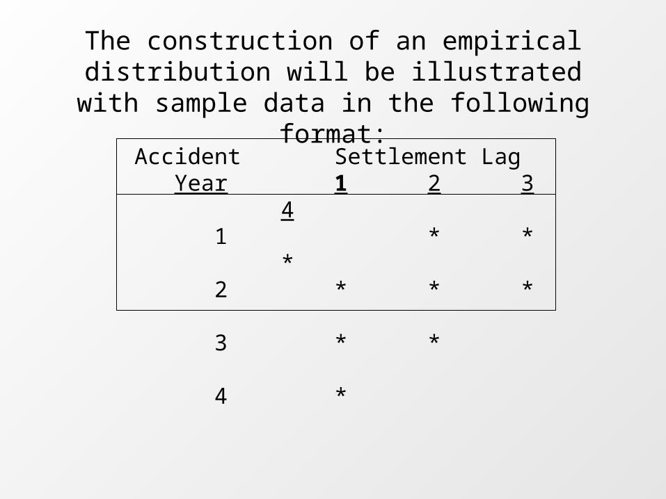
The construction of an empirical distribution will be illustrated with sample data in the following format:

Accident Settlement Lag Year 1 2 3 4 1 * * * 2 * * * 3 * * 4 *

Each * represents the collection of all settled occurrences in that cell.

Each cell contains all occurrences settling at that lag for that accident year. A calendar accident year occurrence settling between January 1 and December 31 of that same year is defined to have settled in Lag 1.

Settlement Lag = Average Payment Year - Accident Year + 1

As a first step, all settled occurrences are trended to the average accident date for which a loss distribution is desired allowing us to combine data for all accident years within each lag. Later, distributions for each lag will be weighted together to implicitly account for development.

Data from each lag must be treated separately because:

1. Later lags tend to have a greater percentage of large losses than earlier lags since occurrences that take longer to settle are generally more severe than claims that settle quickly.

2. The particular lag’s data includes different groups of accident years which likely have different exposure amounts. This will be addressed in the lag weighting procedure.

For each lag, we want to obtain the empirical survival function (survival probability) at a number of different dollar amounts.

Survival Function = S(x) = 1 - Cum. Distribution Function = 1 - F(x)

The survival probabilities at each dollar amount will be derived (‘built-up’) using a series of conditional survival probabilities (CSP’s).

This will allow us to more easily include:

1. Losses Censored by Policy Limit

2. Excess, Umbrella and Deductible data

3. Composite-Rated Risks data

To obtain the empirical survival function, we will use a variation of the Kaplan-Meier Product-Limit Estimator. This has historically been used extensively in survival analysis. For further details see:

Loss Models: From Data to Decisions, by Klugman, Panjer and Willmot

Survival Analysis: Techniques for Censored and Truncated Data, by Klein and Moeschberger

Both of these texts will be used for CAS/SOA Exams 3 and 4 beginning next year.

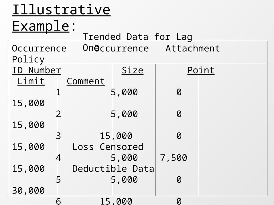
Illustrative Example:Trended Data for Lag One

Occurrence Occurrence Attachment PolicyID Number Size Point Limit Comment 1 5,000 0 15,000 2 5,000 0 15,000 3 15,000 0 15,000 Loss Censored 4 5,000 7,500 15,000 Deductible Data 5 5,000 0 30,000 6 15,000 0 30,000 7 25,000 0 30,000 8 10,000 15,000 30,000 Excess Data 9 15,000 0 100,000 10 25,000 0 100,000 11 30,000 0 100,000 12 50,000 15,000 100,000 Excess Data

• We will obtain the empirical survival function at the following dollar amounts:

10,000 20,000 40,000

• These survival probabilities will be derived by multiplying the relevant conditional survival probabilities (CSP’s) for each dollar amount.

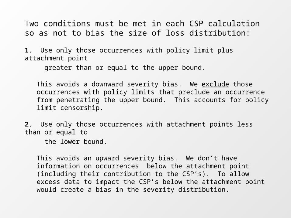
Two conditions must be met in each CSP calculation so as not to bias the size of loss distribution:

1. Use only those occurrences with policy limit plus attachment point

greater than or equal to the upper bound.

This avoids a downward severity bias. We exclude those occurrences with policy limits that preclude an occurrence from penetrating the upper bound. This accounts for policy limit censorship.

2. Use only those occurrences with attachment points less than or equal to

the lower bound.

This avoids an upward severity bias. We don’t have information on occurrences below the attachment point (including their contribution to the CSP’s). To allow excess data to impact the CSP’s below the attachment point would create a bias in the severity distribution.

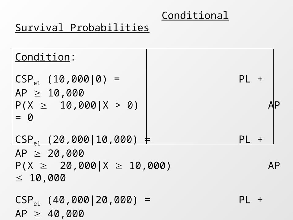
Conditional Survival Probabilities

Condition:

CSPe1 (10,000|0) = PL + AP 10,000P(X 10,000|X > 0) AP = 0

CSPe1 (20,000|10,000) = PL + AP 20,000P(X 20,000|X 10,000) AP 10,000

CSPe1 (40,000|20,000) = PL + AP 40,000P(X 40,000|X 20,000) AP 20,000

AP = Attachment Point PL = Policy Limit X = Gross Loss Amount e1 = empirical lag 1

CSPe1 (10,000|0) = P(X 10,000|X > 0)

Number of occurrences with: Occurrence Size + AP 10,000

Policy limit + AP 10,000 AP = 0

Number of occurrences with: Occurrence Size + AP > 0

Policy limit + AP 10,000 AP = 0

6 (occurrences 3, 6, 7, 9, 10, 11)9 (occurrences 1, 2, 3, 5, 6, 7, 9, 10, 11)

Only occurrences with policy limits plus attachment point greater than or equal to 10,000 are used. Only occurrences with attachment point equal to zero are used.

CSPe1 (20,000|10,000) = P(X 20,000|X 10,000)

Number of occurrences with: Occurrence Size + AP 20,000

Policy limit + AP 20,000 AP 10,000

Number of occurrences with: Occurrence Size + AP > 10,000

Policy limit + AP 20,000 AP 10,000

3 (occurrences 7, 10, 11)6 (occurrences 4, 6, 7, 9, 10, 11)

Only occurrences with policy limits plus attachment point greater than or equal to 20,000 are used. Only occurrences with attachment point less than or equal to 10,000 are used.

CSPe1 (40,000|20,000) = P(X 40,000|X 20,000)

Number of occurrences with: Occurrence Size + AP 40,000

Policy limit + AP 40,000 AP 20,000

Number of occurrences with: Occurrence Size + AP > 20,000

Policy limit + AP 40,000 AP 20,000

1 (occurrence 12)4 (occurrences 8, 10, 11, 12)

Only occurrences with policy limits plus attachment point greater than or equal to 40,000 are used. Only occurrences with attachment point less than or equal to 20,000 are used.

We now calculate the empirical survival probabilities:

Se1 (10,000) = P(X 10,000)

= CSPe1 (10,000|0) = P(X 10,000|X > 0)

= 6/9 = 2/3

Se1 (20,000) = P(X 20,000)

= CSPe1 (10,000|0) * CSPe1 (20,000|10,000)

= P(X 10,000|X > 0) * P(X 20,000|X > 10,000)

= 6/9 * 3/6 = 1/3

Se1 (40,000) = P(X 40,000)

= CSPe1 (10,000|0) * CSPe1 (20,000|10,000) * CSPe1 (40,000|20,000)

= P(X 10,000|X > 0) * P(X 20,000|X > 10,000)

* P(X 40,000|X > 20,000)

= 6/9 * 3/6 * 1/4= 1/12

Lag Weight Calculation

Lag weights are used to combine the survival probabilities

of the lags.

This results in an overall combined empirical survival

probability.

Note: Occurrences from policies with nonzero attachment

points are not used. The weights reflect the lag distribution

of ground-up occurrences and the inclusion of Excess &

Umbrella data might distort the results.

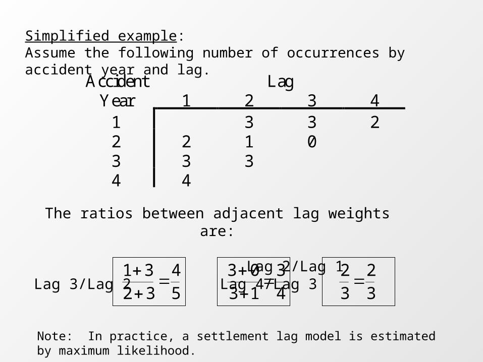
Accident Lag Year 1 2 3 4

1 3 3 2 2 2 1 0

3 3 3

4 4

The ratios between adjacent lag weights are:

Lag 2/Lag 1 Lag 3/Lag 2 Lag 4/Lag 3

Simplified example:Assume the following number of occurrences by accident year and lag.

Note: In practice, a settlement lag model is estimated by maximum likelihood.

54

3231

32

32

43

1303

14

5

1 14

51

4

5

3

41

4

5

3

4

2

3

4

1429

.

14

5

3

4

2

3

1 14

51

4

5

3

41

4

5

3

4

2

3

2

1414

.

1

1 14

51

4

5

3

41

4

5

3

4

2

3

5

1436

.

14

5

3

4

1 14

51

4

5

3

41

4

5

3

4

2

3

3

1421

.

Lag 1:

Lag 4:

Lag 2:

Lag 3:

The Lag Weights Are:

The use of ratios of occurrences between lags avoids distortions that may otherwise result from:

• the shape of the experience period

• accident year exposure growth

Now we combine the empirical survival functions at each lag using the lag weights:

Empirical Survival Function Dollar LagAmount 1 2 3 4 10,000 .67 .80 .85 .90 20,000 .33 .50 .55 .63 40,000 .08 .24 .30 .40

Lag Weights Dollar LagAmount 1 2 3 4 10,000 .36 .29 .21 .14 20,000 .36 .29 .21 .14 40,000 .36 .29 .21 .14

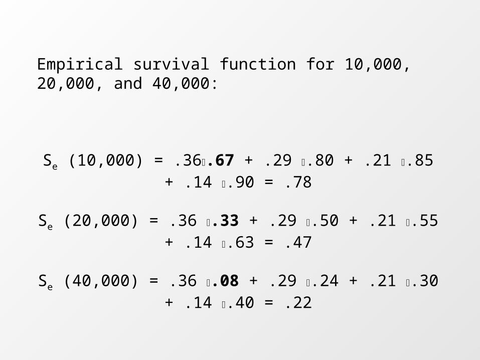
Empirical survival function for 10,000, 20,000, and 40,000:

Se (10,000) = .36.67 + .29 .80 + .21 .85 + .14 .90 = .78

Se (20,000) = .36 .33 + .29 .50 + .21 .55 + .14 .63 = .47

Se (40,000) = .36 .08 + .29 .24 + .21 .30 + .14 .40 = .22

Typical dollar amounts at which the empirical survival function is calculated are:

10 6,000 200,000 5,000,000 25 8,000 250,000 6,000,000 50 10,000 300,000 8,000,000 100 15,000 400,000 10,000,000 250 20,000 500,000 15,000,000 500 25,000 600,000 20,000,0001,000 30,000 800,000 25,000,0001,500 40,000 1,000,000 30,000,0002,000 50,000 1,500,000 40,000,0002,500 60,000 2,000,000 50,000,0003,000 80,000 2,500,000 60,000,0004,000 100,000 3,000,000 80,000,0005,000 150,000 4,000,000 100,000,000

In actual practice:

• The latest five diagonals of data are used.

• Lags n and greater are combined when calculating the empirical survival function since there is no clear difference among them. For General Liability n is 7. For Commercial Automobile Liability n is 5.

• A settlement lag model based on a multinomial distribution is used to include exposure to all settlement lags. An exponential decay assumption implicitly provides nonzero weight at all possible settlement lags.

Fitting a Mixed Exponential Distribution to an Empirical

Distribution

• Once the overall empirical survival function has been calculated at a number of different dollar amounts, a curve may be fit. Maximum likelihood estimation or minimum distance estimation may be used to obtain the fitted mixed exponential parameters.

• The assumption is made that the density function f(x) of the curve should decrease and gradually flatten out as x becomes large. Mathematically speaking, the curve should have alternating derivatives (f(x) > 0, f '(x) < 0, f "(x) > 0, . . .) for all x.

• A theorem proved by S. Bernstein (1928) states that a function has alternating derivatives if and only if it can be written as a mixture of exponential distributions.

• Many common distributions fit to losses either have the alternating derivative property or nearly have the alternating derivative property. The Pareto distribution, in particular, has this property, since it is a mixture of exponential distributions, with the mixing distribution being an inverse gamma distribution.

• The general mixed exponential distribution is extremely flexible, since there are no restrictions on the mixing distribution. In particular, the mixed exponential distribution will provide at least as good a fit as the Pareto distribution or any mixture of Pareto distributions, since the Pareto distribution is a special case of the mixed exponential distribution.

The fitted survival function, based on the mixed exponential distribution, is:

1w 0,m 0, w,ew...ewewS(x) iiim

x-

nm

x-

2m

x-

1n21

- Optimal values of w1, . . . , wn and m1, . . . , mn can be obtained by grouped maximum likelihood estimation or minimum distance estimation. The dollar amounts at which the empirical survival function is calculated serve as the group boundaries (for maximum likelihood estimation) or as the points at which the distance function is evaluated (for minimum distance estimation).

- To obtain the optimal mixed exponential distribution, n is permitted to be as large as necessary. Generally, the optimal distribution is found when n is between 5 and 10. By increasing n above the optimal number, the likelihood function cannot be further increased. Likewise, the distance function cannot be further decreased.

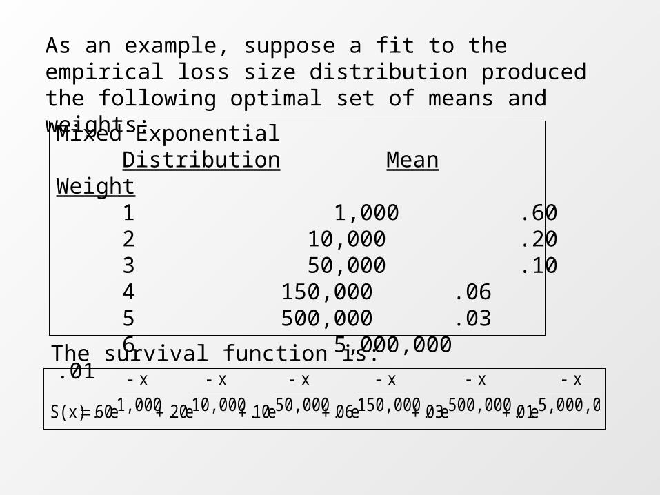
As an example, suppose a fit to the empirical loss size distribution produced the following optimal set of means and weights:

Mixed Exponential Distribution Mean Weight

1 1,000 .602 10,000 .203 50,000 .104 150,000 .065 500,000 .036 5,000,000 .01

The survival function is:

5,000,000

x-

e01.500,000

x-

e03.150,000

x-

e06. 50,000

x-

e10.10,000

x-

e20.1,000

x-

e60.S(x)

The limited average severity (LAS) function is:

LAS(x) =

n

1ii

)Meanx / (i Weight)1(Mean ie

where n equals the number of exponential distributions required.

)10,000

x-

e1(000,1020.)1,000

x-

e1(000,160.LAS(x)

)150,000

x-

e1(000,15006.)50,000

x-

e1(000,5010.+

)5,000,000

x-

e1(000,000,501.)500,000

x-

e1(000,50003.+

n=6 in this example.

Increased limits factors based on this model are as follows:

Policy Limited Average Limit Severity ILF*

100,000 15,012 1.00 300,000 25,049 1.67 500,000 30,519 2.03 1,000,000 38,622 2.57 2,000,000 47,809 3.18 5,000,000 63,205 4.21 10,000,000 74,833 4.98

* Excluding LAE and risk load provisions

Additional Considerations

Other adjustments that must be made as part of the increased limits procedure are:

• Composite rated risk and excess & umbrella data are not segregated by increased limits severity table. A Bayesian allocation is used to distribute each occurrence in a given lag. The relative volume of each table in the lag along with the empirical survival distributions for that lag are used in the allocation.

• Because of the low volume of data in the tail of the distributions, adjustments may be appropriate to ensure stability in the tail for the individual severity tables as well as the relativities between them.

Tail of the Empirical Distribution: An example

To smooth the tail of the empirical distribution:

1. Select a truncation point where the credibility of the empirical survival probabilities becomes low.

2. Over successive intervals just below the truncation point, use percentile matching to examine the indicated parameters of various distributions.

3. Select a distribution which shows stable parameter indications. There should be no parameter trend over this stable region.

4. Use this distribution type, with parameters fit to the stable region, to smooth the empirical distribution beyond the truncation point.

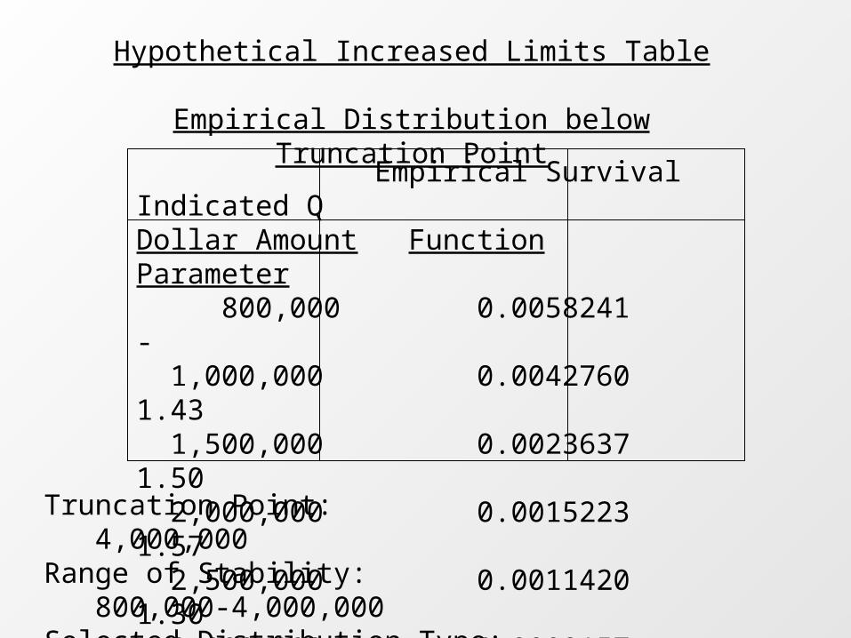
Hypothetical Increased Limits Table

Empirical Distribution below Truncation Point

Empirical Survival Indicated QDollar Amount Function Parameter 800,000 0.0058241 - 1,000,000 0.0042760 1.43 1,500,000 0.0023637 1.50 2,000,000 0.0015223 1.57 2,500,000 0.0011420 1.30 3,000,000 0.0009157 1.22 4,000,000 0.0006274 1.32

Truncation Point: 4,000,000Range of Stability: 800,000-4,000,000Selected Distribution Type: Pareto

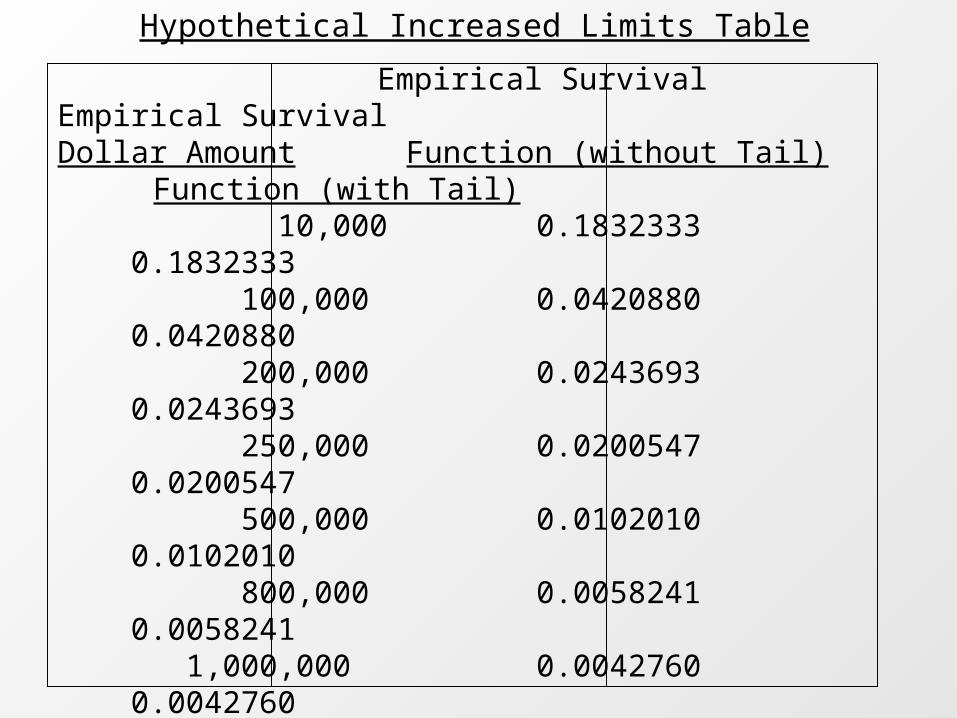
Hypothetical Increased Limits Table

Empirical Survival Empirical SurvivalDollar Amount Function (without Tail) Function (with Tail) 10,000 0.1832333 0.1832333

100,000 0.0420880 0.0420880

200,000 0.0243693 0.0243693

250,000 0.0200547 0.0200547

500,000 0.0102010 0.0102010

800,000 0.0058241 0.0058241

1,000,000 0.0042760 0.0042760

2,500,000 0.0011420 0.0011420

3,000,000 0.0009157 0.0009157

4,000,000 0.0006274 0.0006274

5,000,000 0.0003871 0.0004610

8,000,000 0.0001609 0.0002408

10,000,000 0.0000933 0.0001769

20,000,000 0.0000532 0.0000679

25,000,000 0.0000000 0.0000499

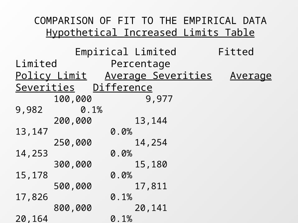
COMPARISON OF FIT TO THE EMPIRICAL DATAHypothetical Increased Limits Table

Empirical Limited Fitted Limited PercentagePolicy Limit Average Severities Average Severities Difference 100,000 9,977 9,982 0.1% 200,000 13,144 13,147 0.0% 250,000 14,254 14,253 0.0% 300,000 15,180 15,178 0.0% 500,000 17,811 17,826 0.1% 800,000 20,141 20,164 0.1% 1,000,000 21,137 21,166 0.1% 1,500,000 22,756 22,744 -0.1% 2,000,000 23,663 23,690 0.1% 2,500,000 24,323 24,352 0.1% 3,000,000 24,837 24,859 0.1% 4,000,000 25,553 25,610 0.2% 5,000,000 26,045 26,147 0.4% 10,000,000 27,088 27,566 1.8%

Current Status of the Mixed Exponential Increased Limits Procedure

• ISO intends to use the new increased limits methodology in its reviews for Commercial Liability Lines in 1999. General Liability has been reviewed and a filing based on this methodology is expected to be made later this year.

• ISO completed a review of Legal Professional Liability using this new methodology. This enabled us to easily include the relatively large amount of deductible data. This review was not filed and is available for separate purchase.

Research using the Mixed Exponential Increased Limits Procedure

ISO is currently reviewing and considering the filing of:

• Other lines of business, including Commercial Automobile Liability and Medical Professional Liability• Separate Premises/Operations Liability tables by state group• A change in increased limits table and state group compositions for Commercial Automobile Liability• A change in the increased limits table class composition for General Liability• A credibility procedure to complement the empirical survival function where necessary

Other Related Research Efforts

• Evaluation of varying ALAE by policy limit• Reevaluation of the current risk load procedure

Further details about the entire mixed exponential increased limits procedure are planned in future ISO Actuarial Services increased limits circulars. In addition, for those who are interested, an updated draft of a paper on the mixed exponential distribution will be available in a few weeks. You may sign up to receive a copy after the session.