Embed Size (px)
Citation preview
2
Basic Definitions and Cutting Tool Geometry, Single Point Cutting Tools
Give us the tools, and we will finish the job. Winston Churchill's message to President Roosevelt
in a radio broadcast on 9 February 1941.
Abstract. This chapter presents the basic terms and their definitions related to he cutting tool geometry according to ISO and AISI standards. It considers the tool geometry and inter-correlation of geometry parameters in three basic systems: tool-in-hand, tool-in-machine, and tool-in-use. It also reveals and resolves the common issues in the selection of geometry parameters including those related to indexable inserts and tool holders. The chapter introduces the concept and basics of advanced representation of cutting tool geometry using vector analysis. A step-by-step approach with self-sufficient coverage of terms, definitions, and rules makes this complicated subject simple as considerations begin with the simplest geometry of a single-point cutting tool and finish with summation of several motions. Extensive exemplification using practical cases enhances understanding of the covered material.
2.1 Basic Terms and Definitions
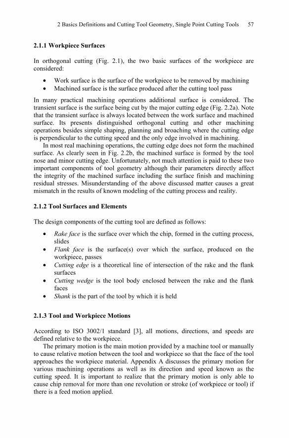
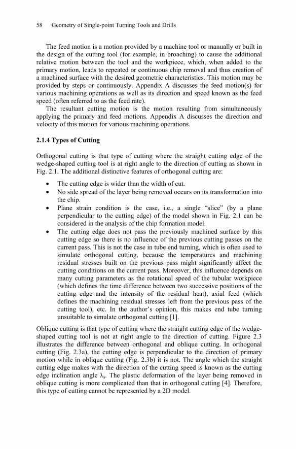
The geometry and nomenclature of cutting tools, even single-point cutting tools, are surprisingly complicated subjects [1]. It is difficult, for example, to determine the appropriate planes in which the various angles of a single-point cutting tool should be measured; it is especially difficult to determine the slope of the tool face. The simplest cutting operation is one in which a straight-edged tool moves with a constant velocity in the direction perpendicular to the cutting edge of the tool. This is known as the two-dimensional or orthogonal cutting process illustrated in Fig. 2.1. The cutting operation can best be understood in terms of orthogonal cutting parameters. Figure 2.2 shows the application of a single-point cutting tool in a turning operation. It helps to correlate the terminology used in orthogonal and oblique non-free cutting.
56 Geometry of Single-point Turning Tools and Drills
Thickness of the layer beingremoved(Uncut chip thickness)
Flank (Relief) angle, α
Rake angle, γ
Chip
Tool
Workpiece
Direction of prime motion(Cutting direction)
wd
t1
Width (depth) of cut(Uncut chip width)
Chip width
dw1 t2
Cutting wedgeCutting edge
Chip thickness
Work surface
Machined surface
Rake angle γ
Tool
Fig. 2.1. Visualization of basic terms in orthogonal cutting (after Astakhov[2])
Direction of prime (speed) motion
Direction of feed motion Tool
Chip
Workpiece
Machined surfaceWork surface Transient surface
Majorcuttingedge
Tool noseradius
AMinorcutting edge
Chip
Cutting insert
Workpiece
SECTION A-A
Machined surface
ENLARGED
A
(a) (b)
Fig. 2.2. Visualization of basic terms in turning: (a) general view and (b) enlarged cutting portion (after Astakhov [2])
This section aims to introduce the basic definitions of the terms and notions involved in tool geometry considerations. Proper definitions and illustrations of these items are important for comprehension of the basic and advanced concept of the tool geometry. This is particularly true because a wide diversity of terms used in the books, texts, research papers, tool companies catalogs, trade materials, and even standards (National and International) combined with the so-called “machine shop terminology” makes it difficult to understand even the basic concepts of the tool geometry.
2 Basics Definitions and Cutting Tool Geometry, Single Point Cutting Tools 57
2.1.1 Workpiece Surfaces
In orthogonal cutting (Fig. 2.1), the two basic surfaces of the workpiece are considered:
• Work surface is the surface of the workpiece to be removed by machining • Machined surface is the surface produced after the cutting tool pass
In many practical machining operations additional surface is considered. The transient surface is the surface being cut by the major cutting edge (Fig. 2.2a). Note that the transient surface is always located between the work surface and machined surface. Its presents distinguished orthogonal cutting and other machining operations besides simple shaping, planning and broaching where the cutting edge is perpendicular to the cutting speed and the only edge involved in machining.
In most real machining operations, the cutting edge does not form the machined surface. As clearly seen in Fig. 2.2b, the machined surface is formed by the tool nose and minor cutting edge. Unfortunately, not much attention is paid to these two important components of tool geometry although their parameters directly affect the integrity of the machined surface including the surface finish and machining residual stresses. Misunderstanding of the above discussed matter causes a great mismatch in the results of known modeling of the cutting process and reality.
2.1.2 Tool Surfaces and Elements
The design components of the cutting tool are defined as follows:
• Rake face is the surface over which the chip, formed in the cutting process, slides
• Flank face is the surface(s) over which the surface, produced on the workpiece, passes
• Cutting edge is a theoretical line of intersection of the rake and the flank surfaces
• Cutting wedge is the tool body enclosed between the rake and the flank faces
• Shank is the part of the tool by which it is held
2.1.3 Tool and Workpiece Motions
According to ISO 3002/1 standard [3], all motions, directions, and speeds are defined relative to the workpiece.
The primary motion is the main motion provided by a machine tool or manually to cause relative motion between the tool and workpiece so that the face of the tool approaches the workpiece material. Appendix A discusses the primary motion for various machining operations as well as its direction and speed known as the cutting speed. It is important to realize that the primary motion is only able to cause chip removal for more than one revolution or stroke (of workpiece or tool) if there is a feed motion applied.
58 Geometry of Single-point Turning Tools and Drills
The feed motion is a motion provided by a machine tool or manually or built in the design of the cutting tool (for example, in broaching) to cause the additional relative motion between the tool and the workpiece, which, when added to the primary motion, leads to repeated or continuous chip removal and thus creation of a machined surface with the desired geometric characteristics. This motion may be provided by steps or continuously. Appendix A discusses the feed motion(s) for various machining operations as well as its direction and speed known as the feed speed (often referred to as the feed rate).
The resultant cutting motion is the motion resulting from simultaneously applying the primary and feed motions. Appendix A discusses the direction and velocity of this motion for various machining operations.
2.1.4 Types of Cutting
Orthogonal cutting is that type of cutting where the straight cutting edge of the wedge-shaped cutting tool is at right angle to the direction of cutting as shown in Fig. 2.1. The additional distinctive features of orthogonal cutting are:
• The cutting edge is wider than the width of cut. • No side spread of the layer being removed occurs on its transformation into
the chip. • Plane strain condition is the case, i.e., a single “slice” (by a plane
perpendicular to the cutting edge) of the model shown in Fig. 2.1 can be considered in the analysis of the chip formation model.
• The cutting edge does not pass the previously machined surface by this cutting edge so there is no influence of the previous cutting passes on the current pass. This is not the case in tube end turning, which is often used to simulate orthogonal cutting, because the temperatures and machining residual stresses built on the previous pass might significantly affect the cutting conditions on the current pass. Moreover, this influence depends on many cutting parameters as the rotational speed of the tubular workpiece (which defines the time difference between two successive positions of the cutting edge and the intensity of the residual heat), axial feed (which defines the machining residual stresses left from the previous pass of the cutting tool), etc. In the author’s opinion, this makes end tube turning unsuitable to simulate orthogonal cutting [1].
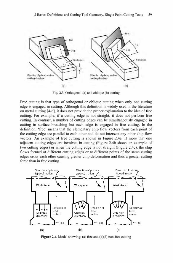
Oblique cutting is that type of cutting where the straight cutting edge of the wedge-shaped cutting tool is not at right angle to the direction of cutting. Figure 2.3 illustrates the difference between orthogonal and oblique cutting. In orthogonal cutting (Fig. 2.3a), the cutting edge is perpendicular to the direction of primary motion while in oblique cutting (Fig. 2.3b) it is not. The angle which the straight cutting edge makes with the direction of the cutting speed is known as the cutting edge inclination angle λs. The plastic deformation of the layer being removed in oblique cutting is more complicated than that in orthogonal cutting [4]. Therefore, this type of cutting cannot be represented by a 2D model.
2 Basics Definitions and Cutting Tool Geometry, Single Point Cutting Tools 59
Fig. 2.3. Orthogonal (a) and oblique (b) cutting
Free cutting is that type of orthogonal or oblique cutting when only one cutting edge is engaged in cutting. Although this definition is widely used in the literature on metal cutting [4-6], it does not provide the proper explanation to the idea of free cutting. For example, if a cutting edge is not straight, it does not perform free cutting. In contrast, a number of cutting edges can be simultaneously engaged in cutting in surface broaching but each edge is engaged in free cutting. In the definition, ‘free’ means that the elementary chip flow vectors from each point of the cutting edge are parallel to each other and do not intersect any other chip flow vectors. An example of free cutting is shown in Figure 2.4a. If more that one adjacent cutting edges are involved in cutting (Figure 2.4b shows an example of two cutting edges) or when the cutting edge is not straight (Figure 2.4c), the chip flows formed at different cutting edges or at different points of the same cutting edges cross each other causing greater chip deformation and thus a greater cutting force than in free cutting.
Figure 2.4. Model showing: (a) free and (c)(d) non-free cutting
60 Geometry of Single-point Turning Tools and Drills
Non-free cutting is that type of cutting where more than one cutting edge is engaged in cutting so that the chip flows from the engaged cutting edges interact with each other (Figure 2.4b,c).
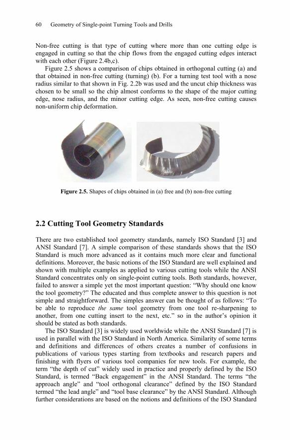
Figure 2.5 shows a comparison of chips obtained in orthogonal cutting (a) and that obtained in non-free cutting (turning) (b). For a turning test tool with a nose radius similar to that shown in Fig. 2.2b was used and the uncut chip thickness was chosen to be small so the chip almost conforms to the shape of the major cutting edge, nose radius, and the minor cutting edge. As seen, non-free cutting causes non-uniform chip deformation.
Figure 2.5. Shapes of chips obtained in (a) free and (b) non-free cutting
2.2 Cutting Tool Geometry Standards
There are two established tool geometry standards, namely ISO Standard [3] and ANSI Standard [7]. A simple comparison of these standards shows that the ISO Standard is much more advanced as it contains much more clear and functional definitions. Moreover, the basic notions of the ISO Standard are well explained and shown with multiple examples as applied to various cutting tools while the ANSI Standard concentrates only on single-point cutting tools. Both standards, however, failed to answer a simple yet the most important question: “Why should one know the tool geometry?” The educated and thus complete answer to this question is not simple and straightforward. The simples answer can be thought of as follows: “To be able to reproduce the same tool geometry from one tool re-sharpening to another, from one cutting insert to the next, etc.” so in the author’s opinion it should be stated as both standards.
The ISO Standard [3] is widely used worldwide while the ANSI Standard [7] is used in parallel with the ISO Standard in North America. Similarity of some terms and definitions and differences of others creates a number of confusions in publications of various types starting from textbooks and research papers and finishing with flyers of various tool companies for new tools. For example, the term “the depth of cut” widely used in practice and properly defined by the ISO Standard, is termed “Back engagement” in the ANSI Standard. The terms “the approach angle” and “tool orthogonal clearance” defined by the ISO Standard termed “the lead angle” and “tool base clearance” by the ANSI Standard. Although further considerations are based on the notions and definitions of the ISO Standard

2 Basics Definitions and Cutting Tool Geometry, Single Point Cutting Tools 61
(with some corrections of some obvious flaws [8]), the basic notions of the ANSI Standard and explanations of the correspondence of the basic terms of both standards are given in further text wherever it is important.
2.3 Systems of Consideration of Tool Geometry
Both the above-mentioned tool geometry standards discuss two systems of consideration of the cutting tool geometry, namely, the tool-in-hand and tool-in-use systems (hereafter, T-hand-S and T-use-S, respectively). The former relates to the so-called static geometry while the latter is based on consideration of tool motions with respect to the workpiece. In the author’s opinion, however, these two systems are insufficient for the proper consideration of cutting tool geometry. Another system, namely, the tool-in-machine system [1] (hereafter, T-mach-S) should also be considered.
Introduction of an additional system of consideration may be thought of as a kind of overcomplicating of the cutting tool geometry and its practical applications so that it is suitable only for ivory academicians as it has little practical value at the shop floor level. In the author’s opinion, the opposite is actually the case. Namely, misunderstanding the tool geometry in the above-mentioned system leads to improper selection of the tool geometry parameters and humps optimization of practical machining operations. Moreover, tool life and quality of the machined surface are often not as good as they could be if the tool geometry were selected properly. In other words, the proposed consideration does not complicate but rather simplifies the analysis of tool geometry.
The cutting tool geometry includes a number of angles measured in different planes. Although the definitions of the standard planes for consideration of tool geometry are the same for all of the three above-mentioned systems of consideration, these planes are not the same in these systems. This is because a set of the standard planes in each particular system is defined in a certain coordinate system. Thus, it is of crucial importance to set the proper coordinate system in each system of consideration. Such a coordinate system distinguishes one system under consideration from others within the three basic systems of consideration. Note that if the coordinate systems of two or more systems of consideration coincide then there is no need to consider these systems separately as the set of the reference planes would be the same.
The choice of a particular system and/or their combinations depends on the tool and toolholder design, tool post, and tool fixing in the machine, direction of the tool motion with respect to the workpiece or axis of rotation and other factors. Such a choice, however, should always have a clear objective, namely, to be correlated in simple fashion to the cutting tool geometry needed for optimum tool performance. In the case of a cutting tool with indexable inserts, the objective is to select the proper inserts and available tool holder to assure the tool geometry required by the optimal performance of the machining operation. Therefore, the starting point of tool design (selection) is the optimum cutting geometry and the finishing point is the tool grinding geometry or specifically selected tool holders and inserts to assure this optimal cutting geometry. To do this, a tool designer (tool
62 Geometry of Single-point Turning Tools and Drills
layout, tool application and tool optimization specialists, manufacturing and process engineers) should know the basic definitions and parameters of tool geometry, the above-mentioned three systems of consideration of tool geometry, as well as the correlations among these systems. One of the prime objectives of this book is to introduce these items showing their practical implementation in single point and in drilling tools with multiple real-world examples.
Being simple, logical, and straightforward, the above-stated representation of the tool geometry is not common while being indirectly used for years in various books and research papers. Therefore, a simple exemplification can clarify the essence of the proposed three systems.
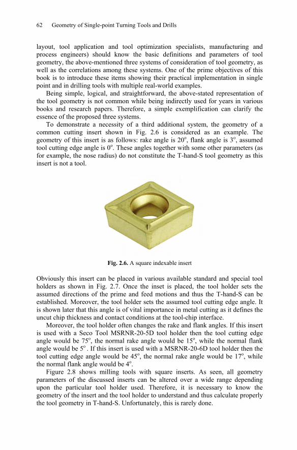
To demonstrate a necessity of a third additional system, the geometry of a common cutting insert shown in Fig. 2.6 is considered as an example. The geometry of this insert is as follows: rake angle is 20o, flank angle is 3o, assumed tool cutting edge angle is 0o. These angles together with some other parameters (as for example, the nose radius) do not constitute the T-hand-S tool geometry as this insert is not a tool.
Fig. 2.6. A square indexable insert
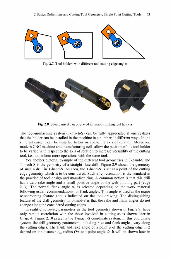
Obviously this insert can be placed in various available standard and special tool holders as shown in Fig. 2.7. Once the inset is placed, the tool holder sets the assumed directions of the prime and feed motions and thus the T-hand-S can be established. Moreover, the tool holder sets the assumed tool cutting edge angle. It is shown later that this angle is of vital importance in metal cutting as it defines the uncut chip thickness and contact conditions at the tool-chip interface.
Moreover, the tool holder often changes the rake and flank angles. If this insert is used with a Seco Tool MSRNR-20-5D tool holder then the tool cutting edge angle would be 75o, the normal rake angle would be 15o, while the normal flank angle would be 5o . If this insert is used with a MSRNR-20-6D tool holder then the tool cutting edge angle would be 45o, the normal rake angle would be 17o, while the normal flank angle would be 4o.
Figure 2.8 shows milling tools with square inserts. As seen, all geometry parameters of the discussed inserts can be altered over a wide range depending upon the particular tool holder used. Therefore, it is necessary to know the geometry of the insert and the tool holder to understand and thus calculate properly the tool geometry in T-hand-S. Unfortunately, this is rarely done.
2 Basics Definitions and Cutting Tool Geometry, Single Point Cutting Tools 63
Fig. 2.7. Tool holders with different tool cutting edge angles
Fig. 2.8. Square insert can be placed in various milling tool holders
The tool-in-machine system (T-mach-S) can be fully appreciated if one realizes that the holder can be installed in the machine in a number of different ways. In the simplest case, it can be installed below or above the axis of rotation. Moreover, modern CNC machine and manufacturing cells allow the position of the tool holder to be varied with respect to the axis of rotation to increase versatility of the cutting tool, i.e., to perform more operations with the same tool.
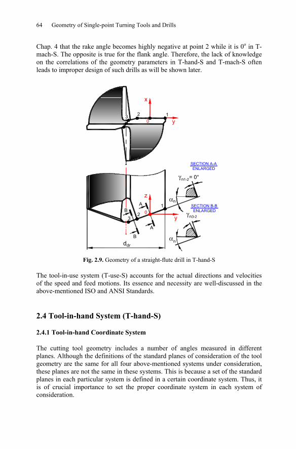
Yes another pictorial example of the different tool geometries in T-hand-S and T-mach-S is the geometry of a straight-flute drill. Figure 2.9 shows the geometry of such a drill in T-hand-S. As seen, the T-hand-S is set at a point of the cutting edge geometry which is to be considered. Such a representation is the standard in the practice of tool design and manufacturing. A common notion is that this drill has a zero rake angle and a small positive angle of the web-thinning part (edge 2−3). The normal flank angle αn is selected depending on the work material following usual recommendations for flank angles. This angle is used as the major re-sharpening feature and is indicated on the tool drawing. The distinguishing feature of the drill geometry in T-hand-S is that the rake and flank angles do not change along the considered cutting edges.
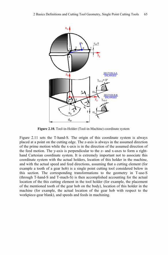
In reality, however, parameters as the tool geometry shown in Fig. 2.9, have only remote correlation with the those involved in cutting as is shown later in Chap. 4. Figure 2.10 presents the T-mach-S coordinate system. In this coordinate system, the drill geometry parameters, including rake and flank angles, vary along the cutting edges. The flank and rake angle of a point a of the cutting edge 1−2 depend on the distance cct, radius Oa, and point angle Φ. It will be shown later in
64 Geometry of Single-point Turning Tools and Drills
Chap. 4 that the rake angle becomes highly negative at point 2 while it is 0o in T-mach-S. The opposite is true for the flank angle. Therefore, the lack of knowledge on the correlations of the geometry parameters in T-hand-S and T-mach-S often leads to improper design of such drills as will be shown later.
12y
x
0
23
1A
A
B
B
0
z
y
3
n1-2γ = 0°
αn
αn
γn3-2ENLARGED
SECTION B-B
ENLARGEDSECTION A-A
ddr
Fig. 2.9. Geometry of a straight-flute drill in T-hand-S
The tool-in-use system (T-use-S) accounts for the actual directions and velocities of the speed and feed motions. Its essence and necessity are well-discussed in the above-mentioned ISO and ANSI Standards.
2.4 Tool-in-hand System (T-hand-S)
2.4.1 Tool-in-hand Coordinate System
The cutting tool geometry includes a number of angles measured in different planes. Although the definitions of the standard planes of consideration of the tool geometry are the same for all four above-mentioned systems under consideration, these planes are not the same in these systems. This is because a set of the standard planes in each particular system is defined in a certain coordinate system. Thus, it is of crucial importance to set the proper coordinate system in each system of consideration.
2 Basics Definitions and Cutting Tool Geometry, Single Point Cutting Tools 65
12
y
x
ddr
z
ctc /2
0
23
1
pΦ
κr
f
A
AB
B
0
0
0
y0
0
4
3 a
va
γn3-2
n
ENLARGEDSECTION A-A
αn
ENLARGEDSECTION B-B
n1-2γ = 0°
α
Figure 2.10. Tool-in-Holder (Tool-in-Machine) coordinate system
Figure 2.11 sets the T-hand-S. The origin of this coordinate system is always placed at a point on the cutting edge. The z-axis is always in the assumed direction of the prime motion while the x-axis is in the direction of the assumed direction of the feed motion. The y-axis is perpendicular to the z- and x-axes to form a right-hand Cartesian coordinate system. It is extremely important not to associate this coordinate system with the actual holders, location of this holder in the machine, and with the actual speed and feed directions, assuming that a cutting element (for example a tooth of a gear hob) is a single point cutting tool considered below in this section. The corresponding transformations to the geometry in T-use-S (through T-hand-S and T-mach-S) is then accomplished accounting for the actual location of the this cutting element in the tool holder (for example, the placement of the mentioned tooth of the gear hob on the body), location of this holder in the machine (for example, the actual location of the gear hob with respect to the workpiece-gear blank), and speeds and feeds in machining.
66 Geometry of Single-point Turning Tools and Drills
vf
vf
x
y
z
κr
Pr
1'
3'
2'
3 1
2
κ r1
Main Reference Plane
PAssumed WorkingPlane
f
v
3
2
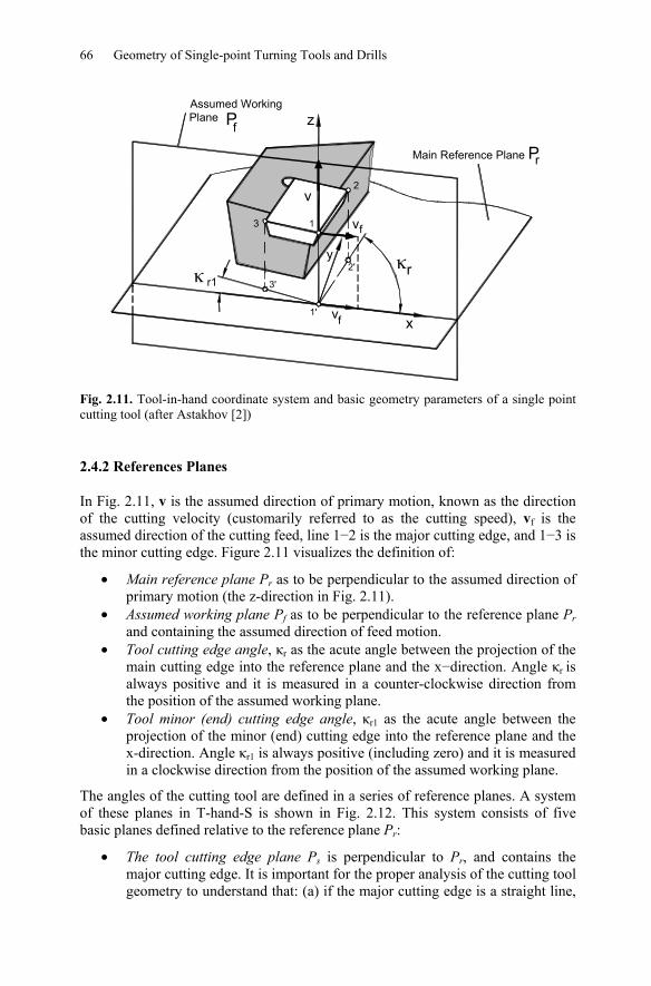
Fig. 2.11. Tool-in-hand coordinate system and basic geometry parameters of a single point cutting tool (after Astakhov [2])
2.4.2 References Planes
In Fig. 2.11, v is the assumed direction of primary motion, known as the direction of the cutting velocity (customarily referred to as the cutting speed), vf is the assumed direction of the cutting feed, line 1−2 is the major cutting edge, and 1−3 is the minor cutting edge. Figure 2.11 visualizes the definition of:
• Main reference plane Pr as to be perpendicular to the assumed direction of primary motion (the z-direction in Fig. 2.11).
• Assumed working plane Pf as to be perpendicular to the reference plane Pr and containing the assumed direction of feed motion.
• Tool cutting edge angle, κr as the acute angle between the projection of the main cutting edge into the reference plane and the x−direction. Angle κr is always positive and it is measured in a counter-clockwise direction from the position of the assumed working plane.
• Tool minor (end) cutting edge angle, κr1 as the acute angle between the projection of the minor (end) cutting edge into the reference plane and the x-direction. Angle κr1 is always positive (including zero) and it is measured in a clockwise direction from the position of the assumed working plane.
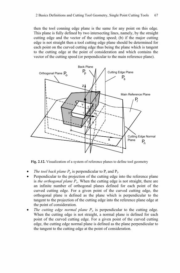
The angles of the cutting tool are defined in a series of reference planes. A system of these planes in T-hand-S is shown in Fig. 2.12. This system consists of five basic planes defined relative to the reference plane Pr:
• The tool cutting edge plane Ps is perpendicular to Pr, and contains the major cutting edge. It is important for the proper analysis of the cutting tool geometry to understand that: (a) if the major cutting edge is a straight line,
2 Basics Definitions and Cutting Tool Geometry, Single Point Cutting Tools 67
then the tool conning edge plane is the same for any point on this edge. This plane is fully defined by two intersecting lines, namely, by the straight cutting edge and the vector of the cutting speed; (b) if the major cutting edge is not straight then a tool cutting edge plane should be determined for each point on the curved cutting edge thus being the plane which is tangent to the cutting edge at the point of consideration and which contains the vector of the cutting speed (or perpendicular to the main reference plane).
vf
x
y
z
Pr
3 1
2
Main Reference Plane
0
Cutting Edge Plane
Ps
Back Plane
Po
Cutting Edge NormalPlane Pn
Orthogonal Plane pP
3
v
Fig. 2.12. Visualization of a system of reference planes to define tool geometry
• The tool back plane Pp is perpendicular to Pr and Pf. • Perpendicular to the projection of the cutting edge into the reference plane
is the orthogonal plane Po. When the cutting edge is not straight, there are an infinite number of orthogonal planes defined for each point of the curved cutting edge. For a given point of the curved cutting edge, the orthogonal plane is defined as the plane which is perpendicular to the tangent to the projection of the cutting edge into the reference plane edge at the point of consideration.
• The cutting edge normal plane Pn is perpendicular to the cutting edge. When the cutting edge is not straight, a normal plane is defined for each point of the curved cutting edge. For a given point of the curved cutting edge, the cutting edge normal plane is defined as the plane perpendicular to the tangent to the cutting edge at the point of consideration.
68 Geometry of Single-point Turning Tools and Drills
2.4.3 Tool Angles
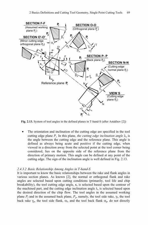
2.4.3.1 Definitions The geometry of a cutting element is defined by certain basic tool angles and thus precise definitions of these angles are essential. A system of tool angles is shown in Fig. 2.13 and is known as the tool-in-hand system (T-hand-S) [1]. Rake, wedge, and flank angles are designated by γ, β, and α, respectively, and these are further identified by the subscript of the plane of consideration. The definitions of basic tool angles in the T-hand-S are as follows:
• ψr is the tool approach angle; it is the acute angle that Ps makes with Pp and is measured in the reference plane Pr as shown in Fig. 2.13.
• The rake angles are defined in the corresponding planes of measurement. The rake angle is the angle between the reference plane (the trace of which in the considered plane of measurement appears as the normal to the direction of primary motion) and the intersection line formed by the considered plane of measurement and the tool rake face. The rake angle is defined as always being acute when looking across the rake face from the selected point and along the line of intersection of the face and plane of measurement. The viewed line of intersection lies on the opposite side of the tool reference plane from the direction of primary motion in the measurement plane for γf, γp, γo, or a major component of it appears in the normal plane for γn. Angle γf is known as the tool side rake, γp is known as the tool back rake, and γn is know is the normal rake. The sign of the rake angles is well defined (Fig. 2.13).
• The flank angles are defined in a similar way to the rake angles, though here if the viewed line of intersection lies on the opposite side of the cutting edge plane Ps from the direction of feed motion, assumed or actual as the case may be, then the flank angle is positive. The flank (sometimes referred to as the clearance) angle is the angle between the tool cutting edge plane Ps and the intersection line formed by the tool flank plane and the considered plane of measurement as shown in Fig. 2.13. Angles αf, αp, αo, αn are clearly defined in the corresponding planes as seen in Fig. 2.13. Angle αf is known as the tool side flank, αp is known as the tool back flank, and αn is know is the normal flank.
• The wedge angles βf, βp, βo, βn are defined in the planes of measurements. The wedge angle is the angle between the two intersection lines formed as the corresponding plane of measurement intersects with the rake and flank faces. For all cases, the sum of the rake, wedge and clearance angles is 90o, i.e.
90op p p n n n o o o f f fγ β α γ β α γ β α γ β α+ + = + + = + + = + + = (2.1)
2 Basics Definitions and Cutting Tool Geometry, Single Point Cutting Tools 69
αn
nβ
γn
λ s
−λ
+λ
pα
βpp
γ
N
N
αoβo
γo
FO
P
P
F
O
αf
fγ
βf
S
−γ
+γ
κr
ψr
κr12
01
3
O'
1oα
O'
(Assumed working plane P )
SECTION F-F
f
P(Orthogonal plane P )
SECTION O-Oo
SECTION O'-O'
(Back plane P )SECTION P- P
p
(Cutting edgenormal plane P )
SECTION N-N
n
(Minor cutting edgeorthogonal plane P )o'
r
PpPr
Pf
Pr
Ps
Ps
Reference plane Pr
(Cutting edgeplane P )
VIEW S
s
Pr Fig. 2.13. System of tool angles in the defined planes in T-hand-S (after Astakhov [2])
• The orientation and inclination of the cutting edge are specified in the tool cutting edge plane Ps. In this plane, the cutting edge inclination angle λs is the angle between the cutting edge and the reference plane. This angle is defined as always being acute and positive if the cutting edge, when viewed in a direction away from the selected point at the tool corner being considered, lies on the opposite side of the reference plane from the direction of primary motion. This angle can be defined at any point of the cutting edge. The sign of the inclination angle is well defined in Fig. 2.13.
2.4.3.2 Basic Relationship Among Angles in T-hand-S It is important to know the basic relationships between the rake and flank angles in various section planes. As known [2], the normal or orthogonal flank and rake angles are selected based upon cutting conditions (primarily, tool life and chip breakability), the tool cutting edge angle, κr is selected based upon the contour of the machined part, and the cutting edge inclination angle λs is selected based upon the desired direction of the chip flow. The tool angles in the assumed working plane Pf and in the assumed back plane, Pp, namely, the tool side rake, γf, the tool back rake γp, the tool side flank, αf, and the tool back flank αp, do not directly
70 Geometry of Single-point Turning Tools and Drills
affect the cutting process. Rather, they serve some useful purposes in the tool manufacturing (assembly) and in preventing tool interference with the workpiece.
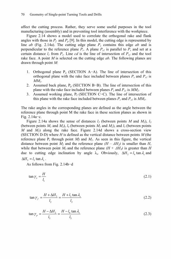
Figure 2.14 shows a model used to correlate the orthogonal rake and flank angles with those in Pf and Pp [9]. In this model, the cutting edge is represented by line ab (Fig. 2.14a). The cutting edge plane Ps contains this edge ab and is perpendicular to the reference plane Pr. A plane Ps1 is parallel to Ps and set at a certain distance l1 from Ps. Line cd is the line of intersection of Ps1 and the tool rake face. A point M is selected on the cutting edge ab. The following planes are drawn through point M:
1. Orthogonal plane Po (SECTION A−A). The line of intersection of this orthogonal plane with the rake face included between planes Ps and Ps1 is MM1.
2. Assumed back plane, Pp (SECTION B−B). The line of intersection of this plane with the rake face included between planes Ps and Ps1 is MM2.
3. Assumed working plane, Pf (SECTION C−C). The line of intersection of this plane with the rake face included between planes Ps and Ps1 is MM3.
The rake angles in the corresponding planes are defined as the angle between the reference plane through point M the rake face in these section planes as shown in Fig. 2.14a−c.
Figure 2.14a shows the sense of distances l2 (between points M and M3), l3 (between points M1 and M3), l4 (between points M1 and M2), and l5 (between points M and M2) along the rake face. Figure 2.14d shows a cross-section view (SECTION D-D) where H is defined as the vertical distance between points M (the reference plane Pr through point M) and M1. As seen in this figure, the vertical distance between point M2 and the reference plane (H – ΔH2) is smaller than H, while that between point M3 and the reference plane (H + ΔH3) is greater than H due to cutting edge inclination by angle λs. Obviously, 2 4 tan sH l λΔ = and
3 3 tan sH l λΔ = . As follows from Fig. 2.14b−d
1
tan oHl
γ = (2.1)
3 3
2 2
tantan s
fH H H l
l lλγ + Δ +
= = (2.2)
42
5 5
tantan s
pH lH H
l lλγ −− Δ
= = (2.3)
2 Basics Definitions and Cutting Tool Geometry, Single Point Cutting Tools 71
c
b
M
a
d
M
l
l
l
l
l
κ 1
M2
M3 3
4
5
2
1
r
κr
y
x
a
bMM
z
M2M1 M3
M
z
ΔHH
-ΔH
H λ
λ
M2
22
M1 M3
H
l3l4
H-Δ
H3
ΔH3
B B
C
C
A
D
DA
H0
l1 l 5 l2
α oα p
α f
M
c
d
α o αp
α f
H-Δ
H2
H-ΔH3
SECTION A-AENLRG. & ROT.
H
SECTION B-BENLRG. & ROT.
SECTION C-CENLRG. & ROT.
SECTION D-DENLRG. & ROT.
κr Pp
Ps1PsPf
PoPr
(a) (e)
(d)(c)(b)
s
s
Fig. 2.14. Model to correlate the orthogonal rake and flank angles with those in the working and back planes
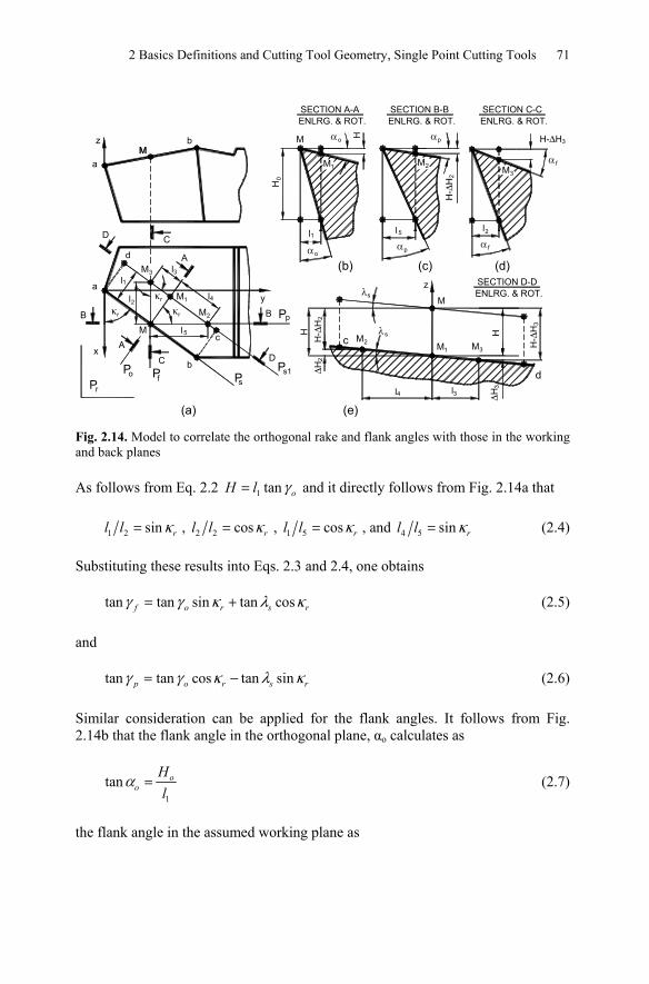
As follows from Eq. 2.2 1 tan oH l γ= and it directly follows from Fig. 2.14a that
1 2 sin rl l κ= , 2 2 cos rl l κ= , 1 5 cos rl l κ= , and 4 5 sin rl l κ= (2.4)
Substituting these results into Eqs. 2.3 and 2.4, one obtains
tan tan sin tan cosf o r s rγ γ κ λ κ= + (2.5)
and
tan tan cos tan sinp o r s rγ γ κ λ κ= − (2.6)
Similar consideration can be applied for the flank angles. It follows from Fig. 2.14b that the flank angle in the orthogonal plane, αo calculates as
1
tan oo
Hl
α = (2.7)
the flank angle in the assumed working plane as
72 Geometry of Single-point Turning Tools and Drills
2
tan of
Hl
α = (2.8)
and the flank angle in the assumed working plane as
5
tan op
Hl
α = (2.9)
It follows from Eq. 2.8 that 1 tano oH l α= . Substituting this results into Eqs. 2.9 and 2.10 and accounting for Eq. 2.5, one can obtain
tan tan sinf o rα α κ= (2.10)
and
tan tan cosp o rα α κ= (2.11)
Although the model shown in Fig. 2.14 is constructed assuming positive rake and inclination angles, the results obtained are also valid for negative rake and/or inclination angles provided that these angles are substituted into the resulting Eqs. 2.6 and 2.7 with the corresponding signs.
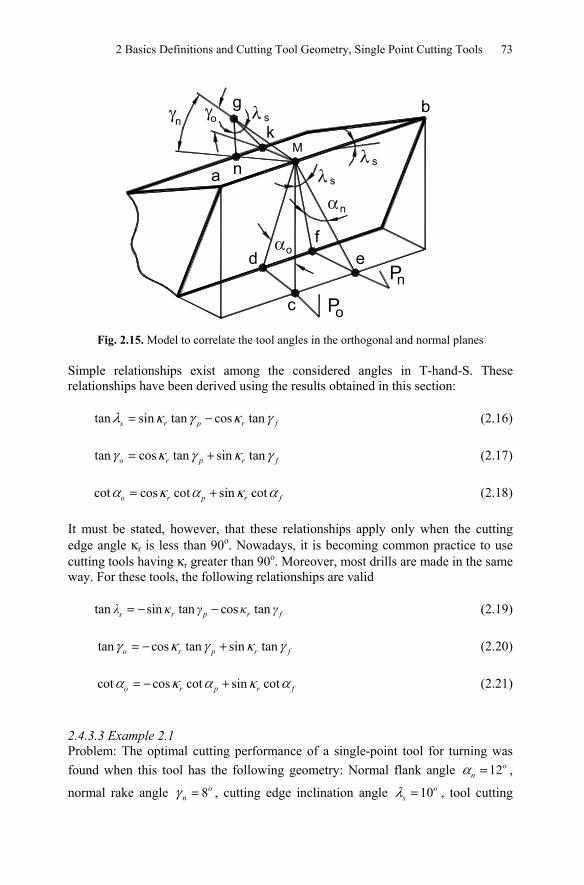
Figure 2.15 shows a model that helps to correlate the tool angles in the orthogonal, Po and in the normal, Pn planes. The cutting edge ab provided with the rake and flank angles is inclined at angle λs. The orthogonal rake, γo and flank, αo angles are considered in the orthogonal plane, Po while the normal rake, γn and flank, αn angles are considered in the orthogonal plane, Pn. As seen
tan o dc Mcα = and tan n fe Meα = (2.12)
As dc fe= and cos sMc Me λ= ⋅ , one can obtain
cot cos cotn s oα λ α= (2.13)
Similarly,
tan o gk Mgγ = and tan n ng Mgγ = (2.14)
As cos ,sgk ng λ= one can obtain
tan cos tann s oγ λ γ= (2.15)
2 Basics Definitions and Cutting Tool Geometry, Single Point Cutting Tools 73
M
a
bg
k
n
d
c
efαo
α n
λ
γoγn
s
λ s
λ s
Po
Pn
Fig. 2.15. Model to correlate the tool angles in the orthogonal and normal planes
Simple relationships exist among the considered angles in T-hand-S. These relationships have been derived using the results obtained in this section:
tan sin tan cos tans r p r fλ κ γ κ γ= − (2.16)
tan cos tan sin tano r p r fγ κ γ κ γ= + (2.17)
cot cos cot sin coto r p r fα κ α κ α= + (2.18)
It must be stated, however, that these relationships apply only when the cutting edge angle κr is less than 90o. Nowadays, it is becoming common practice to use cutting tools having κr greater than 90o. Moreover, most drills are made in the same way. For these tools, the following relationships are valid
tan sin tan cos tans r p r fλ κ γ κ γ= − − (2.19)
tan cos tan sin tano r p r fγ κ γ κ γ= − + (2.20)
cot cos cot sin coto r p r fα κ α κ α= − + (2.21)
2.4.3.3 Example 2.1 Problem: The optimal cutting performance of a single-point tool for turning was found when this tool has the following geometry: Normal flank angle 12o
nα = ,
normal rake angle 8onγ = , cutting edge inclination angle 10o
sλ = , tool cutting
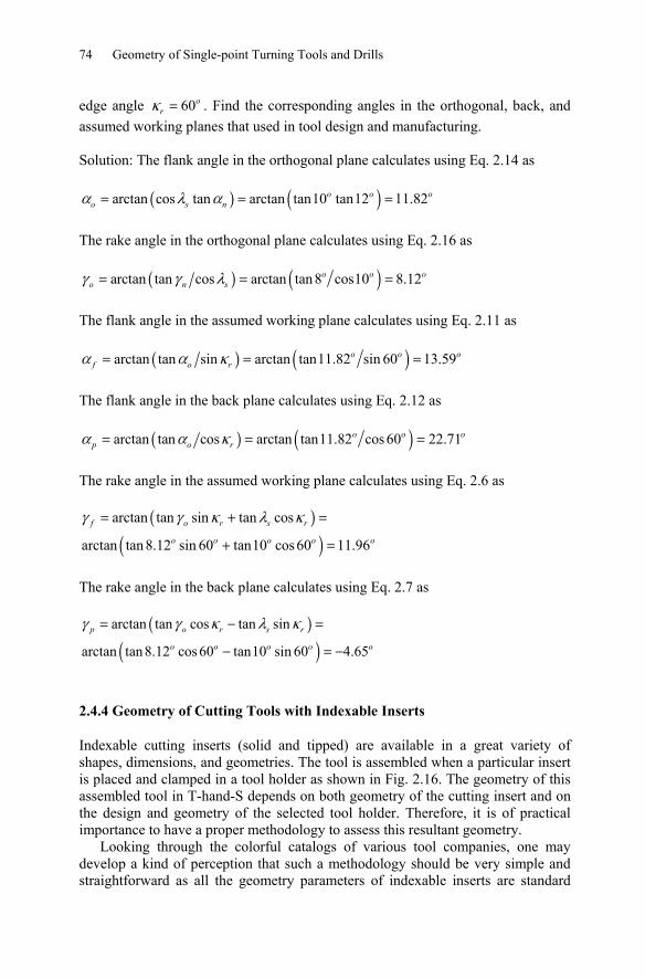
74 Geometry of Single-point Turning Tools and Drills
edge angle 60orκ = . Find the corresponding angles in the orthogonal, back, and
assumed working planes that used in tool design and manufacturing. Solution: The flank angle in the orthogonal plane calculates using Eq. 2.14 as
( ) ( )arctan cos tan arctan tan10 tan12 11.82o o oo s nα λ α= = =
The rake angle in the orthogonal plane calculates using Eq. 2.16 as
( ) ( )arctan tan cos arctan tan8 cos10 8.12o o oo n sγ γ λ= = =
The flank angle in the assumed working plane calculates using Eq. 2.11 as
( ) ( )arctan tan sin arctan tan11.82 sin 60 13.59o o of o rα α κ= = =
The flank angle in the back plane calculates using Eq. 2.12 as
( ) ( )arctan tan cos arctan tan11.82 cos 60 22.71o o op o rα α κ= = =
The rake angle in the assumed working plane calculates using Eq. 2.6 as
( )( )
arctan tan sin tan cos
arctan tan 8.12 sin 60 tan10 cos 60 11.96f o r s r
o o o o o
γ γ κ λ κ= + =
+ =
The rake angle in the back plane calculates using Eq. 2.7 as
( )( )
arctan tan cos tan sin
arctan tan8.12 cos 60 tan10 sin 60 4.65p o r s r
o o o o o
γ γ κ λ κ= − =
− = −
2.4.4 Geometry of Cutting Tools with Indexable Inserts
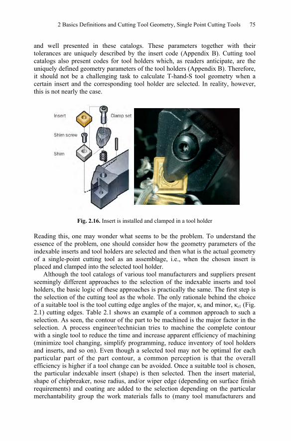
Indexable cutting inserts (solid and tipped) are available in a great variety of shapes, dimensions, and geometries. The tool is assembled when a particular insert is placed and clamped in a tool holder as shown in Fig. 2.16. The geometry of this assembled tool in T-hand-S depends on both geometry of the cutting insert and on the design and geometry of the selected tool holder. Therefore, it is of practical importance to have a proper methodology to assess this resultant geometry.
Looking through the colorful catalogs of various tool companies, one may develop a kind of perception that such a methodology should be very simple and straightforward as all the geometry parameters of indexable inserts are standard
2 Basics Definitions and Cutting Tool Geometry, Single Point Cutting Tools 75
and well presented in these catalogs. These parameters together with their tolerances are uniquely described by the insert code (Appendix B). Cutting tool catalogs also present codes for tool holders which, as readers anticipate, are the uniquely defined geometry parameters of the tool holders (Appendix B). Therefore, it should not be a challenging task to calculate T-hand-S tool geometry when a certain insert and the corresponding tool holder are selected. In reality, however, this is not nearly the case.
Fig. 2.16. Insert is installed and clamped in a tool holder
Reading this, one may wonder what seems to be the problem. To understand the essence of the problem, one should consider how the geometry parameters of the indexable inserts and tool holders are selected and then what is the actual geometry of a single-point cutting tool as an assemblage, i.e., when the chosen insert is placed and clamped into the selected tool holder.
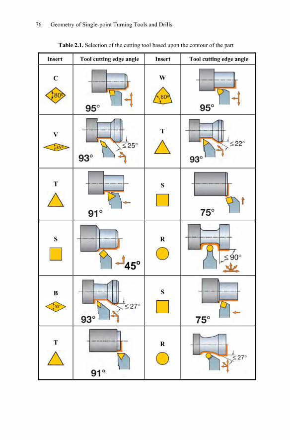
Although the tool catalogs of various tool manufacturers and suppliers present seemingly different approaches to the selection of the indexable inserts and tool holders, the basic logic of these approaches is practically the same. The first step is the selection of the cutting tool as the whole. The only rationale behind the choice of a suitable tool is the tool cutting edge angles of the major, κr and minor, κr1 (Fig. 2.1) cutting edges. Table 2.1 shows an example of a common approach to such a selection. As seen, the contour of the part to be machined is the major factor in the selection. A process engineer/technician tries to machine the complete contour with a single tool to reduce the time and increase apparent efficiency of machining (minimize tool changing, simplify programming, reduce inventory of tool holders and inserts, and so on). Even though a selected tool may not be optimal for each particular part of the part contour, a common perception is that the overall efficiency is higher if a tool change can be avoided. Once a suitable tool is chosen, the particular indexable insert (shape) is then selected. Then the insert material, shape of chipbreaker, nose radius, and/or wiper edge (depending on surface finish requirements) and coating are added to the selection depending on the particular merchantability group the work materials falls to (many tool manufacturers and
76 Geometry of Single-point Turning Tools and Drills
Table 2.1. Selection of the cutting tool based upon the contour of the part
Insert Tool cutting edge angle Insert Tool cutting edge angle
C
W
V
T
T
S
S
45o
R
B
S
T
R
2 Basics Definitions and Cutting Tool Geometry, Single Point Cutting Tools 77
suppliers provide their own classification of work materials). Once the insert is finalized, a suitable tool holder to accommodate this insert is then selected.
Note that in the selection process, the tool rake and flank angles are not considered. One may wonder if there is any way to know these angles after the tool is assembled.
2.4.4.1 Geometry Parameters of Indexable Inserts Appendix B presents the classification of the indexable and tipped cutting inserts according to ANSI and ISO standards. The following parameters of the cutting tool geometry are distinguished by these standards:
• The shape of inserts (Tables B.1 and B.12). This may give only a very vague idea of the tool cutting edge angle because this angle is mainly determined by the tool holder. However, the shape of insert indicates a possible range of the tool cutting edge angle and the tool cutting edge angle of the minor cutting edge variations which is the starting point in the selection of a particular shape. For an insert with a wiper cutting edge, however, the tool cutting edge angle of the major and minor cutting edges are clearly indicated as follows from Tables B.7 and B.20.
• Flank angle. There are eight possible flank angles of standard inserts as follows from Tables B.2 and B.13. Clearly cutting is not possible with a zero clearance angle (N) so the holder must provide a certain flank angle needed in practical machining operations. To provide this flank angle, the insert is tilted in the holder so that the rake face becomes “negative” and thus the clearance along the cutting edge is assured. Needless to say, indexable inserts with zero flank angle (N) are the most popular in practice because both sides of the insert can be used, i.e., the number of useful corners doubles. However, this advantage can only be gained if the tool holder is selected properly to provide the optimal flank angle.
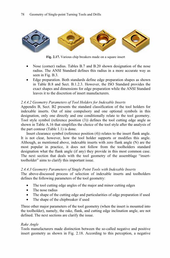
• Rake angle. This angle is not specified by both standards. Therefore, the words “negative”/”positive” inserts do not have rationale behind them and are thus conditional for indexable inserts with chipbreakes. As seen in Tables B.4 and B.17, inserts are available with flat faces or with a chipbreaker made on one or both rake faces. Although this will be discussed later in the consideration of the influence of the rake angle on the cutting process and its outcome, it is worth mentioning here that an indexable insert of the same shape, size, tolerance, etc. can be made with considerably different chip breakers as shown in Fig. 2.17. It is understood that the rake angle and chip deformation is not the same for all shown inserts.
78 Geometry of Single-point Turning Tools and Drills
Fig. 2.17. Various chip breakers made on a square insert
• Nose (corner) radius. Tables B.7 and B.20 shown designation of the nose radius. The ANSI Standard defines this radius in a more accurate way as seen in Fig. B.3.
• Edge preparation. Both standards define edge preparation shapes as shown in Table B.8 and Sect. B.1.2.3. However, the ISO Standard provides the exact shapes and dimensions for edge preparation while the ANSI Standard leaves it to the discretion of insert manufacturers.
2.4.4.2 Geometry Parameters of Tool Holders for Indexable Inserts Appendix B, Sect. B2 presents the standard classification of the tool holders for indexable inserts. Out of nine compulsory and one optional symbols in this designation, only one directly and one conditionally relate to the tool geometry. Tool style symbol (reference position (3)) defines the tool cutting edge angle as shown in Table A.16 that simplifies the choice of the tool style after the analysis of the part contour (Table 1.1) is done.
Insert clearance symbol (reference position (4)) relates to the insert flank angle. It is not clear, however, how the tool holder supports or modifies this angle. Although, as mentioned above, indexable inserts with zero flank angle (N) are the most popular in practice, it does not follow from the toolholders standard designation what the flank angle (if any) they provide in this most common case. The next section that deals with the tool geometry of the assemblage “insert-toolholder” aims to clarify this important issue.
2.4.4.3 Geometry Parameters of Single Point Tools with Indexable Inserts The above-discussed process of selection of indexable inserts and toolholders defines the following parameters of the tool geometry:
• The tool cutting edge angles of the major and minor cutting edges • The nose radius • The shape of the cutting edge and particularities of edge preparation if used • The shape of the chipbreaker if used
Three other major parameters of the tool geometry (when the insert is mounted into the toolholder), namely, the rake, flank, and cutting edge inclination angle, are not defined. The next sections are clarify the issue.
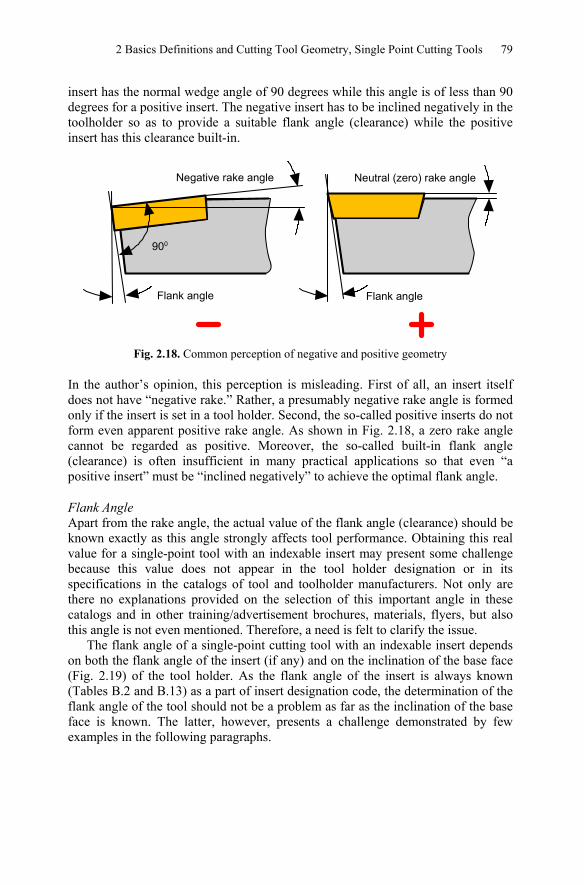
Rake Angle Tools manufacturers made distinction between the so-called negative and positive insert geometry as shown in Fig. 2.18. According to this perception, a negative
2 Basics Definitions and Cutting Tool Geometry, Single Point Cutting Tools 79
insert has the normal wedge angle of 90 degrees while this angle is of less than 90 degrees for a positive insert. The negative insert has to be inclined negatively in the toolholder so as to provide a suitable flank angle (clearance) while the positive insert has this clearance built-in.
Neutral (zero) rake angle
Flank angleFlank angle
Negative rake angle
900
Fig. 2.18. Common perception of negative and positive geometry
In the author’s opinion, this perception is misleading. First of all, an insert itself does not have “negative rake.” Rather, a presumably negative rake angle is formed only if the insert is set in a tool holder. Second, the so-called positive inserts do not form even apparent positive rake angle. As shown in Fig. 2.18, a zero rake angle cannot be regarded as positive. Moreover, the so-called built-in flank angle (clearance) is often insufficient in many practical applications so that even “a positive insert” must be “inclined negatively” to achieve the optimal flank angle.
Flank Angle Apart from the rake angle, the actual value of the flank angle (clearance) should be known exactly as this angle strongly affects tool performance. Obtaining this real value for a single-point tool with an indexable insert may present some challenge because this value does not appear in the tool holder designation or in its specifications in the catalogs of tool and toolholder manufacturers. Not only are there no explanations provided on the selection of this important angle in these catalogs and in other training/advertisement brochures, materials, flyers, but also this angle is not even mentioned. Therefore, a need is felt to clarify the issue.
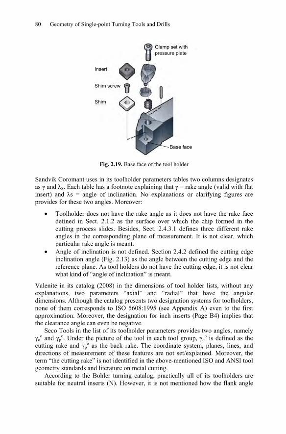
The flank angle of a single-point cutting tool with an indexable insert depends on both the flank angle of the insert (if any) and on the inclination of the base face (Fig. 2.19) of the tool holder. As the flank angle of the insert is always known (Tables B.2 and B.13) as a part of insert designation code, the determination of the flank angle of the tool should not be a problem as far as the inclination of the base face is known. The latter, however, presents a challenge demonstrated by few examples in the following paragraphs.
80 Geometry of Single-point Turning Tools and Drills
Base face
Clamp set withpressure plate
Insert
Shim screw
Shim
Fig. 2.19. Base face of the tool holder
Sandvik Coromant uses in its toolholder parameters tables two columns designates as γ and λS. Each table has a footnote explaining that γ = rake angle (valid with flat insert) and λs = angle of inclination. No explanations or clarifying figures are provides for these two angles. Moreover:
• Toolholder does not have the rake angle as it does not have the rake face defined in Sect. 2.1.2 as the surface over which the chip formed in the cutting process slides. Besides, Sect. 2.4.3.1 defines three different rake angles in the corresponding plane of measurement. It is not clear, which particular rake angle is meant.
• Angle of inclination is not defined. Section 2.4.2 defined the cutting edge inclination angle (Fig. 2.13) as the angle between the cutting edge and the reference plane. As tool holders do not have the cutting edge, it is not clear what kind of “angle of inclination” is meant.
Valenite in its catalog (2008) in the dimensions of tool holder lists, without any explanations, two parameters “axial” and “radial” that have the angular dimensions. Although the catalog presents two designation systems for toolholders, none of them corresponds to ISO 5608:1995 (see Appendix A) even to the first approximation. Moreover, the designation for inch inserts (Page B4) implies that the clearance angle can even be negative.
Seco Tools in the list of its toolholder parameters provides two angles, namely γo
o and γpo. Under the picture of the tool in each tool group, γo
o is defined as the cutting rake and γp
o as the back rake. The coordinate system, planes, lines, and directions of measurement of these features are not set/explained. Moreover, the term “the cutting rake” is not identified in the above-mentioned ISO and ANSI tool geometry standards and literature on metal cutting.
According to the Bohler turning catalog, practically all of its toolholders are suitable for neutral inserts (N). However, it is not mentioned how the flank angle
2 Basics Definitions and Cutting Tool Geometry, Single Point Cutting Tools 81
(relief) is provided by these tool holders. The same can be said about the Ingersoll turning tool catalog.
Kennametal combines Sandvik Coromant and Seco designations, namely, for some toolholders λS° γO° and for others γF° γP° are listed in its catalog. The mentioned angles are not clearly defined or explained.
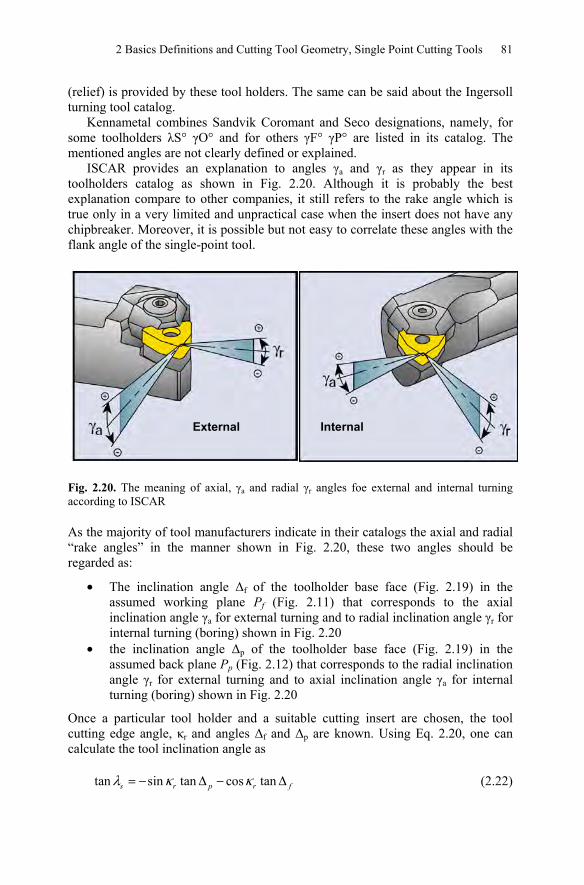
ISCAR provides an explanation to angles γa and γr as they appear in its toolholders catalog as shown in Fig. 2.20. Although it is probably the best explanation compare to other companies, it still refers to the rake angle which is true only in a very limited and unpractical case when the insert does not have any chipbreaker. Moreover, it is possible but not easy to correlate these angles with the flank angle of the single-point tool.
Fig. 2.20. The meaning of axial, γa and radial γr angles foe external and internal turning according to ISCAR
As the majority of tool manufacturers indicate in their catalogs the axial and radial “rake angles” in the manner shown in Fig. 2.20, these two angles should be regarded as:
• The inclination angle Δf of the toolholder base face (Fig. 2.19) in the assumed working plane Pf (Fig. 2.11) that corresponds to the axial inclination angle γa for external turning and to radial inclination angle γr for internal turning (boring) shown in Fig. 2.20
• the inclination angle Δp of the toolholder base face (Fig. 2.19) in the assumed back plane Pp (Fig. 2.12) that corresponds to the radial inclination angle γr for external turning and to axial inclination angle γa for internal turning (boring) shown in Fig. 2.20
Once a particular tool holder and a suitable cutting insert are chosen, the tool cutting edge angle, κr and angles Δf and Δp are known. Using Eq. 2.20, one can calculate the tool inclination angle as
tan sin tan cos tans r p r fλ κ κ= − Δ − Δ (2.22)
External Internal
82 Geometry of Single-point Turning Tools and Drills
Using this calculated value, one can combine Eqs. 2.14 and 2.18 to calculate the normal flank angle as
( )1arctan
cos cos cot sin cotns r p r f
αλ κ κ
=− Δ − Δ
(2.23)
Note that if the selected insert is not neutral (N) but rather has a flank angle, this angle should be added to that calculated using Eq. 2.24.
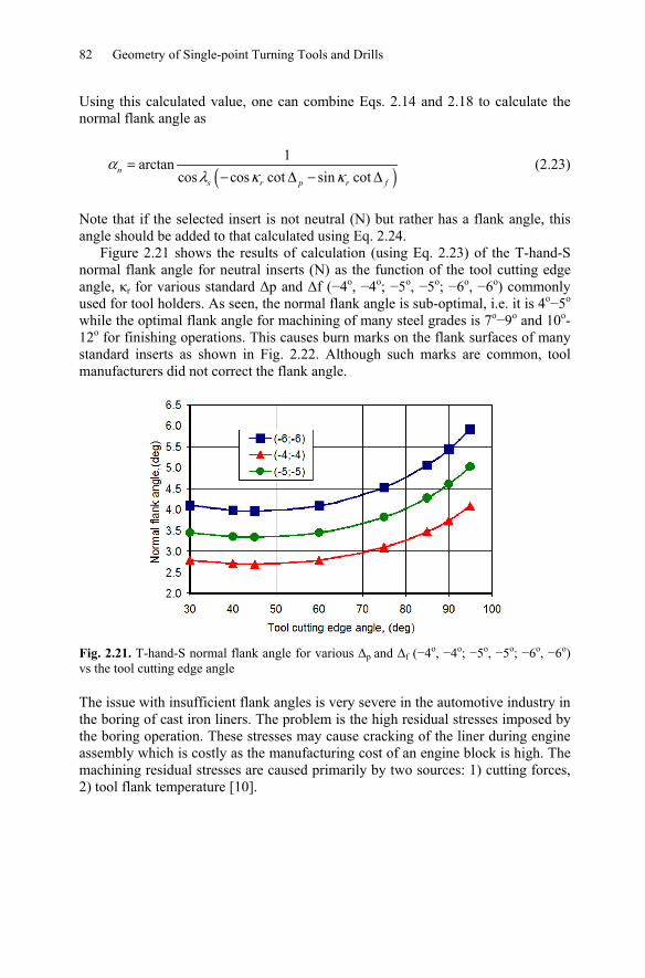
Figure 2.21 shows the results of calculation (using Eq. 2.23) of the T-hand-S normal flank angle for neutral inserts (N) as the function of the tool cutting edge angle, κr for various standard Δp and Δf (−4o, −4o; −5o, −5o; −6o, −6o) commonly used for tool holders. As seen, the normal flank angle is sub-optimal, i.e. it is 4o−5o while the optimal flank angle for machining of many steel grades is 7o−9o and 10o-12o for finishing operations. This causes burn marks on the flank surfaces of many standard inserts as shown in Fig. 2.22. Although such marks are common, tool manufacturers did not correct the flank angle.
Fig. 2.21. T-hand-S normal flank angle for various Δp and Δf (−4o, −4o; −5o, −5o; −6o, −6o) vs the tool cutting edge angle
The issue with insufficient flank angles is very severe in the automotive industry in the boring of cast iron liners. The problem is the high residual stresses imposed by the boring operation. These stresses may cause cracking of the liner during engine assembly which is costly as the manufacturing cost of an engine block is high. The machining residual stresses are caused primarily by two sources: 1) cutting forces, 2) tool flank temperature [10].
2 Basics Definitions and Cutting Tool Geometry, Single Point Cutting Tools 83
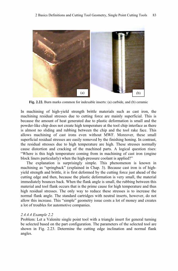
Fig. 2.22. Burn marks common for indexable inserts: (a) carbide, and (b) ceramic
In machining of high-yield strength brittle materials such as cast iron, the machining residual stresses due to cutting force are mainly superficial. This is because the amount of heat generated due to plastic deformation is small and the powder-like chip does not create high temperature at the tool chip interface as there is almost no sliding and rubbing between the chip and the tool rake face. This allows machining of cast irons even without MWF. Moreover, these small superficial residual stresses are easily removed by the finishing honing. In contrast, the residual stresses due to high temperature are high. These stresses normally cause distortion and cracking of the machined parts. A logical question rises: “Where is this high temperature coming from in machining of cast iron (engine block liners particularly) when the high-pressure coolant is applied?”
The explanation is surprisingly simple. This phenomenon is known in machining as “springback” (explained in Chap. 3). Because cast iron is of high-yield strength and brittle, it is first deformed by the cutting force just ahead of the cutting edge and then, because the plastic deformation is very small, the material immediately bounces back. When the flank angle is small, the rubbing between this material and tool flank occurs that is the prime cause for high temperature and thus high residual stresses. The only way to reduce these stresses is to increase the normal flank angle. The standard cartridges with neutral inserts, however, do not allow this increase. This “simple” geometry issue costs a lot of money and creates a lot of troubles for automotive companies.
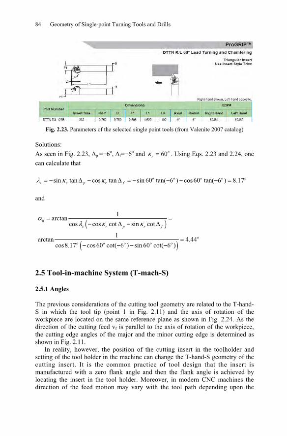
2.4.4.4 Example 2.2 Problem: Let a Valenite single point tool with a triangle insert for general turning be selected based on the part configuration. The parameters of the selected tool are shown in Fig. 2.23. Determine the cutting edge inclination and normal flank angles.
(a) (b)
84 Geometry of Single-point Turning Tools and Drills
Fig. 2.23. Parameters of the selected single point tools (from Valenite 2007 catalog)
Solutions: As seen in Fig. 2.23, Δp =−6o, Δf=−6o and 60o
rκ = . Using Eqs. 2.23 and 2.24, one can calculate that
sin tan cos tan sin 60 tan( 6 ) cos 60 tan( 6 ) 8.17o o o o os r p r fλ κ κ= − Δ − Δ = − − − − =
and
( )
( )
1arctancos cos cot sin cot
1arctan 4.44cos8.17 cos 60 cot( 6 ) sin 60 cot( 6 )
ns r p r f
oo o o o o
αλ κ κ
= =− Δ − Δ
=− − − −
2.5 Tool-in-machine System (T-mach-S)
2.5.1 Angles
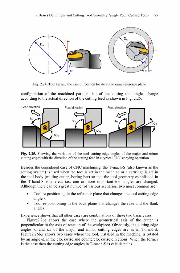
The previous considerations of the cutting tool geometry are related to the T-hand-S in which the tool tip (point 1 in Fig. 2.11) and the axis of rotation of the workpiece are located on the same reference plane as shown in Fig. 2.24. As the direction of the cutting feed vf is parallel to the axis of rotation of the workpiece, the cutting edge angles of the major and the minor cutting edge is determined as shown in Fig. 2.11.
In reality, however, the position of the cutting insert in the toolholder and setting of the tool holder in the machine can change the T-hand-S geometry of the cutting insert. It is the common practice of tool design that the insert is manufactured with a zero flank angle and then the flank angle is achieved by locating the insert in the tool holder. Moreover, in modern CNC machines the direction of the feed motion may vary with the tool path depending upon the
2 Basics Definitions and Cutting Tool Geometry, Single Point Cutting Tools 85
Fig. 2.24. Tool tip and the axis of rotation locate at the same reference plane
configuration of the machined part so that of the cutting tool angles change according to the actual direction of the cutting feed as shown in Fig. 2.25.
Fig. 2.25. Showing the variation of the tool cutting edge angles of the major and minor cutting edges with the direction of the cutting feed in a typical CNC copying operation
Besides the considered case of CNC machining, the T-mach-S (also known as the setting system) is used when the tool is set in the machine or a cartridge is set in the tool body (milling cutter, boring bar) so that the tool geometry established in the T-hand-S is altered, i.e., one or more important tool angles are changed. Although there can be a great number of various scenarios, two most common are:
• Tool re-positioning in the reference plane that changes the tool cutting edge angle κr
• Tool re-positioning in the back plane that changes the rake and the flank angles
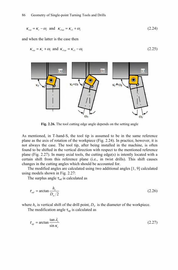
Experience shows that all other cases are combinations of these two basic cases. Figure2.26a shows the case where the geometrical axis of the cutter is
perpendicular to the axis of rotation of the workpiece. Obviously, the cutting edge angles κr and κr1 of the major and minor cutting edges are as in T-hand-S. Figure2.26b,c shows two cases where the tool, installed in the machine, is rotated by an angle ωr in the clockwise and counterclockwise directions. When the former is the case then the cutting edge angles in T-mach-S is calculated as
86 Geometry of Single-point Turning Tools and Drills
r r rωκ κ ω= − and 1 1r r rωκ κ ω= + (2.24)
and when the latter is the case then
1r rωκ κ ω= + and 1 1 1r rωκ κ ω= − (2.25)
Fig. 2.26. The tool cutting edge angle depends on the setting angle
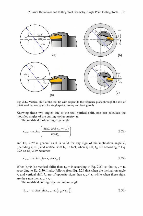
As mentioned, in T-hand-S, the tool tip is assumed to be in the same reference plane as the axis of rotation of the workpiece (Fig. 2.24). In practice, however, it is not always the case. The tool tip, after being installed in the machine, is often found to be shifted in the vertical direction with respect to the mentioned reference plane (Fig. 2.27). In many axial tools, the cutting edge(s) is intently located with a certain shift from this reference plane (i.e., in twist drills). This shift causes changes in the cutting angles which should be accounted for.
The modified angles are calculated using two additional angles [1, 9] calculated using models shown in Fig. 2.27:
The surplus angle τad is calculated as
arctan2
oad
w
hD
τ = (2.26)
where ho is vertical shift of the drill point, Dw is the diameter of the workpiece. The modification angle τap is calculated as
tanarctan
sins
apr
λτκ
= (2.27)
2 Basics Definitions and Cutting Tool Geometry, Single Point Cutting Tools 87
Fig. 2.27. Vertical shift of the tool tip with respect to the reference plane through the axis of rotation of the workpiece for single-point turning and boring tools
Knowing these two angles due to the tool vertical shift, one can calculate the modified angles of the cutting tool geometry as:
The modified tool cutting edge angle
( )tan cosarctan
cosr ap ad
r map
κ τ τκ
τ−
⎛ ⎞−⎜ ⎟=⎜ ⎟⎝ ⎠
(2.28)
and Eq. 2.29 is general as it is valid for any sign of the inclination angle λs (including λs = 0) and vertical shift ho. In fact, when λs = 0, τap = 0 according to Eq. 2.28 so Eq. 2.29 becomes
( )arctan tan cosr m r adκ κ τ− = (2.29)
When h0=0 (no vertical shift) then τad = 0 according to Eq. 2.27, so that κr-m = κr according to Eq. 2.30. It also follows from Eq. 2.29 that when the inclination angle λs and vertical shift ho are of opposite signs then κr-m< κr while when these signs are the same then κr-m> κr .
The modified cutting edge inclination angle
( )( )arctan sin tans m r m ap adλ κ τ τ− −= − (2.30)
(a) (b)
(c) (d)
88 Geometry of Single-point Turning Tools and Drills
Equation 2.31 is valid for any sign of the inclination angle λs (including λs = 0) and vertical shift ho.
The modified orthogonal rake angle
( )tanarctan tan tan
cosp ad
o m r m s mr m
γ τγ κ λ
κ− − −−
⎛ ⎞+⎜ ⎟= +⎜ ⎟⎝ ⎠
(2.31)
where the back rake angle γp calculates using Eq. 2.7. Equation 2.32 is valid for any sign of the inclination angle λs (including λs = 0) and vertical shift ho. When h0
= 0 (no vertical shift) then τad = 0 according to Eq. 2.27, κr-m = κr and λsm = λs so that γo-m = γoaccording to Eq. 2.18.
The modified orthogonal flank angle
( )( )arctan tan coso m p ad r mα α τ κ− −= − (2.32)
where the back rake angle αp calculates using Eq. 2.19. Equation 2.33 is valid for any sign of the inclination angle λs (including λs = 0) and vertical shift ho. When h0
= 0 (no vertical shift) then τad = 0 according to Eq. 2.27, κr-m= κr and λsm = λs so that αo-m= αo according to Eq. 2.19.
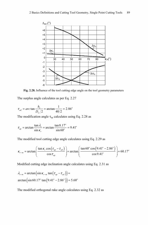
Figure 2.28 shows deviations Δan of the tool cutting edge angle, Δκr, orthogonal rake angle, Δγo, orthogonal flank angle, Δαo, and cutting edge inclination angle, Δλs as functions of the tool cutting edge angle when a single point cutting tool having normal rake angle, γn = 10o, normal flank angle, αn = 8o, and cutting edge inclination angle, λs = 10o, is installed with h0 = 2mm (Fig. 2.27a). The diameter of the workpiece Dw=30mm.
As seen in Fig. 2.28, the cutting tool inclination angle changes significantly while deviations of the orthogonal rake and flank angles diminish in the region of the widely used tool cutting edge angle. However, the deviation of the flank angle cannot be ignored for tools with neutral (N) indexable inserts.
2.5.2 Example 2.3
Problem: Let the cutting tool discussed in Example 2 be elevated by h0=1mm with respect to the reference plane containing the axis of rotation of the workpiece (Fig. 2.27) in machining of a workpiece having diameter Dw=40mm. Determine the geometry of this tool in the tool-in-machine system. Solution: The tool selected in Example 2 has the following geometrical parameters: normal flank angle αn=44.4o, cutting edge inclination angle λs=8.17o, tool cutting edge angle κr=60o, back rake angle γp=−6o.
2 Basics Definitions and Cutting Tool Geometry, Single Point Cutting Tools 89
+6
+5
+4
+3
+2
+1
0
-1
-2
-3
-4
-5
-6
30 40 50 60 70 80
o
r
rrr
,(°)
(°)
an
ΔγΔκ
κ
oΔα
sΔλ
Fig. 2.28. Influence of the tool cutting edge angle on the tool geometry parameters
The surplus angle calculates as per Eq. 2.27
1tan arctan 2.862 40 2
ooad
w
harc
Dτ = = =
The modification angle τap calculates using Eq. 2.28 as
tan tan8.17arctan arctan 9.41sin sin 60
oos
ap or
λτκ
= = =
The modified tool cutting edge angle calculates using Eq. 2.29 as
( ) ( )tan 60 cos 9.41 2.86tan cosarctan arctan 60.17
cos cos9.41
o o or ap ad o
r m oap
κ τ τκ
τ−
⎛ ⎞⎛ ⎞ −−⎜ ⎟⎜ ⎟= = =
⎜ ⎟ ⎜ ⎟⎝ ⎠ ⎝ ⎠ Modified cutting edge inclination angle calculates using Eq. 2.31 as
( )( )( )( )
arctan sin tan
arctan sin 60.17 tan 9.41 2.86 5.68
s m r m ap ad
o o o o
λ κ τ τ− −= − =
− =
The modified orthogonal rake angle calculates using Eq. 2.32 as
90 Geometry of Single-point Turning Tools and Drills
( )
( )( )
tanarctan tan tan
cos
tan 6 2.86arctan tan 60.17 tan 5.68 2.20
cos 60.17
p ado m r m s m
r m
o oo o o
o
γ τγ κ λ
κ− − −−
⎛ ⎞+⎜ ⎟= + =⎜ ⎟⎝ ⎠
⎛ ⎞− +⎜ ⎟+ = −⎜ ⎟⎝ ⎠
The modified normal rake angle calculates using Eq. 2.16 as
( ) ( )( )arctan tan cos arctan tan 2.20 cos5.68 2.19o o on m o m s mγ γ λ− − −= = − = −
The back flank angle calculates using Eq. 2.12 as
tan tan 4.44arctan arctan 8.83cos cos60
oon
p or
αακ
⎛ ⎞ ⎛ ⎞= = =⎜ ⎟ ⎜ ⎟
⎝ ⎠ ⎝ ⎠
The modified orthogonal flank angle calculates using Eq. 2.33 as
( )( )( )( )
arctan tan cos
arctan tan 8.83 2.85 cos60.17 2.98
o m p ad r m
o
α α τ κ− −= − =
− =
And finally, the modified normal flank angle calculates using Eq. 2.14 as
tan tan 3.07arctan arctan 3.08cos cos5.68
ooo m
n m os m
ααλ
−−
−
⎛ ⎞ ⎛ ⎞= = =⎜ ⎟ ⎜ ⎟
⎝ ⎠⎝ ⎠
2.6 Tool-in-use System (T-use-S)
The T-use-S considers the geometry of the cutting tool accounting for machining kinematics. When the cutting tool is being used, the actual direction of the primary motion and the feed motion may differ from the assumed directions in the T-hand-S and T-mach-S. Moreover, the actual tool path may be different compare to that assumed in the T-hand-S and T-mach-S due to several feed motions applied simultaneously as multi-axis machines are widely used. As the parameters of the tool geometry are affected by the actual resultant motion of the cutting tool relative to the workpiece, a new system, referred to as the tool-in-use system (T-use-S) coordinate system should be considered and the corresponding tool angles, referred to as the working angles, should be established in this new system.
2 Basics Definitions and Cutting Tool Geometry, Single Point Cutting Tools 91
Although such a system has been known for years, its importance is growing due to the following facts:
• Demand for increasing productivity of machining has been resulting in the development of stronger tool materials with advanced coatings that allow higher feed rates. Today, these rates, particularly in machining aluminum alloys in the aerospace and automotive industries, are so great that they can significantly affect the direction of the resultant cutting motion.
• Wide use of multi-axis machines results in the utilization of multi-feed cutting to produce the so-called sculptured surfaces. These feeds also change the direction of the resultant motion that affects the cutting tool geometry.
• Wide use of CNC machines and production lines gave rise to so-called contour machining where the same tool is used to machine the complete contour or profile of a part as shown in Fig. 2.25. As such, the tool geometry parameters vary depending upon a particular segment of the contour because the tool cutting edge angles of the major and minor cutting edges vary as well as the cutting feed.
2.6.1 Reference Planes
The basis of the T-use-S is the tool in use reference plane Pre. Similar to Pr, the position of this reference plane is defined as being perpendicular to the vector of the resultant motion. Once Pre is defined, the following system of planes (similar to that shown in Fig. 2.12) can be defined:
• The T-use-S working plane, Pef is perpendicular to the reference plane Pre and contains the direction of the resultant motion.
• The T-use-S cutting edge plane Pse is perpendicular to Pre, and contains the major cutting edge. Similar to the T-hand-S, if the major cutting edge is a straight line then the tool cutting edge plane is the same for any point of this edge. This plane is fully defined by two intersecting lines, namely, by the straight cutting edge and the vector of the cutting speed. If, however, the major cutting edge is not straight then there are an infinite number of tool cutting edge planes. As such, a tool cutting edge plane should be determined for each point of the curved cutting edge as the plane which tangent to the cutting edge at the point of consideration and which contains the vector of the cutting speed (or perpendicular to the main reference plane).
• The T-use-S back plane Ppe is perpendicular to Pre and Pfe. • Perpendicular to the projection of the cutting edge into the reference plane
is the T-use-S orthogonal plane Poe. When the cutting edge is not straight, there are an infinite number of orthogonal planes defined for each given point of the curved cutting edge, and the orthogonal plane is defined as the plane which is perpendicular to the tangent to the projection of the cutting edge into the reference plane edge at the point of consideration.
92 Geometry of Single-point Turning Tools and Drills
• The T-use-S cutting edge normal plane Pne. According to ISO and ANSI standards [3, 7], this plane is identical to the cutting edge normal plane defined in the T-hand-S, i.e., ne nP P≡ . In the author’s opinion, this notion is incorrect as it is not based on the physics of the metal cutting process. This physics implies that the proper rake and flank angles in the T-use-S are measured in a plane containing the resultant direction of chip flow. As Pne defined by the abovementioned standards does not contain this direction, it lacks physical sense. In the author’s opinion, Pne should be defined as to be perpendicular to the equivalent cutting edge (discussed later).
The angles of the cutting tool in the T-use-S are defined in these planes in the same manner as in the T-hand-S.
2.6.2 The Concept
The foregoing analysis implies that the basis of the T-use-S is the proper determination of the reference plane Pre. To do that, the direction of the resultant motion should be identified. As discussed in Appendix A (Fig. A.7), this direction, defined by the directional vector ve is the vectorial sum of the directional vector of prime motion v and the directional vector of the resultant feed motion vf [9], i.e.,
e f= +v v v (2.33)
This directional vector is always tangential to the trajectory of the resultant tool motion.
As the flank angle (clearance) is to clear a certain motion, the following equation for the T-use-S flank angle can be written on the basis of Eq. 2.34
e vfα α α= ± (2.34)
Depending on particular direction(s) of feed motion(s), the kinematic flank angle due to these motions may increase or decrease the T-hand-S flank angle. This is accounted for by the ± sign in Eq. 2.35.
2.6.3 Modification of the T-hand-S Tool Geometry
Figure 2.29 presents the simplest example of a shaping operation where the prime motion is straight having velocity v. As seen in Fig. 2.29a, a square bar stock is used as a tool. The side face of this bar stock is used as the rake face having cutting edge ab and thus the rake angle γ is zero. The square face of this bar stock abcd is used as the flank face so the flank angle α is also zero. The tool thus formed is set to cut the chip having chip thickness t1.
When the tool moves in the direction of the prime motion (along the z-axis) with velocity v and the chip is formed (Fig. 2.29b), the force (energy) needed for tool penetration into the workpiece consists of three parts: (1) the force (energy)

2 Basics Definitions and Cutting Tool Geometry, Single Point Cutting Tools 93
needed for chip formation, i.e., for separation of the layer being removed (having width dw and height t1) from the rest of the workpiece, (2) the friction force (energy) due to friction at the tool-chip interface over the rake face and (3) the friction force (energy) due to friction of the flank face abcd and the machined surface. Note that such machining is possible only theoretically where it can be assumed for the sake of discussion that no elastic recovery (springback) of the work material occurs (the work material is perfectly plastic).
Fig. 2.29. Formation of the tool from a square bar stock in planing
Out of these three forces (energies), the first and second are unavoidable as it represents the essence of the cutting process. In contrast, the friction force on the tool flank abcd must be significantly reduced for the very existence of the process. To do that, the flank surface should always be made with a certain flank angle (relief) α > 0o as shown in Fig. 2.29c. The square bar stock having α > 0o thus becomes the cutting tool.
The above example implies that the major distinguishing feature of the cutting tool is the flank face having a flank angle α > 0o. The rake angle can be positive,
94 Geometry of Single-point Turning Tools and Drills
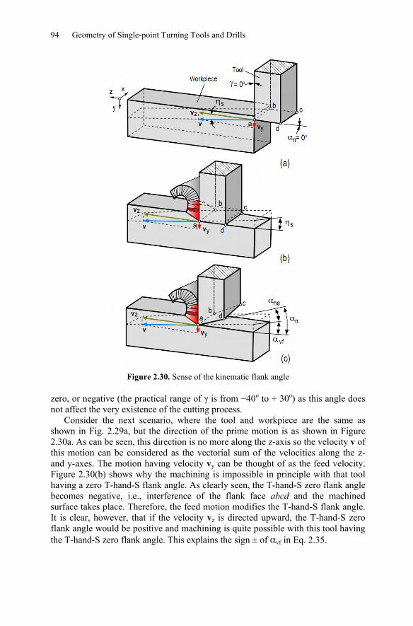
Figure 2.30. Sense of the kinematic flank angle
zero, or negative (the practical range of γ is from −40o to + 30o) as this angle does not affect the very existence of the cutting process.
Consider the next scenario, where the tool and workpiece are the same as shown in Fig. 2.29a, but the direction of the prime motion is as shown in Figure 2.30a. As can be seen, this direction is no more along the z-axis so the velocity v of this motion can be considered as the vectorial sum of the velocities along the z- and y-axes. The motion having velocity vy can be thought of as the feed velocity. Figure 2.30(b) shows why the machining is impossible in principle with that tool having a zero T-hand-S flank angle. As clearly seen, the T-hand-S zero flank angle becomes negative, i.e., interference of the flank face abcd and the machined surface takes place. Therefore, the feed motion modifies the T-hand-S flank angle. It is clear, however, that if the velocity vz is directed upward, the T-hand-S zero flank angle would be positive and machining is quite possible with this tool having the T-hand-S zero flank angle. This explains the sign ± of αvf in Eq. 2.35.
2 Basics Definitions and Cutting Tool Geometry, Single Point Cutting Tools 95
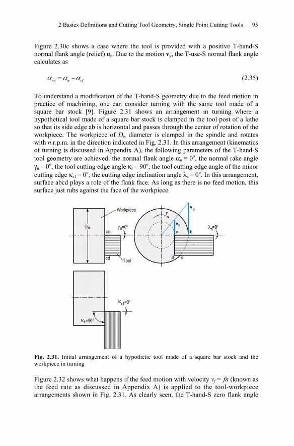
Figure 2.30c shows a case where the tool is provided with a positive T-hand-S normal flank angle (relief) αn. Due to the motion vy, the T-use-S normal flank angle calculates as
ne n vfα α α= − (2.35)
To understand a modification of the T-hand-S geometry due to the feed motion in practice of machining, one can consider turning with the same tool made of a square bar stock [9]. Figure 2.31 shows an arrangement in turning where a hypothetical tool made of a square bar stock is clamped in the tool post of a lathe so that its side edge ab is horizontal and passes through the center of rotation of the workpiece. The workpiece of Dw diameter is clamped in the spindle and rotates with n r.p.m. in the direction indicated in Fig. 2.31. In this arrangement (kinematics of turning is discussed in Appendix A), the following parameters of the T-hand-S tool geometry are achieved: the normal flank angle αn = 0o, the normal rake angle γn = 0o, the tool cutting edge angle κr = 90o, the tool cutting edge angle of the minor cutting edge κr1 = 0o, the cutting edge inclination angle λs = 0o. In this arrangement, surface abcd plays a role of the flank face. As long as there is no feed motion, this surface just rubs against the face of the workpiece.
Fig. 2.31. Initial arrangement of a hypothetic tool made of a square bar stock and the workpiece in turning
Figure 2.32 shows what happens if the feed motion with velocity vf = fn (known as the feed rate as discussed in Appendix A) is applied to the tool-workpiece arrangements shown in Fig. 2.31. As clearly seen, the T-hand-S zero flank angle
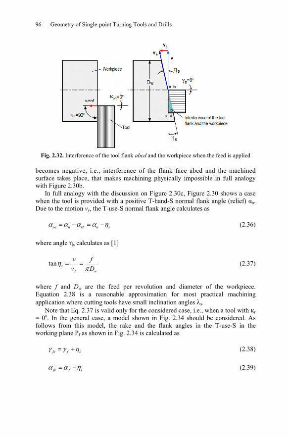
96 Geometry of Single-point Turning Tools and Drills
Fig. 2.32. Interference of the tool flank abcd and the workpiece when the feed is applied
becomes negative, i.e., interference of the flank face abcd and the machined surface takes place, that makes machining physically impossible in full analogy with Figure 2.30b.
In full analogy with the discussion on Figure 2.30c, Figure 2.30 shows a case when the tool is provided with a positive T-hand-S normal flank angle (relief) αn. Due to the motion vy, the T-use-S normal flank angle calculates as
ne n vf n sα α α α η= − = − (2.36)
where angle ηs calculates as [1]
tan sf w
v fv D
ηπ
= = (2.37)
where f and Dw are the feed per revolution and diameter of the workpiece. Equation 2.38 is a reasonable approximation for most practical machining application where cutting tools have small inclination angles λs.
Note that Eq. 2.37 is valid only for the considered case, i.e., when a tool with κr = 0o. In the general case, a model shown in Fig. 2.34 should be considered. As follows from this model, the rake and the flank angles in the T-use-S in the working plane Pf as shown in Fig. 2.34 is calculated as
fe f sγ γ η= + (2.38)
fe f sα α η= − (2.39)
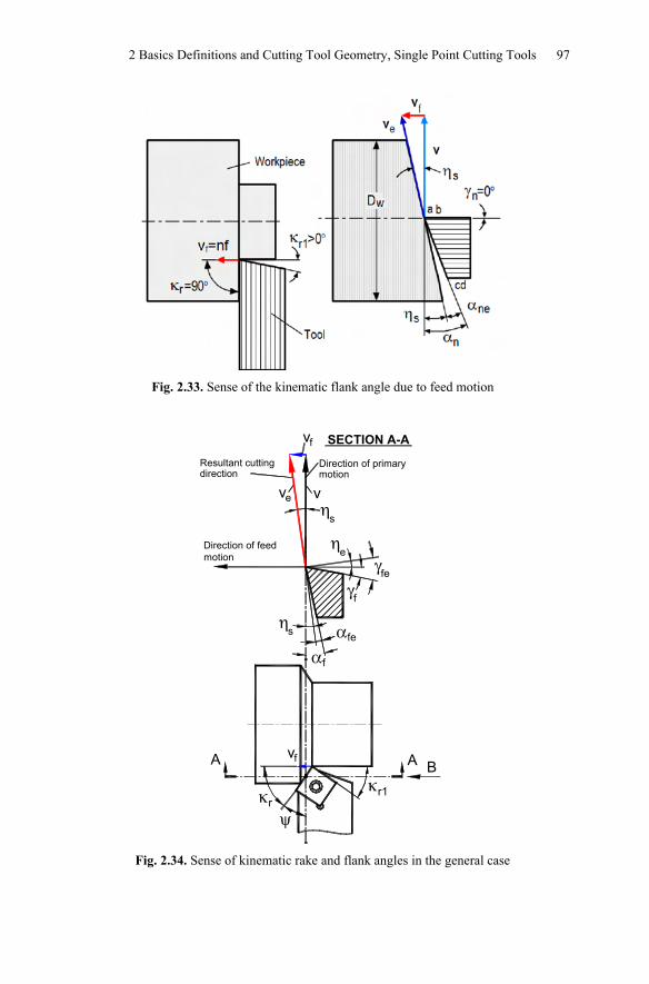
2 Basics Definitions and Cutting Tool Geometry, Single Point Cutting Tools 97
Fig. 2.33. Sense of the kinematic flank angle due to feed motion
vf
ve
Direction of primarymotion
Resultant cuttingdirection
SECTION A-A
η
γ
α
κκ
ψ
A A B
s
v
Direction of feedmotion
fe
fe
vf
rr1
γf
ηe
αf
ηs
Fig. 2.34. Sense of kinematic rake and flank angles in the general case
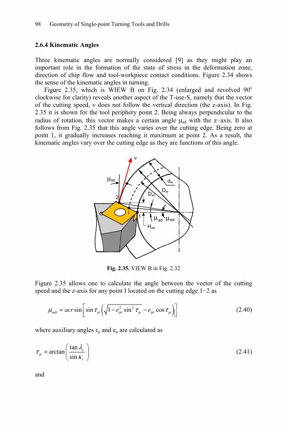
98 Geometry of Single-point Turning Tools and Drills
2.6.4 Kinematic Angles
Three kinematic angles are normally considered [9] as they might play an important role in the formation of the state of stress in the deformation zone, direction of chip flow and tool-workpiece contact conditions. Figure 2.34 shows the sense of the kinematic angles in turning.
Figure 2.35, which is WIEW B on Fig. 2.34 (enlarged and revolved 90o clockwise for clarity) reveals another aspect of the T-use-S, namely that the vector of the cutting speed, v does not follow the vertical direction (the z-axis). In Fig. 2.35 it is shown for the tool periphery point 2. Being always perpendicular to the radius of rotation, this vector makes a certain angle μad with the z−axis. It also follows from Fig. 2.35 that this angle varies over the cutting edge. Being zero at point 1, it gradually increases reaching it maximum at point 2. As a result, the kinematic angles vary over the cutting edge as they are functions of this angle.
Dw
μad
Had
dw
Dw
2
1i
Dwi
μadi
μad
v
Fig. 2.35. VIEW B in Fig. 2.32
Figure 2.35 allows one to calculate the angle between the vector of the cutting speed and the z-axis for any point I located on the cutting edge 1−2 as
( )2 2sin sin 1 sin cosadi i iacr e eμ μ μ μ μμ τ τ τ⎡ ⎤= − −⎢ ⎥⎣ ⎦ (2.40)
where auxiliary angles τμ and eμ are calculated as
tanarctan
sins
rμ
λτκ
⎛ ⎞= ⎜ ⎟
⎝ ⎠ (2.41)
and
2 Basics Definitions and Cutting Tool Geometry, Single Point Cutting Tools 99
21 w
iwi
de
Dμ = − (2.42)
The cutting edge inclination angle λsei is the angle between the cutting edge and the plane perpendicular to the resultant cutting direction. It is calculated as [1]
cos cos sin sin cos sin cossin cos cos
sei r s si r s adi si
s si adi
λ κ λ η κ λ μ ηλ η μ= + +
(2.43)
where
arctan arctanfsi
i wi
v fv D
ηπ
⎛ ⎞ ⎛ ⎞= =⎜ ⎟ ⎜ ⎟
⎝ ⎠ ⎝ ⎠ (2.44)
In practice, however, this angle is calculated for periphery point 2 (Fig. 2.35). In this case, Eq. 2.41 becomes
2 sinarctan
sin cosw s
adw r s
dD
λμκ λ
⎛ ⎞= ⎜ ⎟
⎝ ⎠ (2.45)
In practice, the inclination angle λs is small for general turning tools so the variation of λse over the cutting edge can be safely neglected. This is not the case, however, with many other tools such as drills, milling tools, hobs, etc., where this variation must be considered in an analysis of cutting tool geometry and its influence on the cutting process.
In a particular case when λs = 0, as it follows from Eq. 2.46, μad then it follows from Eq. 2.44 that
cos sinse r sλ κ η= (2.46)
Kinematic rake angle calculates as
2 2
tansin arctan sin
cosarcsin 1 sin cos
tancos arctan cos sin
cos
sin cos cos sin
sr si
nei n sei
sr si adi
n
n s si adi
λκ ηγ
γ γ λλκ η μγ
γ λ η μ
⎡ ⎤⎛ ⎞⎛ ⎞+ +⎢ ⎥⎜ ⎟⎜ ⎟⎜ ⎟⎢ ⎥⎝ ⎠⎝ ⎠= − +⎢ ⎥
⎛ ⎞⎛ ⎞⎢ ⎥+⎜ ⎟⎜ ⎟⎢ ⎥⎜ ⎟⎝ ⎠⎝ ⎠⎣ ⎦
(2.47)
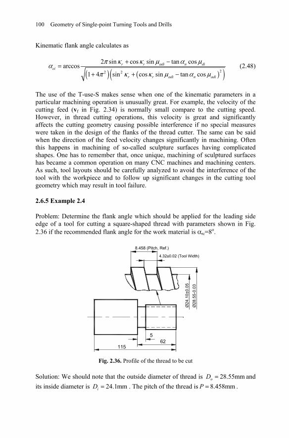
100 Geometry of Single-point Turning Tools and Drills
Kinematic flank angle calculates as
( ) ( )( )22 2
2 sin cos sin tan cosarccos
1 4 sin cos sin tan cos
r r adi n diei
r r adi n adi
π κ κ μ α μαπ κ κ μ α μ
+ −=
+ + − (2.48)
The use of the T-use-S makes sense when one of the kinematic parameters in a particular machining operation is unusually great. For example, the velocity of the cutting feed (vf in Fig. 2.34) is normally small compare to the cutting speed. However, in thread cutting operations, this velocity is great and significantly affects the cutting geometry causing possible interference if no special measures were taken in the design of the flanks of the thread cutter. The same can be said when the direction of the feed velocity changes significantly in machining. Often this happens in machining of so-called sculpture surfaces having complicated shapes. One has to remember that, once unique, machining of sculptured surfaces has became a common operation on many CNC machines and machining centers. As such, tool layouts should be carefully analyzed to avoid the interference of the tool with the workpiece and to follow up significant changes in the cutting tool geometry which may result in tool failure.
2.6.5 Example 2.4
Problem: Determine the flank angle which should be applied for the leading side edge of a tool for cutting a square-shaped thread with parameters shown in Fig. 2.36 if the recommended flank angle for the work material is αrc=8o.
4.32±0.02 (Tool Width)
8.458 (Pitch, Ref.)
Ø24
.10±
0.05
Ø28
.55-
0.03
115
562
Fig. 2.36. Profile of the thread to be cut
Solution: We should note that the outside diameter of thread is 28.55mmoD = and its inside diameter is 24.1mmiD = . The pitch of the thread is 8.458mmP = .
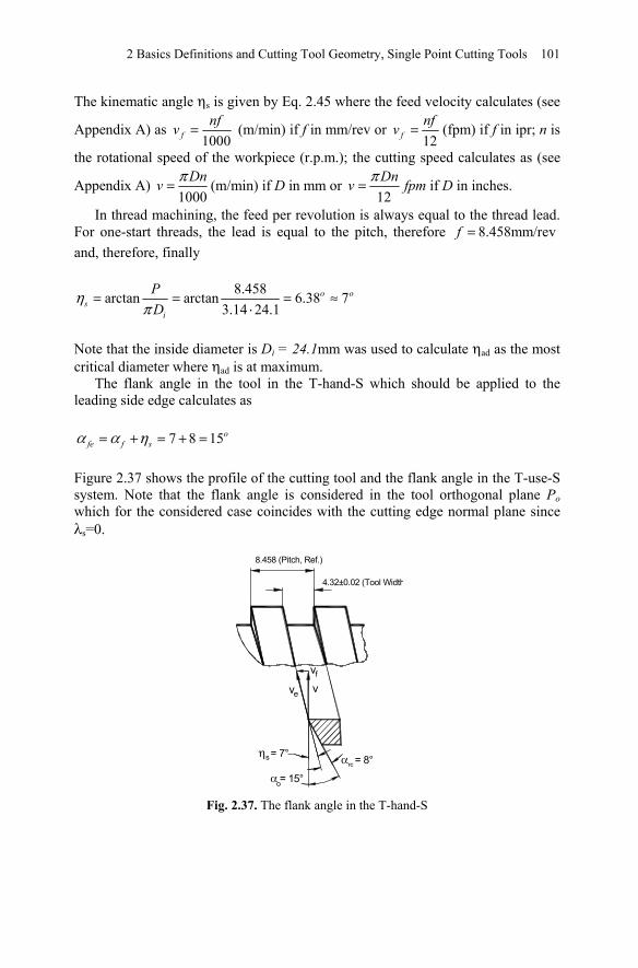
2 Basics Definitions and Cutting Tool Geometry, Single Point Cutting Tools 101
The kinematic angle ηs is given by Eq. 2.45 where the feed velocity calculates (see
Appendix A) as 1000f
nfv = (m/min) if f in mm/rev or 12fnfv = (fpm) if f in ipr; n is
the rotational speed of the workpiece (r.p.m.); the cutting speed calculates as (see
Appendix A) 1000
Dnv π= (m/min) if D in mm or 12Dnv fpmπ= if D in inches.
In thread machining, the feed per revolution is always equal to the thread lead. For one-start threads, the lead is equal to the pitch, therefore 8.458mm/revf = and, therefore, finally
8.458arctan arctan 6.38 73.14 24.1
o os
i
PD
ηπ
= = = ≈⋅
Note that the inside diameter is Di = 24.1mm was used to calculate ηad as the most critical diameter where ηad is at maximum.
The flank angle in the tool in the T-hand-S which should be applied to the leading side edge calculates as
7 8 15ofe f sα α η= + = + =
Figure 2.37 shows the profile of the cutting tool and the flank angle in the T-use-S system. Note that the flank angle is considered in the tool orthogonal plane Po which for the considered case coincides with the cutting edge normal plane since λs=0.
4.32±0.02 (Tool Width
8.458 (Pitch, Ref.)
vve
vf
η = 7°
α = 15°o
rcα = 8°s
Fig. 2.37. The flank angle in the T-hand-S

http://www.springer.com/978-1-84996-052-6