Embed Size (px)
Citation preview

Practical Flow Cytometry in Haematology Diagnosis, First Edition. Mike Leach, Mark Drummond and Allyson Doig.
© 2013 John Wiley & Sons, Ltd. Published 2013 by John Wiley & Sons, Ltd.
3
Principles of Flow Cytometry
Introduction
Over the years, flow cytometry technology, with its
multiple applications, has had a significant impact on
our understanding of cell biology, immunology and
haemopoietic ontogeny, allowing its application to the
diagnostic challenges of clinical medicine.
The basic principle of flow cytometry is inherent in the
ability to analyse multiple characteristics of a single cell
within a heterogenous population, in a short period of
time [1, 2]. The term heterogenous is very important. In
many clinical scenarios it might be far from clear whether
a cellular proliferation is reactive or, indeed, neoplastic.
Furthermore, these populations do not exist in isolation
but within a milieu of other cell types. The diversity of
diseases afflicting the cells of the body compartments
is vast. Clinico-pathological correlation is at the very core
of accurate diagnosis. Ignore the characteristics of either,
at your peril.
Modern flow cytometers have the capability to analyse
several thousands of cells per second. Cells in suspension
pass through a beam of light (usually a laser beam) in
single file; signals generated are related to the size of the
cell and the internal complexity or granularity of the cell,
enabling the cytometer to identify different cell popula-
tions depending on these characteristics. There are a wide
range of applications for flow cytometry in a number
of different disciplines. However, in haematology it
has become an important tool in the identification of
haematological disorders from a wide range of diagnostic
samples, such as peripheral blood, bone marrow, CSF,
pleural effusion, ascitic fluid and lymph node aspirates [1].
For the analysis of solid tissue a cell suspension must first
be made.
There are many books and articles available outlining
the principles of flow cytometry in great detail [1–7].
This chapter is written with the view of giving a simpli-
fied overview of flow cytometry, the gating strategies and
data analysis applied in diagnostic flow cytometry applied
to haematological disorders. It is aimed at laboratory staff
and junior medical staff, and even more senior staff who
have not had the privilege to experience clinical flow
cytometry in all its diagnostic applications.
Sample preparation
At the outset we begin with a sample, usually of blood
or bone marrow. We need to interrogate the cells in the
sample as to their nature by determining their surface,
cytoplasmic or nuclear immunophenotypic characteris-
tics. As an example (clearly sample management will vary
from one institution to another) the following is a simpli-
fied version of a sample preparation for flow analysis in
our institution.
Direct staining method for surface immunophenotyping of peripheral blood or bone marrow (lyse – no wash method)1 If sample white cell count is normal, sample may be used
undiluted. If white cell count is raised, dilute sample in
phosphate-buffered saline (PBS) to within normal value.
(For example, if WBC twice normal then dilute 1:2.)
2 Label FACS tubes with sample ID and antibody
combinations according to panel being run.
3 Add sample (100 μl) to required number of tubes.
CHAPTER 22
4 CHAPTER 2
4 Add antibody conjugates to sample in volumes as
recommended by manufacturer and mix.
5 Incubate at room temperature for 20–30 min in the dark.
6 Add appropriate volume of ammonium chloride
RBC lysing solution and vortex.
7 Allow to lyse for 10 min.
8 Analyse on flow cytometer.
Surface immunoglobulin staining1 Adjust sample white cell count to within normal limits
if it is raised.
2 Add 100 μl sample to FACS tube.
3 Wash × 3 in warm (37 °C) PBS to remove excess pro-
teins from the sample.
4 Continue with surface staining as previously described.
Intracellular Staining1 Carry out surface staining as described in steps 1–5
above, if required.
2 Wash × 1 in warm (37 °C) PBS.
3 Using Fix and Perm® Cell permeabilization reagents
add 100 μl Reagent A (fixing reagent) and incubate for
15 min.
4 Wash × 1 in warm (37 °C) PBS, centrifuge for 5 min at
300–500 g.
5 Add 100 μl Reagent B (permeabilizing reagent) and
appropriate volume of antibody conjugate.
6 Incubate 20–30 min in the dark
7 Add appropriate volume of ammonium chloride
RBC lysing solution and vortex.
8 Allow to lyse for 10 min.
9 Analyse on flow cytometer.
PBS; phosphate buffered saline, RBC; red blood cell solution.
The flow cytometer
There are three main components to the flow cytometer [8]:
1 The Fluidics System
Presentation of the sample to the laser.
2 The Optical System
Gathering information from the scattered light of the
analysis.
3 The Computer/Electronic System
Conversion of optical to digital signals for display.
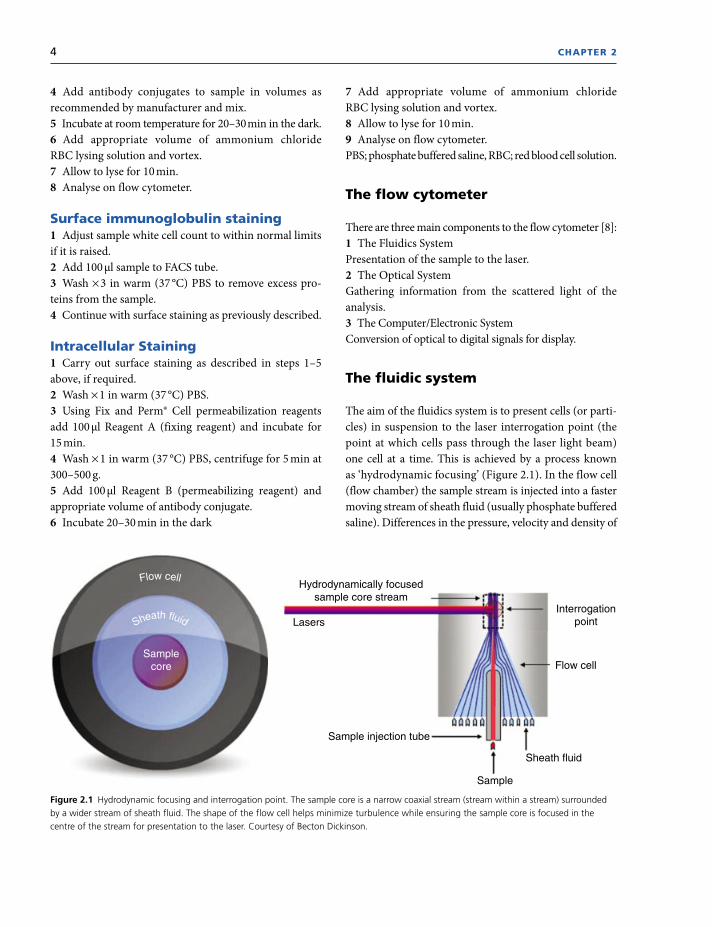
The fluidic system
The aim of the fluidics system is to present cells (or parti-
cles) in suspension to the laser interrogation point (the
point at which cells pass through the laser light beam)
one cell at a time. This is achieved by a process known
as ‘hydrodynamic focusing’ (Figure 2.1). In the flow cell
(flow chamber) the sample stream is injected into a faster
moving stream of sheath fluid (usually phosphate buffered
saline). Differences in the pressure, velocity and density of
Samplecore
Hydrodynamically focusedsample core stream
LasersInterrogation
point
Flow cell
Sheath fluid
Sample
Sample injection tube
Flow cell
Sheath fluid
Figure 2.1 Hydrodynamic focusing and interrogation point. The sample core is a narrow coaxial stream (stream within a stream) surrounded by a wider stream of sheath fluid. The shape of the flow cell helps minimize turbulence while ensuring the sample core is focused in the centre of the stream for presentation to the laser. Courtesy of Becton Dickinson.
Principles of Flow Cytometry 5
the two fluids prevent them from mixing. The flow cell is
designed so that at the laser interrogation point the two
streams are under pressure, focusing the sample stream in
the centre of the sheath fluid, forcing the cells into single
file before passing through the laser beam [3, 5, 6, 8].
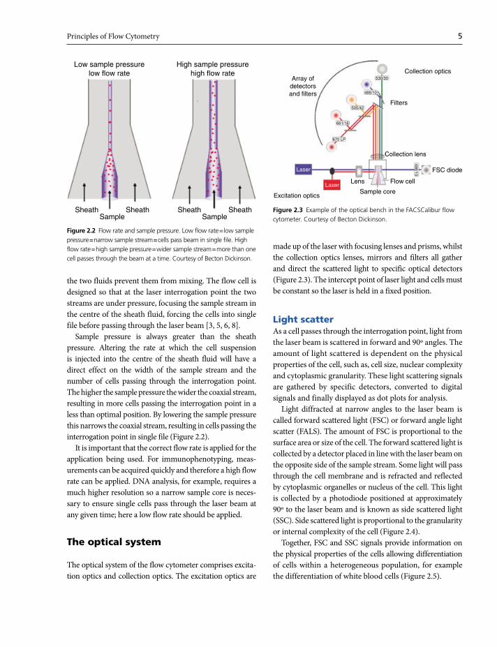
Sample pressure is always greater than the sheath
pressure. Altering the rate at which the cell suspension
is injected into the centre of the sheath fluid will have a
direct effect on the width of the sample stream and the
number of cells passing through the interrogation point.
The higher the sample pressure the wider the coaxial stream,
resulting in more cells passing the interrogation point in a
less than optimal position. By lowering the sample pressure
this narrows the coaxial stream, resulting in cells passing the
interrogation point in single file (Figure 2.2).
It is important that the correct flow rate is applied for the
application being used. For immunophenotyping, meas-
urements can be acquired quickly and therefore a high flow
rate can be applied. DNA analysis, for example, requires a
much higher resolution so a narrow sample core is neces-
sary to ensure single cells pass through the laser beam at
any given time; here a low flow rate should be applied.
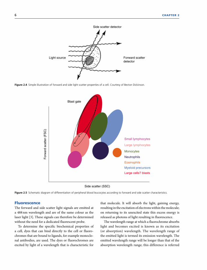
The optical system
The optical system of the flow cytometer comprises excita-
tion optics and collection optics. The excitation optics are
made up of the laser with focusing lenses and prisms, whilst
the collection optics lenses, mirrors and filters all gather
and direct the scattered light to specific optical detectors
(Figure 2.3). The intercept point of laser light and cells must
be constant so the laser is held in a fixed position.
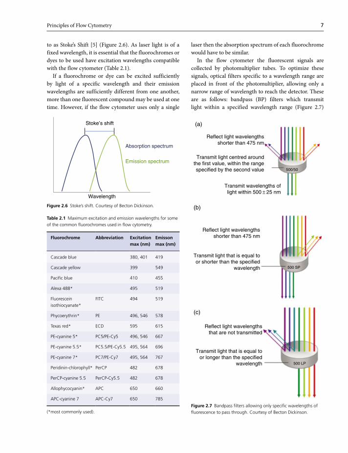
Light scatterAs a cell passes through the interrogation point, light from
the laser beam is scattered in forward and 90º angles. The
amount of light scattered is dependent on the physical
properties of the cell, such as, cell size, nuclear complexity
and cytoplasmic granularity. These light scattering signals
are gathered by specific detectors, converted to digital
signals and finally displayed as dot plots for analysis.
Light diffracted at narrow angles to the laser beam is
called forward scattered light (FSC) or forward angle light
scatter (FALS). The amount of FSC is proportional to the
surface area or size of the cell. The forward scattered light is
collected by a detector placed in line with the laser beam on
the opposite side of the sample stream. Some light will pass
through the cell membrane and is refracted and reflected
by cytoplasmic organelles or nucleus of the cell. This light
is collected by a photodiode positioned at approximately
90º to the laser beam and is known as side scattered light
(SSC). Side scattered light is proportional to the granularity
or internal complexity of the cell (Figure 2.4).
Together, FSC and SSC signals provide information on
the physical properties of the cells allowing differentiation
of cells within a heterogeneous population, for example
the differentiation of white blood cells (Figure 2.5).
Low sample pressurelow flow rate
Sheath SheathSample
Sheath SheathSample
High sample pressurehigh flow rate
Figure 2.2 Flow rate and sample pressure. Low flow rate = low sample pressure = narrow sample stream = cells pass beam in single file. High flow rate = high sample pressure = wider sample stream = more than one cell passes through the beam at a time. Courtesy of Becton Dickinson.
Figure 2.3 Example of the optical bench in the FACSCalibur flow cytometer. Courtesy of Becton Dickinson.
Array ofdetectorsand filters
Collection optics
Collection lens
Filters
530/30
488/10
488/10
505/42
661/16
670 LP
Laser
Laser
FSC diode
Flow cell
Sample core
Lens
Excitation optics
6 CHAPTER 2
Side scatter detector
Forward scatterdetector
Light source
Figure 2.4 Simple illustration of forward and side light scatter properties of a cell. Courtesy of Becton Dickinson.
For
war
d sc
atte
r (F
SC
)
Side scatter (SSC)
Small lymphocytes
Large lymphocytes
Monocytes
Neutrophils
Eosinophils
Myeloid precursors
Large cells? blasts
Blast gateate
Figure 2.5 Schematic diagram of differentiation of peripheral blood leucocytes according to forward and side scatter characteristics.
FluorescenceThe forward and side scatter light signals are emitted at
a 488 nm wavelength and are of the same colour as the
laser light [3]. These signals can therefore be determined
without the need for a dedicated fluorescent probe.
To determine the specific biochemical properties of
a cell, dyes that can bind directly to the cell or fluoro-
chromes that are bound to ligands, for example monoclo-
nal antibodies, are used. The dyes or fluorochromes are
excited by light of a wavelength that is characteristic for
that molecule. It will absorb the light, gaining energy,
resulting in the excitation of electrons within the molecule;
on returning to its unexcited state this excess energy is
released as photons of light resulting in fluorescence.
The wavelength range at which a fluorochrome absorbs
light and becomes excited is known as its excitation
(or absorption) wavelength. The wavelength range of
the emitted light is termed its emission wavelength. The
emitted wavelength range will be longer than that of the
absorption wavelength range; this difference is referred
Principles of Flow Cytometry 7
to as Stoke’s Shift [5] (Figure 2.6). As laser light is of a
fixed wavelength, it is essential that the fluorochromes or
dyes to be used have excitation wavelengths compatible
with the flow cytometer (Table 2.1).
If a fluorochrome or dye can be excited sufficiently
by light of a specific wavelength and their emission
wavelengths are sufficiently different from one another,
more than one fluorescent compound may be used at one
time. However, if the flow cytometer uses only a single
laser then the absorption spectrum of each fluorochrome
would have to be similar.
In the flow cytometer the fluorescent signals are
collected by photomultiplier tubes. To optimize these
signals, optical filters specific to a wavelength range are
placed in front of the photomultiplier, allowing only a
narrow range of wavelength to reach the detector. These
are as follows: bandpass (BP) filters which transmit
light within a specified wavelength range (Figure 2.7)
Stoke’s shift
Wavelength
Absorption spectrum
Emission spectrum
Figure 2.6 Stoke’s shift. Courtesy of Becton Dickinson.
Table 2.1 Maximum excitation and emission wavelengths for some of the common fluorochromes used in flow cytometry.
Fluorochrome Abbreviation Excitation max (nm)
Emisson max (nm)
Cascade blue 380, 401 419
Cascade yellow 399 549
Pacific blue 410 455
Alexa 488* 495 519
Fluorescein isothiocyanate*
FITC 494 519
Phycoerythrin* PE 496, 546 578
Texas red* ECD 595 615
PE-cyanine 5* PC5/PE-Cy5 496, 546 667
PE-cyanine 5.5* PC5.5/PE-Cy5.5 495, 564 696
PE-cyanine 7* PC7/PE-Cy7 495, 564 767
Peridinin-chlorophyll* PerCP 482 678
PerCP-cyanine 5.5 PerCP-Cy5.5 482 678
Allophycocyanin* APC 650 660
APC-cyanine 7 APC-Cy7 650 785
(*most commonly used).Figure 2.7 Bandpass filters allowing only specific wavelengths of fluorescence to pass through. Courtesy of Becton Dickinson.
(a)
Reflect light wavelengthsshorter than 475 nm
Transmit light centred aroundthe first value, within the rangespecified by the second value
Transmit wavelengths oflight within 500 ± 25 nm
500/50
(b)
Reflect light wavelengthsshorter than 475 nm
Transmit light that is equal toor shorter than the specified
wavelength 500 SP
(c)
Reflect light wavelengthsthat are not transmitted
Transmit light that is equal toor longer than the specified
wavelength 500 LP
8 CHAPTER 2
(a); shortpass (SP) filters (b) which transmit light with
wavelengths equal to or shorter than specified; longpass
(LP) filters (c) which transmit light with wavelengths
equal to or longer than specified.
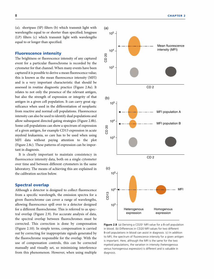
Fluorescence intensityThe brightness or fluorescence intensity of any captured
event for a particular fluorochrome is recorded by the
cytometer for that channel. When many events have been
captured it is possible to derive a mean fluorescence value;
this is known as the mean fluorescence intensity (MFI)
and is a very important characteristic that should be
assessed in routine diagnostic practice (Figure 2.8a). It
relates to not only the presence of the relevant antigen,
but also the strength of expression or integrity of that
antigen in a given cell population. It can carry great sig-
nificance when used in the differentiation of neoplastic
from reactive and normal cell populations. Fluorescence
intensity can also be used to identify dual populations and
allow subsequent directed gating strategies (Figure 2.8b).
Some cell populations can show a spectrum of expression
of a given antigen, for example CD13 expression in acute
myeloid leukaemia, so care has to be used when using
MFI data without paying attention to the plot
(Figure 2.8c). These patterns of expression can be impor-
tant in diagnosis.
It is clearly important to maintain consistency in
fluorescence intensity data, both on a single cytometer
over time and between different cytometers in the same
laboratory. The means of achieving this are explained in
the calibration section below.
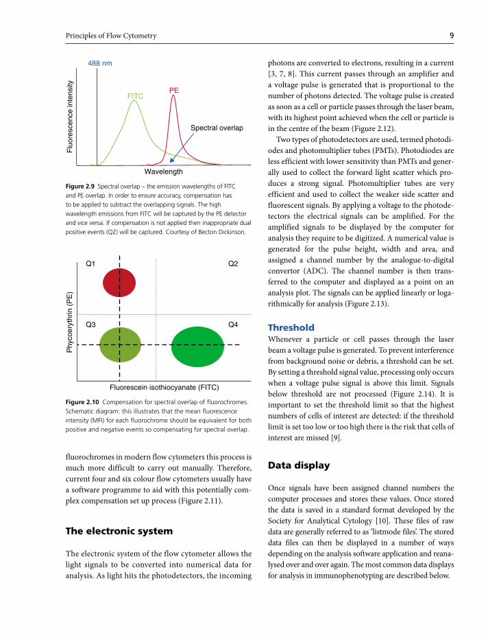
Spectral overlapAlthough a detector is designed to collect fluorescence
from a specific wavelength, the emission spectra for a
given fluorochrome can cover a range of wavelengths,
allowing fluorescence spill over to a detector designed
for a different fluorochrome. This is referred to as spec-
tral overlap (Figure 2.9). For accurate analysis of data,
the spectral overlap between fluorochromes must be
corrected. This correction is done by compensation
(Figure 2.10). In simple terms, compensation is carried
out by correcting for inappropriate signals generated by
the fluorochrome responsible for the overlap. With the
use of compensation controls, this can be corrected
manually and visually set, so minimizing interference
from this phenomenon. However, when using multiple
Figure 2.8 (a) Deriving a CD20+ MFI value for a B-cell population in blood. (b) Differences in CD20 MFI values for two different B-cell populations in blood can assist in diagnosis. (c) In addition to MFI, the spectrum of fluorescence intensity for a given antigen is important. Here, although the MFI is the same for the two myeloid populations, the variation in intensity (heterogenous versus homogenous expression) is different and is valuable in diagnosis.
CD
20
CD 2
(a)
105
104
103
Mean fluorescence intensity (MFI)
CD
20
CD 2
105
104
103
MFI population A
MFI population B
(b)
CD
13
105
104
103
MFI
Heterogenousexpression
Homogenousexpression
(c)
Principles of Flow Cytometry 9
fluorochromes in modern flow cytometers this process is
much more difficult to carry out manually. Therefore,
current four and six colour flow cytometers usually have
a software programme to aid with this potentially com-
plex compensation set up process (Figure 2.11).
The electronic system
The electronic system of the flow cytometer allows the
light signals to be converted into numerical data for
analysis. As light hits the photodetectors, the incoming
photons are converted to electrons, resulting in a current
[3, 7, 8]. This current passes through an amplifier and
a voltage pulse is generated that is proportional to the
number of photons detected. The voltage pulse is created
as soon as a cell or particle passes through the laser beam,
with its highest point achieved when the cell or particle is
in the centre of the beam (Figure 2.12).
Two types of photodetectors are used, termed photodi-
odes and photomultiplier tubes (PMTs). Photodiodes are
less efficient with lower sensitivity than PMTs and gener-
ally used to collect the forward light scatter which pro-
duces a strong signal. Photomultiplier tubes are very
efficient and used to collect the weaker side scatter and
fluorescent signals. By applying a voltage to the photode-
tectors the electrical signals can be amplified. For the
amplified signals to be displayed by the computer for
analysis they require to be digitized. A numerical value is
generated for the pulse height, width and area, and
assigned a channel number by the analogue-to- digital
convertor (ADC). The channel number is then trans-
ferred to the computer and displayed as a point on an
analysis plot. The signals can be applied linearly or loga-
rithmically for analysis (Figure 2.13).
ThresholdWhenever a particle or cell passes through the laser
beam a voltage pulse is generated. To prevent interference
from background noise or debris, a threshold can be set.
By setting a threshold signal value, processing only occurs
when a voltage pulse signal is above this limit. Signals
below threshold are not processed (Figure 2.14). It is
important to set the threshold limit so that the highest
numbers of cells of interest are detected: if the threshold
limit is set too low or too high there is the risk that cells of
interest are missed [9].
Data display
Once signals have been assigned channel numbers the
computer processes and stores these values. Once stored
the data is saved in a standard format developed by the
Society for Analytical Cytology [10]. These files of raw
data are generally referred to as ‘listmode files’. The stored
data files can then be displayed in a number of ways
depending on the analysis software application and reana-
lysed over and over again. The most common data displays
for analysis in immunophenotyping are described below.
FITCPE
488 nm
Spectral overlap
Wavelength
Flu
ores
cenc
e in
tens
ity
Figure 2.9 Spectral overlap – the emission wavelengths of FITC and PE overlap. In order to ensure accuracy, compensation has to be applied to subtract the overlapping signals. The high wavelength emissions from FITC will be captured by the PE detector and vice versa. If compensation is not applied then inappropriate dual positive events (Q2) will be captured. Courtesy of Becton Dickinson.
Fluorescein isothiocyanate (FITC)
Q1 Q2
Q3 Q4
Phy
coer
ythr
in (
PE
)
Figure 2.10 Compensation for spectral overlap of fluorochromes. Schematic diagram: this illustrates that the mean fluorescence intensity (MFI) for each fluorochrome should be equivalent for both positive and negative events so compensating for spectral overlap.

Figure 2.11 Compensation for spectral overlap of fluorochromes: illustrating a worked example.
(a) Correct compensation Accurate compensation allows for spectral overlap and generates discrete cell populations with equivalent MFI for both FITC (green values) and PE (red values) channels.
(b) Over compensation This encourages populations to be pulled down the axis for the relevant fluorochrome – too much subtraction collapses/skews the
events downward and the MFI values are different. If this is not corrected dual positive population may be missed.
(c) Under compensation This encourages populations to be pulled up the axis for the opposing fluorochrome – too little subtraction collapses/skews the events upward and the MFI values are different. This may lead to false dual positivity being reported.
105 Q1
Q3
FITC-A
Q2
Q4
0 102 103 104 105–165
104
PE
-A–7
7410
30
(a)
Population
Q1Q2Q3Q4
491,398
441,784
12,7865,330
173176
MeanFITC-A PE-A
Mean
105 Q1
Q3
FITC-A
Q2
Q4
0 102 103 104 105–445
104
PE
-A
–1,3
9110
30
(b)
–102
Population
Q1Q2Q3Q4
–2021,553
591,835
12,6851,539
217–109
MeanFITC-A PE-A
Mean
105 Q1
Q3
FITC-A
Q2
Q4
0 102 103 104 105–162
104
PE
-A–5
8710
30
(c)
Population
Q1Q2Q3Q4
1642,728
631,610
12,3992,598
238483
MeanFITC-A PE-A
Mean
Principles of Flow Cytometry 11
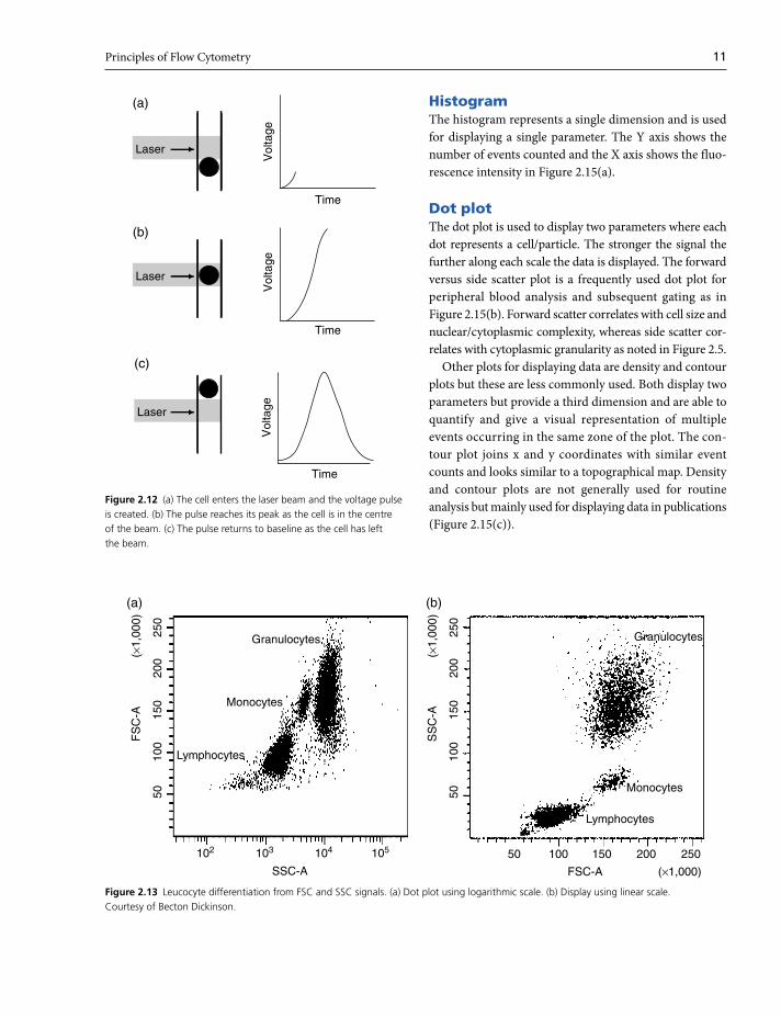
HistogramThe histogram represents a single dimension and is used
for displaying a single parameter. The Y axis shows the
number of events counted and the X axis shows the fluo-
rescence intensity in Figure 2.15(a).
Dot plotThe dot plot is used to display two parameters where each
dot represents a cell/particle. The stronger the signal the
further along each scale the data is displayed. The forward
versus side scatter plot is a frequently used dot plot for
peripheral blood analysis and subsequent gating as in
Figure 2.15(b). Forward scatter correlates with cell size and
nuclear/cytoplasmic complexity, whereas side scatter cor-
relates with cytoplasmic granularity as noted in Figure 2.5.
Other plots for displaying data are density and contour
plots but these are less commonly used. Both display two
parameters but provide a third dimension and are able to
quantify and give a visual representation of multiple
events occurring in the same zone of the plot. The con-
tour plot joins x and y coordinates with similar event
counts and looks similar to a topographical map. Density
and contour plots are not generally used for routine
analysis but mainly used for displaying data in publications
(Figure 2.15(c)).
Figure 2.12 (a) The cell enters the laser beam and the voltage pulse is created. (b) The pulse reaches its peak as the cell is in the centre of the beam. (c) The pulse returns to baseline as the cell has left the beam.
Laser
Vol
tage
Time
(a)
LaserV
olta
ge
Time
(b)
Laser
Vol
tage
Time
(c)
Figure 2.13 Leucocyte differentiation from FSC and SSC signals. (a) Dot plot using logarithmic scale. (b) Display using linear scale. Courtesy of Becton Dickinson.
Lymphocytes
Monocytes
Granulocytes 250
(×1,
000)
200
150
FS
C-A
100
50
102 103
SSC-A
105104
(a)
Lymphocytes
Monocytes
Granulocytes250
(×1,
000)
(×1,000)FSC-A
200
150
SS
C-A
100
50
50 100 150 200 250
(b)

12 CHAPTER 2
GatingGating refers to the ability to isolate single populations of
interest within a heterogeneous sample. As flow cytome-
ters are capable of analysing thousands of cells per second,
gating allows analysis to be restricted to a subpopulation
of cells without having to isolate them from a mixed sam-
ple prior to analysis [5]. As previously shown in Figure 2.5,
subpopulations of leucocytes can be identified according
Vol
tage
Threshold
Figure 2.14 The principle of setting a threshold voltage. Courtesy of Becton Dickinson.
Figure 2.15 (a) Histogram plot showing CD2 expression of peripheral blood lymphocytes. (b) Dot plot using a forward scatter (FSC) versus side scatter (SSC) analysis. (c) Contour plot (left) and density plot (right) of the same forward scatter (FSC) versus side scatter (SSC) analysis.
9080
7060
P1
(a)
Cou
nt
5040
3020
100
0–165CD2 FITC-A
102 103 104 105
250
(×1,
000)
200
150
FS
C-A
100
50
102 103
SSC-A
105104
(b)
250
(×1,
000)
200
150
FS
C-A
100
50
102 103
SSC-A
105104
250
(×1,
000)
200
150
FS
C-A
100
50
102 103
SSC-A
105104
(c)

Principles of Flow Cytometry 13
to their light scatter properties. If left ungated, then non-
specific fluorescence from monocytes and neutrophils
will be seen on the analysis plot. However, by drawing a
gate (or region) around the lymphocyte population the
fluorescent properties of only lymphocytes can be dis-
played, making analysis much more specific (Figure 2.16).
The orientation of populations of cells in a FSC versus
SSC light scatter plot is the simplest method for gating.
It has the advantage that dead cells or debris can be
excluded from the analysis but the disadvantage of being
unable to discriminate between cells with similar light
scatter properties.
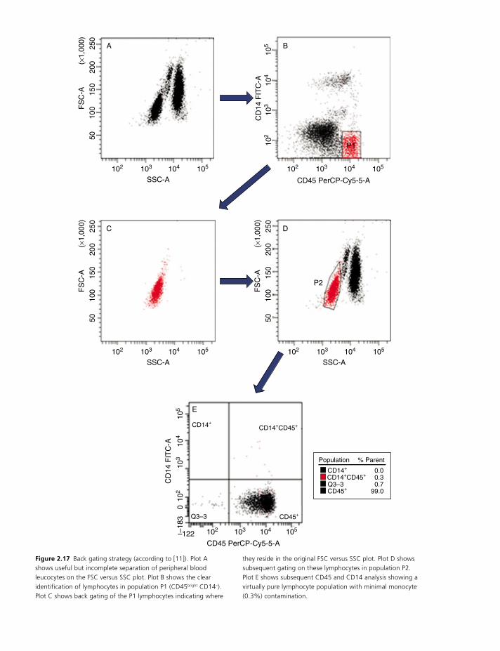
Lack of discrimination according to light scatter
behaviour can be overcome by ‘back gating’. This is a
strategy that can be used to identify a population of
cells for analysis while excluding contamination by
other cell populations, for example monocytes being
included in the lymphocyte gate. This was first
described in 1990 [11]: by staining cells with CD45 (all
normal leucocytes are CD45+) and CD14, (monocytes
are CD14+, lymphocytes CD14–) a dual parameter dot
plot of CD45 versus CD14 is created. By drawing a gate
around the brightest CD45+ CD14– populations it is
then possible to identify the lymphocytes with minimal
monocyte contamination (Figure 2.17).
With the introduction of more monoclonal antibodies
in multiparameter flow cytometry it has become com-
mon to use specific cell surface antigen expression as a
gating parameter as a means of identifying the cells of
interest within a heterogeneous population. By using
fluorescence along with side scatter as a gating parame-
ter this can provide the interpreter with a specific pheno-
type of these cells. For example, if CD19 was used to
isolate B lymphocytes from the T lymphocytes the
resulting information would only be relevant to the
B-lymphocyte population within the sample. This same
principle can be applied to identifying blasts within a
leukaemic sample (Figure 2.18).
Another common gating strategy utilizes CD45 as
the fluorescent parameter. CD45 is a common surface
antigen expressed on leucocytes with differing levels of
fluorescence intensity, but is not expressed by erythroid
or non-haematological cells. Lymphocytes can be easily
identified by their higher CD45 staining intensity than
that of monocytes and granulocytes. Due to this differ-
ence in fluorescence intensity between cell types, along
with side scatter properties, CD45 can be a useful gating
parameter for identifying leucocytes of different lineages
and degrees of maturation [12] (Figure 2.19).
It is possible to apply multiple gates; several sequential
gates can be set on different parameters and analysed
simultaneously. In the clinical setting examples of this
include the enumeration of CD34+ cells in peripheral
blood or peripheral blood stem cell collections, and
250
200
150
FS
C-A
100
50
102 103 104
SSC-A
Lymphocytes(×
1,00
0)
105 102
105
104
103
0
0
Q3
Q2CD19
CD2
–156
–770
CD
19 P
E-A
103 104
CD2 FITC-A105
Population
CD19Q2Q3CD2
9.00.3
19.771.1
% Parent
Figure 2.16 A FSC/SCC plot showing gate around lymphocytes and a dot plot showing only parameters related to the gated region.
250
200
150
FS
C-A
(×1,
000)
100
50
102 103
SSC-A
A B
C
E
D
104 105
250
200
150
FS
C-A
(×1,
000)
100
50
102 103
SSC-A104 105
250
200
150
FS
C-A
(×1,
000)
100
50
102 103
SSC-A
P2
104 105
102 103
CD45 PerCP-Cy5-5-A
P1
104 105
105
104
103
CD
14 F
ITC
-A10
2
102 103
CD45 PerCP-Cy5-5-A
104 105
105
104
103
CD
14 F
ITC
-A
102
0–1
83
–122
CD14+CD14+CD45+
Q3–3 CD45+
Population
CD14+
CD14+CD45+
Q3–3CD45+
0.00.30.7
99.0
% Parent
Figure 2.17 Back gating strategy (according to [11]). Plot A shows useful but incomplete separation of peripheral blood leucocytes on the FSC versus SSC plot. Plot B shows the clear identification of lymphocytes in population P1 (CD45bright CD14–). Plot C shows back gating of the P1 lymphocytes indicating where
they reside in the original FSC versus SSC plot. Plot D shows subsequent gating on these lymphocytes in population P2. Plot E shows subsequent CD45 and CD14 analysis showing a virtually pure lymphocyte population with minimal monocyte (0.3%) contamination.

Principles of Flow Cytometry 15
CD4+ helper T-cell numbers from the total T-lymphocyte
population [13, 14] (Figure 2.20).
Instrument set-up and quality controlTo ensure the accuracy and precision of the data generated,
particularly in the clinical laboratory, the performance of
the flow cytometer must be rigorously monitored and
controlled. Although most instrument calibration is car-
ried out during installation, it is good laboratory practice
for the flow lab to establish a robust internal quality
control (IQC) programme. This will ensure that the flow
cytometer performs to its expected standard. This can be
done through the use of commercial standards and con-
trol materials. The term ‘standard’ usually refers to a sus-
pension of microbeads/particles which do not require
further preparation and are generally used to set up or
calibrate the instrument. Control material is different in
that they are usually analytes, for example fixed whole
blood cells that have pre-determined values and require
preparation in a similar way to patient samples [15].
102
105
104
103
102
CD
19 A
PC
-A
103 104
SSC-A
CD19 positive cells
105 102
105
104
103
102
CD
34 A
PC
-A
103 104
SSC-A
CD34 positive cells
105
Figure 2.18 Illustration of gating strategy using fluorescence versus SSC to isolate the cells of interest. B lymphocytes are identified using CD19 (left) whilst CD34 (right) is used to identify blasts.
CD
45
Side scatter
103
102
101
LymphocytesMonocytesNeutrophilsPromyelocytesMeta/MyelocytesLymphoblastsMyeloblasts/MonoblastsNucleated Erythroid Cells
Neg
Dim
Bright
Figure 2.19 CD45 plot leucocyte lineage and maturation.

16 CHAPTER 2
The microbead standards can be classified into four
categories [15]:
Type 0 (certified blank): these beads are approximately
the same size as a lymphocyte, with no added fluorescent
dye. They have a fluorescence signal lower than the
autofluorescence of unstained peripheral blood lympho-
cytes, helping to set the threshold level so that there is no
interference from noise in the immunophenotyping assay.
Type I (alignment beads): these are designed for optical
alignment of the flow cytometer. They are subclassified
according to size into type Ia (smaller than a lymphocyte)
250
200
150
SS
C-A
( ×1,
000)
100
50
102 103
CD45 FITC-A
P1
104 105
250
200
150
SS
C-A
(×1,
000)
100
50
102 103
CD45 FITC-A
P3
Tube: 1
PopulationAll events
P1P2
P3
104 105
250
200
150
SS
C-A
(×1,
000)
100
50
102 103
CD34 PE-A
P2
104 105
Figure 2.20 Simplified example of sequential gating used in the ISHAGE protocol for absolute CD34 enumeration. A plot displaying SSC versus CD45 FITC fluorescence has a gate P1 drawn around all positive cells excluding noise/debris. Everything within P1 is displayed on a second plot, SSC versus anti-CD34 PE. A gate is drawn around the positive cells in gate P2 which in turn are displayed on another SSC versus CD45 FITC and a gate drawn around the discrete group of cells with moderate FITC fluorescence intensity and low SSC
properties, gate P3. By following the population hierarchy the gating sequence can be understood. The cells within the P3 gate are also found in P1 and P2 regions. This sequential gating process effectively purifies the CD34+ population and excludes rogue cells. Gates can be set during acquisition (real time) or post acquisition. Either way since the computer saves the files (listmode data), repeated analysis can be carried out with different gating strategies being applied an infinite number of times without affecting the original file.

Principles of Flow Cytometry 17
and type Ib (equivalent size to a lymphocyte). Since the
optical system of most flow cytometers is fixed it is prefer-
able that the optical alignment is carried out by trained
engineers. The use of alignment beads by the user is
mainly in the setting up of cell sorters.
Type II (reference beads): these have bright fluorescence
intensity and are subclassified into type IIa, IIb and IIc
according to their excitation and emission spectra and
whether they have antibody binding capacity. Type IIa
and IIb beads are labelled with broad spectra or specific
C
300
250
200
150
Cou
nt
100
500
102
PopulationP2 1,120 11.2 33,142
#Events %ParentAPC-AMean
103
APC-A
104 105
P2
A B
250
200
150
SS
C-A
( ×1,
000)
100
50
250200150
FSC-A (×1,000)
10050
250
200
150
SS
C-A
(×1,
000)
100
50
250200150
FSC-A (×1,000)
10050
P1
Figure 2.21 Example of daily IQC using eight peak rainbow beads for instrument stability. Plot A: This shows gating on P1 around singlet beads to exclude doublets. Plot B: This indicates that FSC – height versus FSC – area are proportional. Plot C: The brightest peak is gated (P2) and the MFI is displayed. There should be minimal change in MFI between each analysis.
18 CHAPTER 2
fluorochromes respectively. Type IIc beads are unlabelled,
allowing binding with the same antibody conjugate used
to label the cells.
Type III (calibration beads): these beads are equivalent in
size to lymphocytes but have varying fluorescence inten-
sity, ranging from dim to bright. They share the same
properties as type IIa, IIb and IIc beads. These beads are
used in quantitative flow cytometry where a calibration
curve is required to determine the antibody binding
capacity of the cell. This analysis provides a measure of
the amount of cell surface antigen present on an individ-
ual cell [15, 16] and is not normally required for routine
diagnostic purposes.
Type IIc and IIIc can be labelled with specific antibody
conjugates. As this is the principle applied in immu-
nophenotyping, they are useful for setting spectral over-
lap or compensation values. However, compensation
should be validated using biological samples stained with
the specific antibody conjugate of interest.
To ensure unified set up, it is recommended that a win-
dow of analysis be determined. This can be achieved
using type IIb reference standards and placing beads in
specified target channels. Daily monitoring of type IIb
reference beads reliably monitors reproducibility of the
flow cytometer. If the laboratory has more than one flow
cytometer it is important to ensure that all instruments
are standardized in the same manner [16].
The IQC protocol for the laboratory should be
performed on a daily basis. It is essential that the data
generated by the reference beads is recorded and
reviewed frequently to verify instrument per-
formance (Figure 2.21).
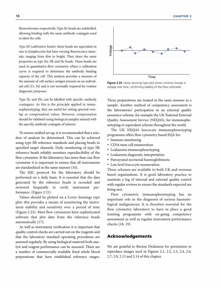
Values should be plotted on a Levey–Jennings type
plot; this provides a means of monitoring the instru-
ment stability and sensitivity over a period of time
(Figure 2.22). Most flow cytometers have sophisticated
software that plot data from the reference beads
automatically [17].
As well as instrument verification it is important that
quality control checks are carried out on the reagents and
that the laboratory standard operating procedures are
assessed regularly. By using biological material both ana-
lyst and reagent performance can be assessed. There are
a number of commercially available fixed whole blood
preparations that have established reference ranges.
These preparations are treated in the same manner as a
sample. Another method of competency assessment is
the laboratories’ participation in an external quality
assurance scheme, for example the UK National External
Quality Assessment Service (NEQAS), for immunophe-
notyping or equivalent scheme throughout the world.
The UK NEQAS leucocyte immunophenotyping
programme offers flow cytometry based EQA for:
Immune monitoring
CD34 stem cell enumeration
Leukaemia immunophenotyping
Leukaemia diagnostic interpretation
Paroxysmal nocturnal haemoglobinuria
Low level leucocyte enumeration.
These schemes are available to both UK and overseas
based organizations. It is good laboratory practice to
maintain a log of internal and external quality control
with regular reviews to ensure the standards expected are
being met.
Flow cytometric immunophenotyping has an
important role in the diagnosis of serious haemato-
logical malignancies. It is therefore essential for the
flow cytometry laboratory to have in place a good
training programme with on-going competency
assessment as well as regular instrument performance
checks [18, 19].
Acknowledgements
We are grateful to Becton Dickinson for permission to
reproduce images used in Figures 2.1, 2.2, 2.3, 2.4, 2.6,
2.7, 2.9, 2.13 and 2.14 of this chapter.
Vol
tage
Time
Figure 2.22 Levey–Jennings type plot shows minimal change in voltage over time, confirming stability of the flow cytometer.

Principles of Flow Cytometry 19
References
1 Brown M, Wittwer C. Flow cytometry: principles and clini-
cal applications in hematology. Clin Chem 2000, 46(8 Pt 2):
1221–9.
2 Robinson JP. Flow Cytometry. Encyclopedia of Biomaterials
and Biomedical Engineering. 2004. pp. 630–40.
3 Givan AL. Principles of flow cytometry: an overview.
Methods Cell Biol 2001, 63:19–50.
4 Delude RL. Flow cytometry. Critical Care Medicine 2005,
33(Suppl): S426–S8.
5 McCoy JP, Jr. Basic principles of flow cytometry. Hematol
Oncol Clin North Am 2002, 16(2): 229–43.
6 Nunez R. Flow cytometry: principles and instrumentation.
Curr Issues Mol Biol 2001, 3(2): 39–45.
7 Shapiro HM. Practical Flow Cytometry, 4th edn. 2003. Wiley-
Liss, New York.
8 Becton Dickinson Biosciences. Introduction to Flow Cyto-
metry: A Learning Guide. 2000. San Jose: Becton Dickinson
Biosciences.
9 Wood JC. Principles of gating. Curr Protoc Cytom 2001,
Chapter 1: Unit 18.
10 Data file standard for flow cytometry. Data File Standards
Committee of the Society for Analytical Cytology. Cytometry
1990, 11(3): 323–32.
11 Loken MR, Brosnan JM, Bach BA, Ault KA. Establishing
optimal lymphocyte gates for immunophenotyping by flow
cytometry. Cytometry 1990, 11(4): 453–9.
12 Stelzer GT, Shults KE, Loken MR. CD45 gating for routine
flow cytometric analysis of human bone marrow specimens.
Ann N Y Acad Sci 1993, 677: 265–80.
13 Keeney M, Chin-Yee I, Weir K, Popma J, Nayar R,
Sutherland DR. Single platform flow cytometric absolute
CD34+ cell counts based on the ISHAGE guidelines. Inter-
national Society of Hematotherapy and Graft Engineering.
Cytometry 1998, 34(2): 61–70.
14 Mandy FF, Nicholson JK, McDougal JS. Guidelines for
performing single-platform absolute CD4+ T-cell deter-
minations with CD45 gating for persons infected with
human immunodeficiency virus. Centers for disease control
and prevention. MMWR Recomm Rep. 2003, 52(RR-2):
1–13.
15 Schwartz A, Marti GE, Poon R, Gratama JW, Fernandez-
Repollet E. Standardizing flow cytometry: a classification
system of fluorescence standards used for flow cytometry.
Cytometry 1998, 33(2): 106–14.
16 Stelzer GT, Marti G, Hurley A, McCoy P, Jr., Lovett EJ,
Schwartz A. US-Canadian Consensus recommendations on
the immunophenotypic analysis of hematologic neoplasia by
flow cytometry: standardization and validation of laboratory
procedures. Cytometry 1997, 30(5): 214–30.
17 Ormerod MG. Flow Cytometry: A Practical Approach, 3rd
edn. Oxford University Press, Oxford.
18 Owens MA, Vall HG, Hurley AA, Wormsley SB. Validation
and quality control of immunophenotyping in clinical flow
cytometry. J Immunol Methods 2000, 243(1–2): 33–50.
19 Greig B, Oldaker T, Warzynski M, Wood B. 2006 Bethesda
International Consensus recommendations on the immu-
nophenotypic analysis of hematolymphoid neoplasia by
flow cytometry: recommendations for training and educa-
tion to perform clinical flow cytometry. Cytometry B Clin
Cytom 2007, 72(Suppl 1): S23–33.