2. CLASSICAL ELECTRODYNAMICS IN GEOMAGNETISM

As we turn to the geomagnetic part of this course we will apply many of the same mathematical tools as

are used in studying Earth’s gravitational potential. However, instead of Newton’s law, the fundamental

physics are described by the equations of classical electrodynamics. This chapter starts with Helmholtz’s

theorem, Maxwell’s equations, and Ohm’s law in a moving medium, and motivates the equations that are

used in static geomagnetic field modeling. Much of the material covered here is to be found in Chapter 2 of

Foundations; a less advanced treatment is given in Chapters 2 and 4 of Blakely’s book on Potential Theory.

2:1 Helmholtz’s Theorem and Maxwell’s Equations

The universe of classical electrodynamics begins with a vacuum containing matter solely in the form of

electric charges, possibly in motion, and electric and magnetic fields. We can detect the presence of these

fields by the forces they exert on a moving point charge q. If the charge q is located at position r at time t

and moves with velocity v relative to an inertial frame, then

f = q[E(r, t) + v! B(r, t)]. (3)

This expression allows us in principle to measure the electric and magnetic fields using a moving charge as

a detector in an inertial reference frame.

Maxwell’s equations provide the curl and divergence of the electric fields and magnetic fields in terms of

other things. The reason this is useful is that Helmholtz’s Theorem tells us that if we know the curl and

the divergence of a vector field, we can explicitly calculate the field itself, and furthermore, the curl and

the divergence represent sources for the field, essentially creating the field. Here is Helmholtz’s theorem.

A vector field F in R3 which is continuously differentiable (except for jump discontinuities across certain

surfaces) is uniquely determined by its divergence, its curl and jump discontinuities if it approaches 0 at

infinity. The field can be written as the sum of two parts

F = "#V + #! A (4)

where V is called a scalar potential and A a vector potential. These two potentials can be explicitly computed

from the following two integrals:

V (r) =1

4!

!d3s # · F(s)

|r " s| (5)

A(r) =1

4!

!d3s #! F(s)

|r " s| . (6)

9

What these two equations state is that the field F is generated by two kinds of sources: one is the divergence

of F, the other its curl. Recall that in classical gravity, the gravitational potential V is generated by matter

density " and we see this through:

V (r) = "G

!d3s "(s)

|r" s| . (6a)

But this is just equation (5), because of Poisson’s equation, #2V = 4!G" and the fact that here F = g =

"#V . Helmholtz tells us that if there is no divergence or curl anywhere in space, then F must vanish, again

confirming that# · F and#!F are the sources of the field. Now back to Maxwell’s equations in a vacuum.

Recall the universe we are operating in comprises an infinite vacuum containing electrical charges, repre-

sented by a local density ", which may be moving, and hence generating electric current, represented by a

local current density J. Here are Maxwell’s equations:

#! E = "#tB (7)

# · E = "/$0 (8)

#! B = µ0(J + $0#tE) (9)

# · B = 0 (10)

where " is charge density (in SI units coulombs/m3), J is current density (amperes/m2), µ0 is permeability

of vacuum (4!! 10"7 henries/m), $0 is capacitivity of vacuum (107/4!c2 farads/m); B is in teslas, and E is

in volts/m. The quantities µ0 and $0 are exactly defined constants of the SI measurement conventions; the

quantity c is the velocity of light in a vacuum, which is also an exact number in SI. Notice I have introduced

the somewhat unconventional, streamlined notation for time derivative: #/#t = #t.

Viewed from the perspective of Helmholtz’s Theorem we see that the Maxwell equations (7) and (8) tell

us how a magnetic field is generated (by changing magnetic fields — Faraday’s law) or by the presence of

electric charges (Coulomb’s law); and equation (9) says we can generate a magnetic field by a combination

of moving charges (Ampere’s law) and by changing the electric field in time (Maxwell’s discovery, which

does not have the word law associated with it). Equation (10) says there are no isolated magnetic charges,

that is, no magnetic monopoles.

2:2 The Static Case for Geomagnetic Field Modeling

For some purposes we can neglect time variation in geomagnetic processes and imagine a system of

stationary charges and steady current flows. Many geomagnetic phenomena take place over long time

10

scales and certainly for the purposes of modeling the present geomagnetic field this seems like a reasonable

approximation. In (7), the first of the Maxwell equations, we set #tB = 0; then the curl of the electric field

vanishes. Making use of this in (4) and (6) we find that the electric field may be written as the gradient of a

scalar % (the electric potential). Thus

E = "#%. (11)

Putting this together with (8) and (5) we get #2% = ""/$0 (Poisson’s equation again, but notice the sign!)

and

%(r) =1

4!$0

!d3s "(s)

|r" s| . (12)

For the magnetic field it follows from# · B = 0 and (5),(4) that we can always write B = #!A. The vector

field A is known as the magnetic vector potential. Now if we specialize to the static case with #tE = 0, we

find from (9), and (6) that

A(r) =µ0

4!

!d3s J(s)

|r" s| . (13)

Again from (9) we have that J = #! B/µ0 and taking the divergence yields

# · J = 0. (14)

2:3 Constitutive Relations

Maxwell’s equations as written in (7)-(10) apply to a vacuum. When we need equations describing the

behavior of electromagnetic fields inside a material we require some mechanism for spatial averaging of

the charge and current distributions due to the atoms making up the material. This question is considered

in most courses on electromagnetism, and in Foundations. These lead us to a form of Maxwell’s equations

capable of describing field within various materials

#! E = "#tB (16)

$0# · E = " " # · P (17)

#! B/µ0 = (J + #tP + #!M + $0#tE) (18)

# · B = 0 (19)

where P and M are the electric polarization per unit volume and the magnetization, or magnetic polarization

per unit volume of the material. Physically what happens is that the presence of an electric field (for

simplicity) polarizes the material, causing charge separation. This introduces a large number of tiny electric

11

dipoles into the medium, quantified by the term P – this is simply the density of electric dipole moment

present in the material. If the dipole density were precisely constant, there would be no effect on E,

because the dipole fields would cancel on average (except at the ends of the specimen, where charges would

accumulate). But variations in the dipole density do cause electric fields – this is seen in the fact that the term

in the modified equations is # · P. The magnetic effect is similar, but more complicated because electrons’

intrinsic magnetic moments and their motions within atoms cause magnetic fields.

The solution of Maxwell’s equations for E and B in a material thus requires knowledge of J, P and M and

these in turn depend on the way the material responds to the fields. These are called the constitutive relations

for the material and are often determined by E and B themselves. They are not fundamental like Maxwell’s

equations, but are the result of empirical observations and experiments done on different materials. The

simplest possible behavior is linear. For example for many materials over a wide range of field values, we

find

J = &E (20)

P = $0'EE (21)

M = (B/µ0 (22)

where &, 'E and ( are constants. We can recognize & as the electrical conductivity, 'E as the electrical

susceptibility, and ( as a kind of magnetic susceptibility.

We can simplify Maxwell’s equations by defining new fields H and D,

D = $0E + P (23)

H = B/µ0 " M. (24)

D is called the electric displacement vector. H has traditionally been called the magnetic field vector, while

B was called the flux intensity or magnetic induction. The two are often confused. In view of its primary

place in the theory we shall call B the magnetic field vector and by analogy with D, H will be the magnetic

displacement vector. You should be aware these names are not yet standard, but they ought to be. With

these definitions in place we achieve a form of Maxwell’s equations for the second and third relations:

# · D = " (25)

#!H = J + #tD. (26)

12

The last term is called the displacement current and is a way of generating magnetic fields without any

charges having to move. Notice that the first and last of Maxwell’s equations remain unchanged from

their vacuum forms, (7) and (10). In fact we rarely use D in geomagnetism; one reason is that most Earth

materials are not highly polarizable, and another is that we almost always drop the term involving D in (26)

as we shall see next.

2:4 Application to the Geomagnetic Field

A reasonable approximation in geophysical problems is to neglect the displacement current #tD in (26). This

can be shown by a crude dimensional analysis as follows. (For more details see Foundations, Section 2.4)

Take the time derivative of (26), and insert (20); for simplicity assume 'E and ( in (21)-(22) are negligible;

then (26) becomes:

#! #tB/µ0 = &#tE + $0#2t E. (27)

Now use (16) and rearrange slightly

#!#! E + µ0&#tE + µ0$0#2t E = 0. (28)

We would like to estimate the approximate size of each of the three terms in (28). If we assume length

scales of variation are L or larger and time scales T or larger, very roughly we can replace space derivatives

by 1/L and time derivatives by 1/T ; then

0 = [1 + µ0&(L2/T ) + µ0$0(L/T )2]|E|. (29)

Because µ0$0 = 1/c2, where c is the speed of light, the last term represents the ratio of typical speeds in

the system over c squared. In geomagnetism scales are typically many thousands of kilometers, and time

scales can be as low as minutes, but may be years: even for L = 103 km and T = 10 s, the last term in

(29) is 10"5. The term with conductivity is much larger than this in the interior, say & $ 10"3S/m, then the

second term is roughly 4! ! 10"7 ! 10"3 ! 1012/10 or about 120. So displacement current is unimportant

and the balance is between the first two terms. The four equations (7)-(10), or the set valid within material

(7), (10), (25), (26), in which the displacement current is neglected (#tE or #tD)are sometimes referred to

as the pre-Maxwell equations.

But in the atmosphere & is so small, the second term is small too. When this happens we see the simple-

minded analysis breaks down and the discover that the size of #!#! E cannot be |E|/L2 – terms in the

spatial derivative cancel among themselves and the corresponding term in (27) vanishes by itself.

13

The magnetic field can always be written as the curl of a vector potential (because of Helmholtz’s Theorem,

(4)-(6), and # · B = 0). In certain circumstances there is an alternative representation in terms of a scalar

potential for B. In our application to the geomagnetic field we will make the approximation that Earth’s

atmosphere is an insulator with no electrical currents (actually & $ 10"13 S/m close to the ground so J = 0

seems like a reasonable approximation). The atmosphere is also only very slightly polarizable magnetically

so we can set M = 0, thus within the atmospheric cavity we find the essential content of (26) is

#! B = 0. (30)

(30) tells us that B can be written as the gradient of a scalar because when B = "#%, (30) is automatically

satisfied (recall # ! # = 0). Since B is also solenoidal (divergence free) from (19), the scalar potential

% is harmonic: #2% = 0. This why we can use so much of our gravity machinery in geomagnetism, for

example, spherical harmonics.

14

3. GAUSS’ THEORY OF THE MAIN FIELD

This chapter deals with the geomagnetic field in the static approximation: that is we limit our attention to an

instant in time and consider the problem of how to look at the structure of the field. We begin by thinking

of Earth as a spherical body of radius a surrounded by an insulating atmosphere extending out to radius

b; we call the region of space lying between the radii a < r < b, the shell S(a, b). In this approximation

the magnetic field can be considered the gradient of a scalar potential that satisfies Laplace’s equation

everywhere outside the source region.

3:1 Gauss’ Separation of Harmonic Fields into Parts of Internal and External Origin

Let us suppose that in the atmospheric cavity S(a, b) the magnetic field is derived from a scalar potential,

thus:

B = "#! (31)

and that ! is harmonic

#2! = 0. (32)

From equation (I-8.7) we know that !, the solution to Laplace’s equation, has a representation in terms of

spherical harmonics

!(r, ),%) = a%"

l=1

l"

m="l

#Am

l

$r

a

%l+ Bm

l

$a

r

%l + 1&

Y ml (),%). (33)

The coefficients Aml characterize fields of external origin and Bm

l describe those of internal origin. Gauss

(in 1832) was the first to attempt to estimate the sizes of the internal and external contributions to the

geomagnetic field, thereby demonstrating the predominance of the internal part. We will show here one

means by which the separation into internal and external parts can in principle be performed.

But first, why does the expansion begin at l = 1 and not l = 0? The answer is that the Maxwell equation

# · B = 0 rules out sources that look like monopoles, that is with 1/r behavior, and so B00 = 0; A0

0, which

leads to a constant term in the potential, can have any value, so zero is fine. Hence we can exclude the l = 0

term for magnetic fields.

If we knew ! on two spherical surfaces we could get two independent equations for each of the !ml

involving the coefficients Aml and Bm

l and do the separation that way. However, in making observations of

the geomagnetic field we do not measure !, but B. Let’s assume that B is known everywhere on the surface

15

of the sphere r = a, and we write

B = rBr + Bs (34)

where r · Bs = 0, in other words Bs is a tangent vector field on the surface of the sphere. Earlier (I-7.2) we

defined the surface gradient #1 as follows

# = r#r +1r#1. (35)

We first find Br on r = a from !:

Br = "#r!|r=a = ""

l,m

[lAml " (l + 1)Bm

l ]Y ml (),%). (36)

Now we recall from (I-124) and (I-125) that if

f (),%) ="

l,m

cml Y m

l (),%) (37)

then by the orthonormality of the Y ml , that is, by!

S(1)Y m

l (),%)Y m&

l& (), %)'d2r = *l&

l *m&

m (38)

the coefficients cml are just

cml =

!f (),%)(Y m

l )'d2r. (39)

From this it follows that

lAml " (l + 1)Bm

l = "!

Br(Y ml )'d2r. (40)

We can thus find the above linear combination of Aml and Bm

l from knowledge of Br but to find each of

them separately we need another equation. The obvious solution is to use the tangential field Bs. Again

using the spherical harmonic expansion for ! on r = a we find

Bs = ""

l,m

[Aml + Bm

l ]#1Yml . (41)

Now we invoke an orthogonality relation for the #1Y ml , namely (I-7.37)

!

S(1)#1Y

ml · (#1Y

m&

l& )'d2r = l(l + 1)*l&

l *m&

m . (42)

Dot (#1Y m&

l& ) into our equation for Bs on r = a, and integrate over the sphere:!

Bs · (#1Ym&

l& )'d2r = ""

l,m

[Aml + Bm

l ]!#1Y

ml · (#1Y

m&

l& )'d2r. (43)

16

Thus we have

Am&

l& + Bm&

l& = "'

Bs · (#1Y m&

l& )'d2rl&(l& + 1)

. (44)

Combining this with the equation derived from Br we can always recover the Aml and Bm

l separately from

our knowledge of B on r = a, except for l = 0 (Why?). Thus ! is determined to within an additive constant

and B is determined uniquely within S(a, b), by our knowledge of B on S(a). It is important to keep in

mind that equations (40) and (44) are theoretical results, not very useful in practice because they require

knowledge of B all over the surface of the Earth. As we shall see later the estimation of the Aml and Bm

l from

actual magnetic field measurements does not rely on knowing B everywhere, but makes use of traditional

statistical estimation techniques and geophysical inverse theory.

None-the-less Gauss used his theory to answer the question of the origin of the magnetic field. He discovered

to the accuracy available at the time that the external coefficients Aml were all negligible, so that Gilbert’s

idea that the Earth is a great magnet was shown to be essentially correct. We know today there are fields of

external origin but they are usually three or more orders of magnitude smaller than the internal fields.

3:2 Upward Continuation

We will now specialize our interest in the geomagnetic field further and consider only those parts of internal

origin. Suppose that we have a collection of observations on one surface, but would like to infer something

about the source at some other altitude or radius; for example, we might want to study crustal sources from

satellite observations or take measurements at Earth’s surface and use them to study what’s going on at the

core-mantle boundary. The idea of upward continuation of a harmonic field has been touched on before in

Part I, sections 16, and 19, but the reverse process, downward continuation, does not play much of role in

gravity, in contrast to its very great importance in geomagnetism.

We will use as an example the case where we know B · r everywhere on a sphere S(a) containing the sources

(J, M, current and magnetization). If we are prepared to assume that Earth’s mantle is an insulator and there

are no magnetic sources within it (approximations commonly adopted when studying the magnetic field at

the core) then we can write the magnetic field B as the gradient of a scalar potential within that region too.

B = "#! (45)

and

#2! = 0. (46)

17

Exercise:

The radial component of the magnetic field is Br = r · B. Show that #2(rBr) = 0, that is rBr is

also harmonic outside of S(a).

Using the result of the above exercise, we can define a potential function " = rBr which is harmonic. Now

we have an example of the exterior Dirichlet boundary value problem for a sphere (Part I, section 13) and

for r > a, we can write " in terms of a spherical harmonic expansion

"(r, ),%) = rBr(r, ),%) = a%"

l=1

l"

m="l

(ml

$a

r

%l + 1Y m

l (),%). (47)

If we know rBr on S(a) we can use the orthogonality of the Y ml in the usual way to get

(ml =

!

S(a)Br(a, )&, %&)Y m

l ()&, %&)'d2r&

a2 . (48)

Knowing the (ml we can find Br anywhere (47) converges.

Finding Br further away from the sources is known as upward continuation. One way to do this is to apply

(47) directly. We imagine performing the integrals (48) on the known field over S(a). Let us look at the

function " on sets of spheres of constant radius. In the rest of this section we consider upward continuation

to be a mapping of a function defined on S(a) onto another function on S(r). On S(r), a sphere of radius r,

we will say the function " has a surface harmonic expansion "ml (r). It is clear from (47) that

"ml (r) = (m

l

$a

r

%l+1. (49)

When r > a we see that the magnitude of the a given harmonic is more strongly attenuated the shorter the

wavelength of the harmonic (recall Jean’s rule: + $ 2!r/(l + 12 ); so short-wavelength energy disappears

from the field preferentially as we go to spheres of larger radius.

In Part I, section 13, we derived another way of finding a harmonic function with internal sources from

values given on a sphere: here is (I-13.7) again, rewritten in terms of Br

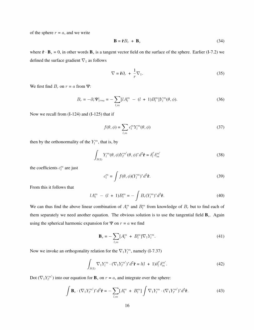
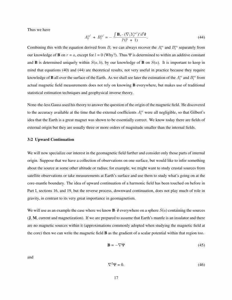
Br(r, r) =!

S(a)(a/r)2K(a/r, r · r&) Br(a, r&) d2r& (50)

where

K(x, cos)) =1

4!

1" x2

(1 + x2 " 2xcos))3/2 " 1 (51)

18

Figure 3.2.1

and this function is shown in the figure. Note that the constant term comes from the need to subtract the

influence of the monopole in the generating function for Legendre polynomials.

We can use the integral to illustrate another diminishing property of upward continued fields, not obvious

from (49). A fundamental property of integrals is that

|Br(r, r)| (!

S(a)|(a/r)2K(a/r, r · r&)| |Br(a, r&)|max d2r&. (52)

Since the term in Br under the integral is constant, and the function K is positive we can evaluate the right

side, with x = a/r:!

S(a)|(a/r)2K(a/r, r · r&)| d2r& =

! 2!

0d%

! !

0sin)d)

14!

#x2(1" x2)

(1 + x2 " 2xcos))3/2 " x2&

= x2 = (a/r)2. (53)

It is an exercise for the student to evaluate the integral! From (53) it follows that

|Br(r, r)| < |Br(a, r&)|max, r > a. (54)

In words, the magnitude of Br on a sphere of radius r > a, is always less than the maximum magnitude

on the sphere of radius a; in fact, (53) implies a stronger result, that the maximum value falls off like r"2.

Technically upward continuation is bounded linear mapping.

A consequence of (54) and of (49) is that considered as a mapping from one sphere to another larger sphere,

upward continuation is stable. This means loosely that a small error in the field on the inner sphere remains

small on the outer one.

19

This is important when we consider practical upward continuation. Suppose we have the true field on S(a)

corrupted by measurement error: Br + e; we upward continue this inaccurate field to S(r), but because

we can imagine upward continuing Br and e separately (by applying (50) to each part) we see that if the

maximum error on S(a) is less than some number , > 0, then (54) assures us the maximum error on S(r)

will also be less than ,, indeed less than ,(a/r)2.

3:3 Downward Continuation

The process of upward continuation has some practical uses, for example: predicting magnetic anomalies

measured at the sea surface from values obtained near the seafloor, or using ground-based surveys to predict

the magnetic field at satellite altitudes. But it is more common to want to project field values towards their

sources; as we have already mentioned, from the earth’s surface towards the core, or from satellite orbits

down to the crust.

The ideas of the previous section work up to a point. Certainly if (45) and (46) are valid we can use (47) and

(48), then, provided the series still converges on S(r), we can use (47) even if r < a. But (49) shows that

now the shorter wavelength components of the field are magnified relative to the longer wavelength ones.

There is no integral formula like (50) because, in its derivation, you will find the required series diverges,

and so it is impossible to interchange the sum and integral.

In fact the mapping from S(a) to S(r) when r < a is an example of an unstable process. Roughly this

means small errors in the field may grow when the field is downward continued. We saw in the upward

continuation process that simply knowing that the magnitude of the measurement error everywhere on S(a)

was less than , guaranteed the error in the upward continued field would be smaller than this. That result is

no longer true in downward continuation, and is at the heart of the instability.

We illustrate the growth of error by the following simple example. As before we have a field plus error

Br + e on S(a) and |e| ( , everywhere on the sphere. Now we downward continue to the surface S(r),

with r < a. I will assert that here e can be arbitrarily large!. How can that be? Suppose the error term has

a spherical harmonic expansion comprising the single term:

rer(a, ), %) = -Y "ll (),%)

= -Nl,lsinl)e"il% (55)

where Nl,l is a normalizing factor. Then , = |-Nl,l|. From (49) we know that on S(r) e has the single

coefficient in its SH (spherical harmonic) expansion -(a/r)l+1 and so the maximum error on S(r) is

20

|-Nl,l|(a/r)l+1 or ,(a/r)l+1. For fixed r < a we can always choose l large enough, so that the error

magnitude on S(r) is as big as we please, even though it is always exactly , on S(a).

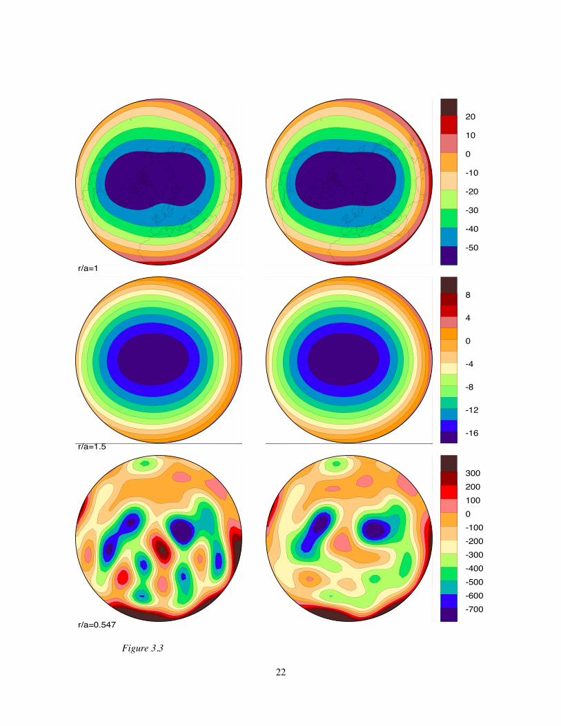
A somewhat less dry example is given pictorially on the next page, in Figure 3.3. The top two maps are

the radial field Br at the surface of the earth over the northern hemisphere, the right map from the IGRF

model for 1980, the left one deliberately disturbed by noise. The noise is not very large and it is only

just possible to see by eye the difference between the two surface maps. Below, in the second row, is the

radial field, upward continued to a radius of 1.5 earth-radii. Now the noisy and original fields are totally

indistinguishable. Notice two factors: first, the overall field size is much smaller (the units for all the maps

are µT ), conforming to the property that upward continued fields are always smaller than the originals;

second, observe how the upward continued field is almost featureless – small-scale components have been

filtered out, as predicted.

At the bottom is Br downward continued to the depth of the core. The right map (the noise-free picture)

and the left one are obviously very different – the error component has grown considerably in downward

continuation. You should notice there is still some resemblance between the two fields, but there is more

energy in the noisy map because incoherent signal has been added.

Exercise: We have shown that an error field must decrease during upward continuation, but that

is true of the field itself. Is it true that the more important quantity, the signal-to-noise ratio

always improves with upward continuation? And must this ratio always deteriorate with downward

continuation?

3:4 Geomagnetic Field Models

In our discussions of the field so far we have not dealt with the issue of how to determine the magnetic

field from a practical set of observations. In an earlier lecture it was stated that the spherical harmonic

representation provides a unique description of any magnetic field represented by a harmonic potential. The

field coefficients for rBr can, in principle be derived from equation (48):

(ml =

!

S(a)Br(a, ), %)Y m

l (),%)'d2ra2 (56)

but this evidently requires knowledge of Br all over S(a), which is not possible in practice. Before we tackle

the question of finding approximate models, and here we follow custom and say that a geomagnetic field

model is a finite collection of SH coefficients, we discuss the mathematical question of what are sufficient

measurements to define the field uniquely.

21

r/a=1

r/a=1.5

r/a=0.547

-50

-40

-30

-20

-10

0

10

20

-16

-12

-8

-4

0

4

8

-700-600-500-400-300-200-1000100200300

Figure 3.3

22

3:4.1 Geomagnetic Elements and Uniqueness

As we already noted, it is impossible to acquire complete knowledge of the radial magnetic field (or indeed

any other component) on any spherical surface. Our data are always incomplete and noisy, and consequently

there will always be ambiguity in the models derived from them. Because of this it might be argued that

the issue of uniqueness in the case of complete and perfect data is of purely academic interest. However,

experience in making magnetic field models based exclusively on one kind of observation (the magnitude

of the field) shows that this is not the case.

Equation (56) relies on knowledge of the radial magnetic field, but these are not the only kind of observations

that are made; typically when both surface survey and satellite data are involved we must consider all of the

following kinds of observations:

Br, B), B% – orthogonal components of the magnetic field in geocentric reference frame.

X , Y , Z orthogonal components of the geomagnetic field in local coordinate system,

directed north, east, and downwards respectively. This is the geodetic coordinate system.

H = (X2 + Y 2) 12 – horizontal magnetic field intensity

B = (B2) + B2

% + B2r ) 1

2 = (X2 + Y 2 + Z2) 12 – total field intensity

D = tan"1(Y/X) – declination

I = tan"1(Z/H) - inclination.

If we are prepared to accept the approximation that the Earth is a sphere, then

X = "B); Y = B%; Z = "Br. (57)

As we saw in Part I, the shape of the Earth is much better approximated by a spheroid or ellipsoid of

revolution, with equatorial radius a, polar radius b, eccentricity, e

e2 =(a2 " b2)

a2 (58)

and flattening

f =(a " b)

a= 1/298.257. (59)

Exercise:

What is the size of the error you make if you neglect to correct for the ellipsoidal shape of the earth

and use geocentric latitude and longitude in calculating the field from a spherical harmonic model?

The fact that Br on a surface S(a) uniquely determines the field (from the fact that it is the solution of a

Neumann boundary value problem for Laplace’s equation) might lead one to hope that other measurements

23

such as |B| would uniquely specify the magnetic field to within a sign. Most marine observations are of |B|

and so are many satellite measurements. Or one might anticipate that exact knowledge of the direction of

the field all over S(a) would determine the field to within a multiplicative scaling constant. Paleomagnetic

observations can determine ancient field directions much more reliably than field intensities, so one might

hope to discover the shape of the geomagnetic field in those epochs when paleomagnetic data are plentiful.

For the case of intensity data alone, George Backus showed in 1968 (Q. J. Mech and Appl. Math 21, pp

195-221, 1968; and J. Geophys. Res. 75, pp 6339-41, 1970; see also Jacobs, Geomagnetism, Vol 1, p 347)

by constructing a counter example that knowledge of |B| was not sufficient. This provided an explanation of

the poor quality of directional information predicted by models based on B alone, especially in equatorial

regions. Early satellites had only measured total field intensity, and this result led to the launching of the first

vector field satellite in 1979, known as MAGSAT. Backus’ counter example is constructed in the following

way: first find a magnetic field with potential !M that is everywhere orthogonal to a dipole field; then

!D + !M and !D "!M have the same B everywhere.

Subsequently, Khokhlov, Hulot and Le Mouel (Geophys. J. Internat. 130, pp 701-3, 1997) showed that if

knowledge of the location of the dip equator is added to knowledge of |B| everywhere then uniqueness of

the solution is guaranteed.

Similarly, (despite an earlier argument to the contrary) it was shown in 1990 by Proctor and Gubbins,

(Geophys. J. Internat. 100, pp 69-79, 1990) that B on a spherical surface does not determine the field

to within a scalar multiple. This is of some importance in the consideration of paleomagnetic data, many

of which only provide approximate geomagnetic field directions with no associated information about the

intensity. This result too has been investigated further and it has now been shown that if the magnetic field

only has two poles then knowledge of its direction everywhere allows the geomagnetic field to be recovered,

except for a constant multiplier (see Hulot, Khokhlov and Le Mouel, Geophys. J. Internat. 129, pp 347-54,

1997).

3:4.2 Construction of Field Models

We will suppose here that we have a finite collection of inaccurate observations of orthogonal components

of the geomagnetic field Bi = B · ri. Our goal is to derive from these observations the spherical harmonic

coefficients that best represent the real geomagnetic field. Clearly, we cannot use (56) because our knowledge

of Br(a, ), %) is incomplete. Also it would not make use of our measurements of the tangential part of the

field. The problem is analogous to (and in some respects identical with) that of interpolation to find a curve

24

passing through a finite number of data. Many curves will do the job, and we cannot choose which one is

more desirable without supplying additional information of some kind. One extra thing we know is that the

magnetic field obeys a differential equation, but that turns out not to be enough information by itself. When

the observations are not exact, but uncertain as in all real situations the issue is even more complicated. We

obviously shouldn’t expect the interpolant to pass through all (perhaps even any) of the observations. In the

case where we would like to downward continue a geomagnetic field model to the core-mantle boundary,

we need to be especially careful about how we deal with noise in the data; if we fit models with small scale

structure derived from this noise, then it may dominate the real signal after downward continuation.

3:4.3 Least Squares Estimation

The time-honored technique for the construction of geomagnetic field models (invented by Gauss for this

very purpose!) used to be that of least squares estimation of the spherical harmonic coefficients in a truncated

spherical harmonic expansion for the measured field components. But, instead of the exact expansion with

infinitely many terms, we decide ahead of time to model the data with an expansion truncated to degree L:

so the scalar potential is

!(r, ),%) = aL"

l=1

l"

m="l

bml

$a

r

%l + 1Y m

l (),%) (60)

and we find

B = "#!. (61)

If we measure orthogonal components of the field Br, B), B% we have a set of observations at N sites

designated rj

dj = sj · B(rj), j = 1, ..., N

=L"

l=1

l"

m="l

bml al + 2sj ·#

(Y m

l (rj)rl + 1j

)+ $j . (62)

The data dj are then linear functionals of the bml specifying the field. With an appropriate indexing scheme

for the bml we can write a prediction for our observations dj as a matrix equation.

d = Gb + n (63)

with d, n ) RN , b ) RK . G is an N !K matrix, and for each dj we can compute gkj the contribution of

the relevant spherical harmonic at that point; the vector n contains the misfits between the model predictions

and the actual measurements. The total number of parameters, the length of the vector b, is determined by

25

the truncation level: K = L(L + 2). Thus

b =

*

++,

b"11b0

1b1

1:bLL

-

../ . (64)

The value of L is chosen so that K is (much) less than N , the number of data, so there are fewer free

parameters than data to be fit. This means that it is impossible to choose b to get an exact match to the data,

and so n is not a vector of zeros. Least squares estimation involves finding the values for b that minimize

||n||2 = ||d"G · b||2, where the notation || · || is called a norm – in this case it is the ordinary length of the

vector. The idea here is to do the best job possible with the available free variables and make the model

predictions as close to the data as they can be measured by the length of the misfit vector.

Straightforward calculus can show that the LS vector can be written in terms of the solution to the normal

equations:

b = (GT G)"1GT d. (65)

Note that (65) is for several reasons not a good way to find b in a computer – first linear systems of equations

ought never to be solved by calculating a matrix inverse (it wastes time and is inaccurate); second, there is

a clever way of writing the LS equations that avoids a serious numerical precision problem arising in (65).

A result from statistics, known as the Gauss-Markov Theorem, shows that provided the misfits are due to

random, uncorrelated perturbations with zero mean, and have a common variance, then the least squares

solution is the best linear unbiased estimate (BLUE) available, in the sense that they have the smallest

variance amongst such estimates. Also

E[||n||2] = (N "K)&2 (66)

where &2 is the variance of the noise process. If the noise has a known covariance structure, then the theory

can readily be adjusted to take this into account.

A fundamental problem with this approach is that although we might have an idea of the size of the

uncertainty in the various observations, and we could choose the truncation level of the spherical harmonic

expansion so (66) is approximately satisfied, we do not know that the K spherical harmonics we have chosen

adequately describe the geomagnetic field. In other words, the misfit has two sources, not one: measurement

error and an insufficiently detailed model. To guarantee a complete description of the real field L = %; in

that case the Gauss-Markov theorem does not apply, nor does (66), and we have no uncertainty estimates

26

for our model. Truncation at finite L corresponds to an assumption about simplicity in the model that has

no physical basis – the resulting field model may be biased by the truncation procedure.

3:4.4 Regularization – an Alternative to Least Squares

An alternative to LS fitting that has been very widely used in the last decade and is the basis of almost

all modern geomagnetic field modeling is to choose “simple” models for the field of an explicit kind. To

illustrate the concept we return to our one-dimensional interpolation problem.

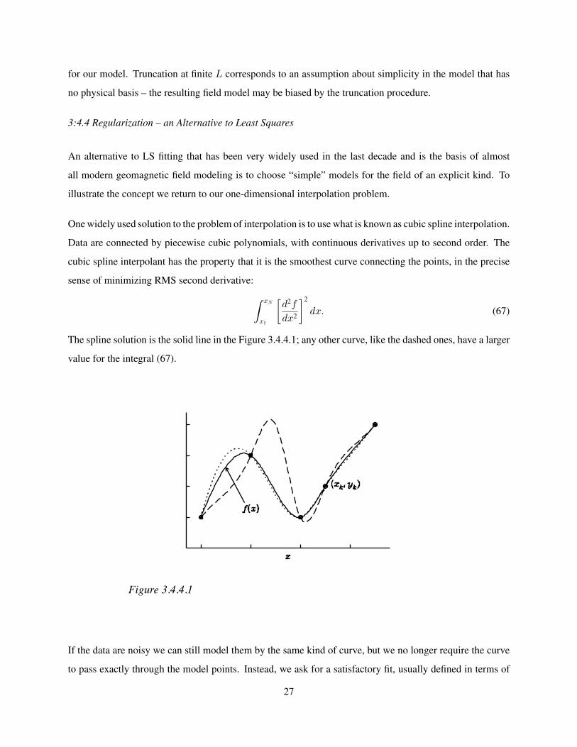
One widely used solution to the problem of interpolation is to use what is known as cubic spline interpolation.

Data are connected by piecewise cubic polynomials, with continuous derivatives up to second order. The

cubic spline interpolant has the property that it is the smoothest curve connecting the points, in the precise

sense of minimizing RMS second derivative:

! xN

x1

#d2f

dx2

&2

dx. (67)

The spline solution is the solid line in the Figure 3.4.4.1; any other curve, like the dashed ones, have a larger

value for the integral (67).

Figure 3.4.4.1

If the data are noisy we can still model them by the same kind of curve, but we no longer require the curve

to pass exactly through the model points. Instead, we ask for a satisfactory fit, usually defined in terms of

27

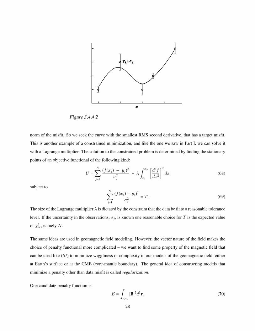
Figure 3.4.4.2

norm of the misfit. So we seek the curve with the smallest RMS second derivative, that has a target misfit.

This is another example of a constrained minimization, and like the one we saw in Part I, we can solve it

with a Lagrange multiplier. The solution to the constrained problem is determined by finding the stationary

points of an objective functional of the following kind:

U =N"

j=1

(f (xj) " yj)2

&2j

+ +

! xN

x1

#d2f

dx2

&2

dx (68)

subject toN"

j=1

(f (xj)" yj)2

&2j

= T. (69)

The size of the Lagrange multiplier + is dictated by the constraint that the data be fit to a reasonable tolerance

level. If the uncertainty in the observations, &j , is known one reasonable choice for T is the expected value

of '2N , namely N .

The same ideas are used in geomagnetic field modeling. However, the vector nature of the field makes the

choice of penalty functional more complicated – we want to find some property of the magnetic field that

can be used like (67) to minimize wiggliness or complexity in our models of the geomagnetic field, either

at Earth’s surface or at the CMB (core-mantle boundary). The general idea of constructing models that

minimize a penalty other than data misfit is called regularization.

One candidate penalty function is

E =!

r>a|B|2d3r. (70)

28

Since |B(r)|2/2µ0 is the energy density of the magnetic field at r, E/2µ0 is the total energy stored in B

outside the sphere of radius a. We can reduce this integral to a manageable form in terms of spherical

harmonics. We write B = "#!, then

E =!

r>a#! ·#! d3r. (71)

Next we make use of a familiar vector identity [number 4, in our list: # · (%A) = #% · A + %# · A, and

letting A = #!] followed by Laplace’s equation to write

E =!

[# · (!#!) " #2!] d3r

=!# · (!#!) d3r. (72)

Using Gauss’ Divergence Theorem we can rewrite the volume integral in terms of a surface integral over

S(a)

E =!

S(a)"!#!

#rd2r. (73)

Now we simply substitute the spherical harmonic expansion (60) for the potential !.

E =!

S(a)[a

"

l,m

bml Y m

l (r)]["

l&,m&

(l& + 1)bm&

l& Y m&

l& (r)]'a2d2r

= a3"

l,m

"

l&,m&

(l& + 1) bml (bm&

l& )'!

S(a)Y m

l (r)Y m&

l& (r)'d2r

= a3%"

l=1

l"

m="l

(l + 1)|bml |2. (74)

Hence E can be written as a positive weighted sum of the squared absolute values of the spherical harmonic

coefficients. This sum is now in a form we can use in minimizing an objective function like (71) for the

magnetic field. The weighting by increasing l means that higher degree (shorter wavelength) contributions

to the model will be strongly penalized in minimizing the objective functional. (74) is one example of a set

of norms (measures of size) of the kind

||B||2w =%"

l=1

wl

l"

m="l

|bml |2, wl > 0. (75)

Many interesting properties corresponding to smoothness or small size of the field can be written in this

form !

S(a)B · B d2r wl = (2l + 1)(l + 1) (76)

29

!

S(a)[#1r · B]2d2r wl = l(l + 1)2(l +

12

) (77)

!

S(a)[#2

1r · B]2d2r wl = l2(l + 1)4 (78)

!

r<aJT · JT d3r wl = a3µ2

0(l + 1)(2l + 1)2(2l + 3). (79)

In (79) JT is the toroidal part of the current flow in Earth’s core, whose significance is discussed in section

3.5. These ideas were first set out in a paper by Shure, Parker, and Backus, Phys. Earth Planet. Inter. 28,

pp 215-29, 1982.

3:4.5 Results - Gauss Coefficients

In Part I you may recall that the expansion of the Earth’s gravitational potential was called Stokes’ expansion.

In geomagnetism the honor goes to Karl Friedrich Gauss: the expansion coefficients are invariably called

Gauss coefficients. But there are some differences. First the fundamental one, that makes geomagnetism

more interesting than gravity – the field is changing on times scales of a human lifetime. So the coefficients

must always be dated. Secondly, and almost trivially, geomagnetists never use fully normalized spherical

harmonics – instead they employ an awkward real (as opposed to complex) representation in which the basis

functions (spherical harmonics) are normalized so that

!

S(1)(Y m

l )2d2r =4!

2l + 1. (80)

Then the scalar potential is written

!(r, ),%) = a%"

l=1

$a

r

%l+1 l"

m=0

Nlm(gml cosm% + hm

l sinm%)Pml (cos)) (81)

where a = 6, 371.2 km, the mean Earth radius, the Pml are the Associated Legendre functions from Part I,

andNlm = 1, m = 0

=

02(l "m)!(l + m)!

, m > 0.(82)

You will find the numbers gml , hm

l tabulated in many places. There are official models designated IGRF for

the International Geomagnetic Reference Field, agreed upon every five years by the International Association

for Geomagnetism and Aeronomy as a good approximation to the field. The linearized rate of change of

the field is also given for interpolation or extrapolation across the five year period. We are currently at

Version 10 and the model coefficients can be found at http://www.ngdc.noaa.gov/IAGA/vmod/igrf.html.

30

See Langel’s chapter in Jacob’s book Geomagnetism, an article rich in nuance, with a detailed description

of how these are computed, and many tables. Below is the IGRF-9, 2000. The values are in nanotesla.

Figure 3.4.5 shows various views of the radial component of the magnetic field from IGRF 2000: top is Br

at Earth’s surface; middle the non-dipole contribution to Br at Earth’s surface and the bottom panel gives

Br downward continued to the core-mantle boundary.

31