Embed Size (px)
Citation preview

2 – Discontinuous Galerkin Methods for Flow Problems
Per-Olof Persson
Department of Mathematics, University of California, BerkeleyMathematics Department, Lawrence Berkeley National Laboratory
Summer School on Discontinuous Galerkin MethodsInternational Center for Numerical Methods in Engineering
Barcelona, Spain
June 11-15, 2012

Outline
1 Introduction
2 The DG Method for Navier-Stokes
Application: Implicit Large Eddy Simulation
3 Curved Mesh Generation
4 Artificial Viscosity and Shock Capturing
Application: RAE2822
5 ALE for Deforming Domains
Application: Vertical Axis Wind Turbines
Application: Flapping Flight of Bat

Motivation
Need for higher fidelity predictions in computational fluid dynamicsTurbulent flows, fluid/structure interaction, flapping flightWave propagation, multiscale phenomena, non-linear interactions
Widely believed that high-order methods will become the standard
in future generations of simulation software
The DG method has emerged as one of the most promising
schemes, since it provides high-order accuracy on fully
unstructured meshes

Why Unstructured Meshes?
Complex geometries need flexible element topologies
Complex solution fields need spatially variable resolution
Fully automated mesh generators for CAD geometries are based
on unstructured simplex elements
Real-world simulation software dominated by unstructured mesh
discretization schemes

Why high-order accurate methods?
Scalar convection equation ut + ux = 0
High-order gives superior performance for equal resolution

Numerical Schemes for Flow Problems
Complex flow features→ High-order accuracy required
Complex geometries, adaptation→ Unstructured grids required
Discontinuous Galerkin (DG) methods have these properties:
FVM FDM FEM DG
1) High-order/Low dispersion
2) Unstructured meshes
3) Stability for conservation laws
However, still several problems to resolve:
High CPU/memory requirements (compared to FVM or H-O FDM)Low tolerance to under-resolved featuresHigh-order geometry representation and mesh generation

Governing Equations
The (compressible) Navier-Stokes equations:
∂ρ
∂t+
∂
∂xi(ρui) = 0,
∂
∂t(ρui) +
∂
∂xi(ρuiuj + p) = +
∂τij
∂xjfor i = 1, 2, 3,
∂
∂t(ρE) +
∂
∂xi(uj(ρE + p)) = −∂qj
∂xj+
∂
∂xj(ujτij),
with
τij = µ
(∂ui
∂xj+∂uj
∂xi− 2
3∂uk
∂xjδij
), qj = − µ
Pr∂
∂xj
(E +
pρ− 1
2ukuk
)p = (γ − 1)ρ
(E − 1
2ukuk
)When µ = 0, reduces to first-order system – Euler’s equations of
gas dynamics

Outline
1 Introduction
2 The DG Method for Navier-Stokes
Application: Implicit Large Eddy Simulation
3 Curved Mesh Generation
4 Artificial Viscosity and Shock Capturing
Application: RAE2822
5 ALE for Deforming Domains
Application: Vertical Axis Wind Turbines
Application: Flapping Flight of Bat

The Discontinuous Galerkin Method
(Reed/Hill 1973, Lesaint/Raviart 1974, Cockburn/Shu 1989-, etc)
Write the first-order equations as a system of conservation laws:
ut +∇ · Fi(u) = 0
Triangulate domain Ω into elements κ ∈ Th
Seek approximate solution uh in space of element-wise
polynomials:
Vph = v ∈ L2(Ω) : v|κ ∈ Pp(κ) ∀κ ∈ Th
Multiply by test function vh ∈ Vph and integrate over element κ:∫
κ[(uh)t +∇ · Fi(uh)] vh dx = 0

The Discontinuous Galerkin Method
Integrate by parts:∫κ
[(uh)t] vh dx−∫κ
Fi(uh)∇vh dx +
∫∂κ
Fi(u+h ,u
−h , n)v+h ds = 0
with numerical flux function Fi(uL,uR, n) for left/right states uL,uR in
direction n (Godunov, Roe, Osher, Van Leer, Lax-Friedrichs, etc)
Global problem: Find uh ∈ Vph such
that this weighted residual is zero for
all vh ∈ Vph
Error = O(hp+1) for smooth solutions∂κ
κ
n
uL
uR

The DG Method – Observations
Reduces to the finite volume method for p = 0:
(uh)tAκ +
∫∂κ
Fi(u+h ,u
−h , n) ds = 0
Boundary conditions enforced naturally for any degree p
Block-diagonal mass matrix (no overlap between basis functions)
Block-wise compact stencil – neighboring elements connected
Mass Matrix Jacobian
∂κ
κ
n
uL
uR
Viscous Discretization
Write equations as system of first order equations:
ut +∇ · Fi(u)−∇ · Fv(u,σ) = 0
σ −∇u = 0
Discretize using DG, choose appropriate numerical fluxes:
For inviscid component Fi, use approximate Riemann solvers(Godunov, Roe, Osher, Van Leer, Lax-Friedrichs, etc)For viscous component Fv, use numerical fluxes σ, u according tomethods such as IP/BR2/LDG/CDG

Implementation: The 3DG Software Package
High-order discretizations on unstructured meshes
Optimized C++ code with MATLAB and Python interfaces
Capable of simulating challenging problems:- complex real-world geometries- transitional flows, multiple scales- moving and deforming domains- fluid-structure interactions
General multiphysics framework
applicable to a wide range of
challenging problems Thin Structures
Unsteady Flows Aeroacoustics

Example: ILES at Re = 60,000
Implicit Large Eddy Simulations for flow past airfoil
Separation and transition well captured
Vortical structures: iso-surfaces of q-criterion (∇2p/2ρ)

Example: ILES at Re = 60,000
Good agreement with XFoil and previously published ILES
[Uranga/Persson/Drela/Peraire ’11]
Average pressure and skin friction coefficients

Outline
1 Introduction
2 The DG Method for Navier-Stokes
Application: Implicit Large Eddy Simulation
3 Curved Mesh Generation
4 Artificial Viscosity and Shock Capturing
Application: RAE2822
5 ALE for Deforming Domains
Application: Vertical Axis Wind Turbines
Application: Flapping Flight of Bat

Curved Mesh Generation
Automatic generation of non-inverted curved elements largely an
unresolved problem
In general this is a global problem,
affecting many elements except for
simple isotropic 2-D meshes
In [Persson/Peraire ’09], we proposed
a non-linear solid mechanics approach,
where the mesh is considered an
elastic deformable solid

Curved Mesh Generation using Solid Mechanics
The initial, straight-sided mesh corresponds to undeformed solid
External forces come from the true boundary data
Solving for a force equilibrium gives the deformed, curved,
boundary conforming mesh
Bottom-up approach can be used to obtain the boundary data
Reference domain, initial configuration Equilibrium solution, final curved mesh

Tetrahedral Mesh of Falcon Aircraft
Real-world mesh with coarse but realistic elements
Unstructured Delaunay refinement mesh, with highly curved
boundary segments
Many elements would invert with a local element-wise approach
Tetrahedral mesh Elements with I < 0.5

Outline
1 Introduction
2 The DG Method for Navier-Stokes
Application: Implicit Large Eddy Simulation
3 Curved Mesh Generation
4 Artificial Viscosity and Shock Capturing
Application: RAE2822
5 ALE for Deforming Domains
Application: Vertical Axis Wind Turbines
Application: Flapping Flight of Bat

Artificial Viscosity for Underresolved Features
Cannot resolve all solution features (shocks, RANS, singularities)
Low dissipation makes DG sensitive to underresolution
Detect by sensors and add viscosity [Persson/Peraire 06,07]
Enables shock capturing with sub-cell resolution and robust
solution of Spalart-Alamaras RANS model
Mach Sensor

Shock Sensor
Regularity of solution determined from the decay rate of
expansion coefficients in orthogonal basis
Example: Periodic Fourier case: f (x) =∑∞
k=−∞ gkeikx
If f (x) has m continuous derivatives→ |gk| ∼ k−(m+1)
For simplices: Expand solution in orthonormal Koornwinder basis:
u =
N(p)∑i=1
uiψi, u =
N(p−1)∑i=1
uiψi, se = log10
((u − u, u − u)e
(u, u)e
)Determine elemental piecewise constant εe
εe =
0 if se < s0 − κε02
(1 + sin π(se−s0)
2κ
)if s0 − κ ≤ se ≤ s0 + κ
ε0 if se > s0 + κ
.
where ε0 ∼ h/p, s0 ∼ 1/p4 and κ empirical

Example: RAE2822
Turbulent RANS flow (M = 0.675, α = 2.31o,Re = 6.5 · 106)
p-converged solution, fixed resolution h/p
p = 2 (constant h/p) p = 4
CL = 0.6144 CD = 0.0104 CL = 0.6131 CD = 0.0103

Example: RAE2822
Turbulent RANS flow (M = 0.675, α = 2.31o,Re = 6.5 · 106)
p-converged solution, fixed resolution h/p
p = 2 (constant h/p) p = 4
CL = 0.6144 CD = 0.0104 CL = 0.6131 CD = 0.0103

Example: RAE2822
Highly accurate boundary forces even with coarse meshes
Cp Cf
0 0.2 0.4 0.6 0.8 1
−1.5
−1
−0.5
0
0.5
1
x/c
Cp
p =4p =2
0 0.2 0.4 0.6 0.8 1−3
−2
−1
0
1
2
3
4
5
6
x 10−3
x/c
Cf
p =4p =2

Example: RAE2822, Transonic
Transonic flow (M = 0.729,Re = 6.5 · 106)
Sub-cell resolution of shocks
p = 4

Example: RAE2822, Transonic
Transonic flow (M = 0.729,Re = 6.5 · 106)
Sub-cell resolution of shocks
p = 4

Outline
1 Introduction
2 The DG Method for Navier-Stokes
Application: Implicit Large Eddy Simulation
3 Curved Mesh Generation
4 Artificial Viscosity and Shock Capturing
Application: RAE2822
5 ALE for Deforming Domains
Application: Vertical Axis Wind Turbines
Application: Flapping Flight of Bat

ALE Formulation for Deforming Domains
Use mapping-based ALE formulation for moving domains
[Visbal/Gaitonde ’02], [Persson/Bonet/Peraire ’09]
Map from reference domain V to physical deformable domain v(t)
Introduce the mapping deformation gradient G and the
mapping velocity vX as
G = ∇XG
vX =∂G∂t
∣∣∣∣X
and set g = det(G)
Transform equations to
account for the motion
X1
X2
NdA
V
x1
x2
nda
vG , g, vX

Transformed Equations
The system of conservation laws in the physical domain v(t)
∂Ux
∂t
∣∣∣∣x
+ ∇x · Fx(Ux,∇xUx) = 0
can be written in the reference configuration V as
∂UX
∂t
∣∣∣∣X
+ ∇X · FX(UX,∇XUX) = 0
where
UX = gUx , FX = gG−1Fx − UXG−1vX
and
∇xUx = ∇X(g−1UX)G−T = (g−1∇XUX − UX∇X(g−1))G−T
Details in [Persson/Bonet/Peraire ’09], including how to satisfy the
so-called Geometric Conservation Law (GCL)

ALE Formulation for Deforming Domains
Mapping-based formulation
gives arbitrarily high-order
accuracy in space and time
10−1
100
10−8
10−6
10−4
10−2
100
Element size h
L 2−er
ror
p=1
p=2
p=3
p=4
p=5
12
1
6
MappedUnmapped
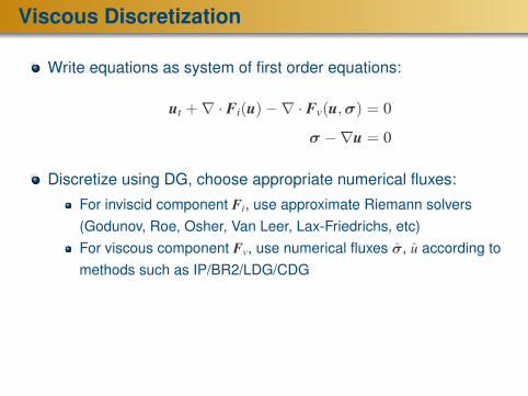
Vertical Axis Wind Turbines
Recent interest in vertical axis wind turbines (VAWT):2D airfoils, easy to manufacture, supportable at both endsOmnidirectional (good in gusty, low wind, e.g. close to ground)Lower blade speeds – lower noise and impactCan be packed close together in wind farms
Numerical simulations can help overcome remaining challenges:Lower theoretical (andpractical) efficiency thanHAWTsSensitive to design conditionsStructural problems, fatigue andcatastrophic failure
Windterra ECO 1200 1Kw VAWT

Vertical Axis Wind Turbines
Experimental design by G. Dahlbacka (LBNL) and collaborators
3kW unit, CAD design (left) and assembled unit (right)

VAWT – Mathematical Model and Discretization
Preliminary 2D simulation, using vertical symmetry
Solve the Navier-Stokes equations in a rotating frame:
G(X,Y, t) =
[cosωt − sinωt
sinωt cosωt
][X
Y
]
Hybrid boundary layer/unstructured mesh, element degree p = 3

VAWT – Numerical Results
Simulation with freestream wind speed 12 m/s (horizontally, from
the left) and wing tip speed ratio 1.5
Visualization by z-vorticity in rotating frame
0 0.1 0.2 0.3 0.4 0.5 0.6 0.7−40
−30
−20
−10
0
10
20
30
40
50
60
Moment on each blade vs. time

Bio-Inspiration for Flapping Wing MAVs
Develop high-order accurate
simulation capabilities that
capture the complex physics
in flapping flight
Use the computational tools
for increased understanding
and to design optimized
flapping kinematics

Domain Mapping
Highly complex wing motion from measured data
Construct mapping G(X, t) numerically by nonlinear solid
mechanics approach [Persson ’09]
A reference mesh (left) is deformed elastically to smoothly align
with the prescribed wing motion (right)
Grid velocity vX = ∂G∂t
∣∣X defined consistently with DIRK scheme
G(X, t)

Flapping Bat Flight Simulation
Visualization of Mach number on isosurface of entropy
Unphysical separation around simplified animal “body”

Optimal Design of Flapping Wings
Goal: Automatically generate optimized
flapping wing kinematics [Persson/Willis ’11]
A multifidelity approach, with wake-only,
panel, and high-order DG methods
Example: Flapping wing pair, prescribed
camber, solve for optimal wing twist
distribution