Embed Size (px)
Citation preview
2. Dynamic Versions of R-trees
The survey by Gaede and Guenther [69] annotates a vast list of citations re-lated to multi-dimensional access methods and, in particular, refers to R-treesto a significant extent. In this chapter, we are further focusing on the familyof R-trees by enlightening the similarities and differences, advantages and dis-advantages of the variations in a more exhaustive manner. As the number ofvariants that have appeared in the literature is large, we group them accordingto the special characteristics of the assumed environment or application, andwe examine the members of each group.
In this chapter, we present dynamic versions of the R-tree, where the ob-jects are inserted on a one-by-one basis, as opposed to the case where a specialpacking technique can be applied to insert an a priori known static set of ob-jects into the structure by optimizing the storage overhead and the retrievalperformance. The latter case will be examined in the next chapter. In simplewords, here we focus on the way dynamic insertions and splits are performedin assorted R-tree variants.
2.1 The R+-tree
The original R-tree has two important disadvantages that motivated the studyof more efficient variations:
1. The execution of a point location query in an R-tree may lead to the inves-tigation of several paths from the root to the leaf level. This characteristicmay lead to performance deterioration, specifically when the overlap ofthe MBRs is significant.
2. A few large rectangles may increase the degree of overlap significantly,leading to performance degradation during range query execution, due toempty space.
R+-trees were proposed as a structure that avoids visiting multiple pathsduring point location queries, and thus the retrieval performance could beimproved [211, 220]. Moreover, MBR overlapping of internal modes is avoided.This is achieved by using the clipping technique. In simple words, R+-trees donot allow overlapping of MBRs at the same tree level. In turn, to achieve this,inserted objects have to be divided in two or more MBRs, which means that a
15
16 2. Dynamic Versions of R-trees
specific object’s entries may be duplicated and redundantly stored in severalnodes.
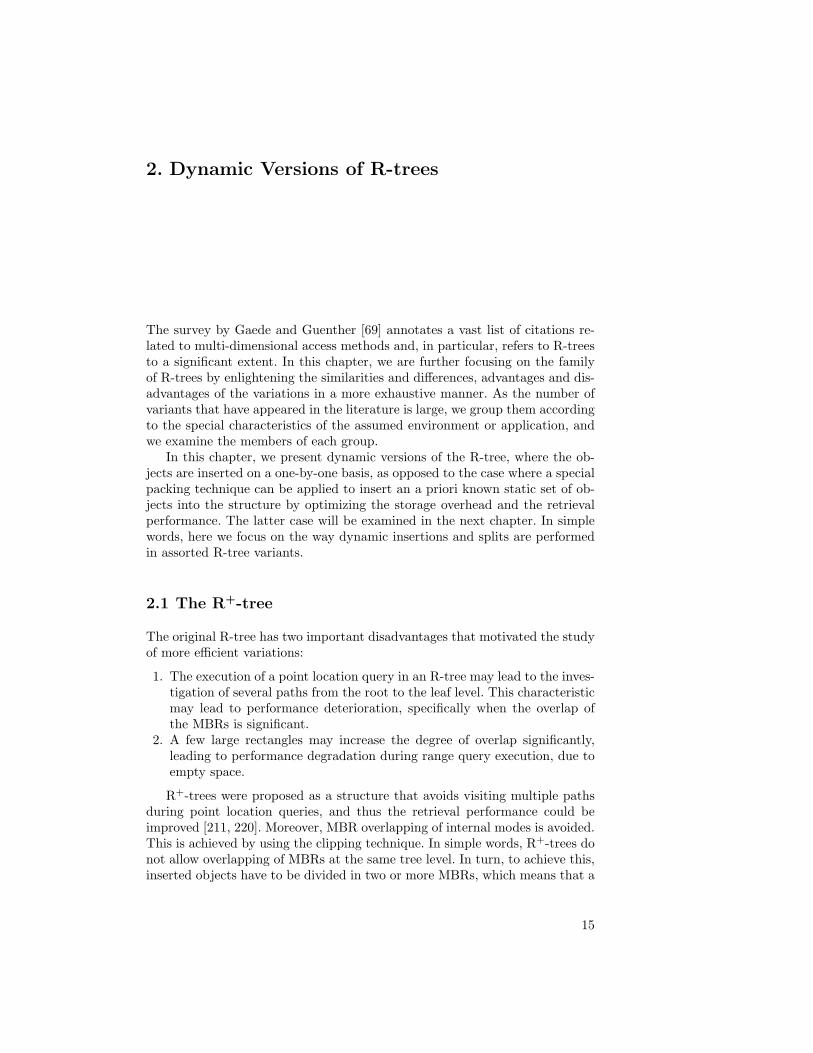
Figure 2.1 demonstrates an R+-tree example. Although the structure lookssimilar to that of the R-tree, notice that object d is stored in two leaf nodesB and C. Also, notice that due to clipping no overlap exists between nodes atthe same level.
Fig. 2.1. An R+-tree example.
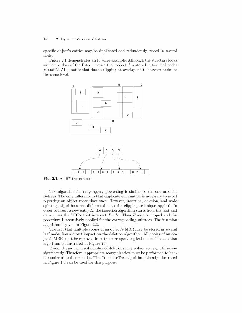
The algorithm for range query processing is similar to the one used forR-trees. The only difference is that duplicate elimination is necessary to avoidreporting an object more than once. However, insertion, deletion, and nodesplitting algorithms are different due to the clipping technique applied. Inorder to insert a new entry E, the insertion algorithm starts from the root anddetermines the MBRs that intersect E.mbr. Then E.mbr is clipped and theprocedure is recursively applied for the corresponding subtrees. The insertionalgorithm is given in Figure 2.2.
The fact that multiple copies of an object’s MBR may be stored in severalleaf nodes has a direct impact on the deletion algorithm. All copies of an ob-ject’s MBR must be removed from the corresponding leaf nodes. The deletionalgorithm is illustrated in Figure 2.3.
Evidently, an increased number of deletions may reduce storage utilizationsignificantly. Therefore, appropriate reorganization must be performed to han-dle underutilized tree nodes. The CondenseTree algorithm, already illustratedin Figure 1.8 can be used for this purpose.
2.1 The R+-tree 17
Algorithm Insert(TypeEntry E, TypeNode RN)/* Inserts a new entry E in the R+-tree rooted at node RN */
1. if RN is not a leaf node2. foreach entry e of RN3. if e.mbr overlaps with E.mbr4. Call Insert(E, e.ptr)5. endif6. endfor7. else // RN is a leaf node8. if there is available space in RN9. Add E to RN10. else11. Call SplitNode(RN)12. Perform appropriate tree reorganization to reflect changes13. endif14. endif
Fig. 2.2. The R+-tree insertion algorithm.
Algorithm Delete(TypeEntry E, TypeNode RN)/* Deletes an existing entry E from the R+-tree rooted at node RN */
1. if RN is not a leaf node2. foreach entry e of RN3. if e.mbr overlaps with E.mbr4. Call Delete (E,e.ptr)5. Calculate the new MBR of the node6. Adjust the MBR of the parent node accordingly7. endif8. endfor9. else // RN is a leaf node10. Remove E from RN .11. Adjust the MBR of the parent node accordingly12. endif
Fig. 2.3. The R+-tree deletion algorithm.
During the execution of the insertion algorithm a node may become full,and therefore no more entries can be stored in it. To handle this situation, anode splitting mechanism is required as in the R-tree case. The main differencebetween the R+-tree splitting algorithm and that of the R-tree is that down-ward propagation may be necessary, in addition to the upward propagation.Recall that in the R-tree case, upward propagation is sufficient to guaranteethe structure’s integrity.
Therefore, this redundancy works in the opposite direction of decreasingthe retrieval performance in case of window queries. At the same time, anotherside effect of clipping is that during insertions, an MBR augmentation may lead
18 2. Dynamic Versions of R-trees
to a series of update operations in a chain reaction type. Also, under certaincircumstances, the structure may lead to a deadlock, as, for example, when asplit has to take place at a node with M+1 rectangles, where every rectangleencloses a smaller one.
2.2 The R*-tree
R∗-trees [19] were proposed in 1990 but are still very well received and widelyaccepted in the literature as a prevailing performance-wise structure that isoften used as a basis for performance comparisons. As already discussed, theR-tree is based solely on the area minimization of each MBR. On the otherhand, the R∗-tree goes beyond this criterion and examines several others, whichintuitively are expected to improve the performance during query processing.The criteria considered by the R∗-tree are the following:
Minimization of the area covered by each MBR. This criterion aimsat minimizing the dead space (area covered by MBRs but not by theenclosed rectangles), to reduce the number of paths pursued during queryprocessing. This is the single criterion that is also examined by the R-tree.
Minimization of overlap between MBRs. Since the larger the overlap-ping, the larger is the expected number of paths followed for a query, thiscriterion has the same objective as the previous one.
Minimization of MBR margins (perimeters). This criterion aims atshaping more quadratic rectangles, to improve the performance of queriesthat have a large quadratic shape. Moreover, since quadratic objects arepacked more easily, the corresponding MBRs at upper levels are expectedto be smaller (i.e., area minimization is achieved indirectly).
Maximization of storage utilization. When utilization is low, more nodestend to be invoked during query processing. This holds especially for largerqueries, where a significant portion of the entries satisfies the query. More-over, the tree height increases with decreasing node utilization.
The R∗-tree follows an engineering approach to find the best possible com-binations of the aforementioned criteria. This approach is necessary, becausethe criteria can become contradictory. For instance, to keep both the areaand overlap low, the lower allowed number of entries within a node can bereduced. Therefore, storage utilization may be impacted. Also, by minimizingthe margins so as to have more quadratic shapes, the node overlapping maybe increased.
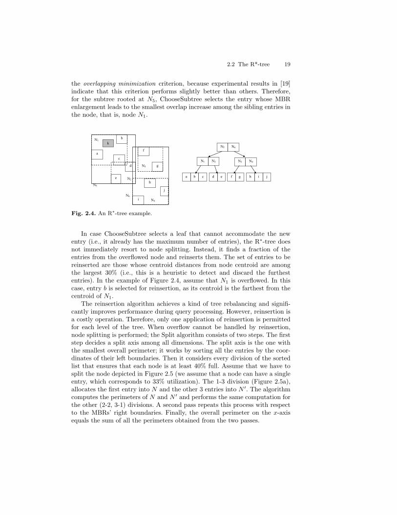
For the insertion of a new entry, we have to decide which branch to follow, ateach level of the tree. This algorithm is called ChooseSubtree. For instance, weconsider the R∗-tree depicted in Figure 2.4. If we want to insert data rectangler, ChooseSubtree commences from the root level, where it chooses the entrywhose MBR needs the least area enlargement to cover r. The required nodeis N5 (for which no enlargement is needed at all). Notice that the examinedcriterion is area minimization. For the leaf nodes, ChooseSubtree considers
2.2 The R*-tree 19
the overlapping minimization criterion, because experimental results in [19]indicate that this criterion performs slightly better than others. Therefore,for the subtree rooted at N5, ChooseSubtree selects the entry whose MBRenlargement leads to the smallest overlap increase among the sibling entries inthe node, that is, node N1.
a
k
b
c
d
e
N1
N2
f
gN3
i
j
h
N4
N5
N6
N5 N6
N1 N2 N3 N4
a b c d e f g h i j
Fig. 2.4. An R∗-tree example.
In case ChooseSubtree selects a leaf that cannot accommodate the newentry (i.e., it already has the maximum number of entries), the R∗-tree doesnot immediately resort to node splitting. Instead, it finds a fraction of theentries from the overflowed node and reinserts them. The set of entries to bereinserted are those whose centroid distances from node centroid are amongthe largest 30% (i.e., this is a heuristic to detect and discard the furthestentries). In the example of Figure 2.4, assume that N1 is overflowed. In thiscase, entry b is selected for reinsertion, as its centroid is the farthest from thecentroid of N1.
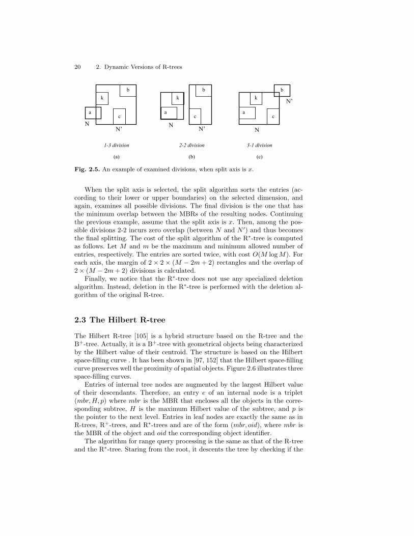
The reinsertion algorithm achieves a kind of tree rebalancing and signifi-cantly improves performance during query processing. However, reinsertion isa costly operation. Therefore, only one application of reinsertion is permittedfor each level of the tree. When overflow cannot be handled by reinsertion,node splitting is performed; the Split algorithm consists of two steps. The firststep decides a split axis among all dimensions. The split axis is the one withthe smallest overall perimeter; it works by sorting all the entries by the coor-dinates of their left boundaries. Then it considers every division of the sortedlist that ensures that each node is at least 40% full. Assume that we have tosplit the node depicted in Figure 2.5 (we assume that a node can have a singleentry, which corresponds to 33% utilization). The 1-3 division (Figure 2.5a),allocates the first entry into N and the other 3 entries into N ′. The algorithmcomputes the perimeters of N and N ′ and performs the same computation forthe other (2-2, 3-1) divisions. A second pass repeats this process with respectto the MBRs’ right boundaries. Finally, the overall perimeter on the x-axisequals the sum of all the perimeters obtained from the two passes.
20 2. Dynamic Versions of R-trees
b
k
ca
NN’
b
k
ca
NN’
b
k
ca
N
N’
1-3 division
(a)
2-2 division
(b)
3-1 division
(c)
Fig. 2.5. An example of examined divisions, when split axis is x.
When the split axis is selected, the split algorithm sorts the entries (ac-cording to their lower or upper boundaries) on the selected dimension, andagain, examines all possible divisions. The final division is the one that hasthe minimum overlap between the MBRs of the resulting nodes. Continuingthe previous example, assume that the split axis is x. Then, among the pos-sible divisions 2-2 incurs zero overlap (between N and N ′) and thus becomesthe final splitting. The cost of the split algorithm of the R∗-tree is computedas follows. Let M and m be the maximum and minimum allowed number ofentries, respectively. The entries are sorted twice, with cost O(M log M). Foreach axis, the margin of 2 × 2 × (M − 2m + 2) rectangles and the overlap of2× (M − 2m + 2) divisions is calculated.
Finally, we notice that the R∗-tree does not use any specialized deletionalgorithm. Instead, deletion in the R∗-tree is performed with the deletion al-gorithm of the original R-tree.
2.3 The Hilbert R-tree
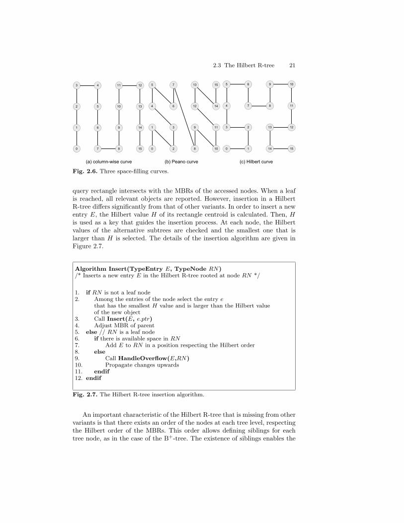
The Hilbert R-tree [105] is a hybrid structure based on the R-tree and theB+-tree. Actually, it is a B+-tree with geometrical objects being characterizedby the Hilbert value of their centroid. The structure is based on the Hilbertspace-filling curve . It has been shown in [97, 152] that the Hilbert space-fillingcurve preserves well the proximity of spatial objects. Figure 2.6 illustrates threespace-filling curves.
Entries of internal tree nodes are augmented by the largest Hilbert valueof their descendants. Therefore, an entry e of an internal node is a triplet(mbr,H, p) where mbr is the MBR that encloses all the objects in the corre-sponding subtree, H is the maximum Hilbert value of the subtree, and p isthe pointer to the next level. Entries in leaf nodes are exactly the same as inR-trees, R+-trees, and R∗-trees and are of the form (mbr, oid), where mbr isthe MBR of the object and oid the corresponding object identifier.
The algorithm for range query processing is the same as that of the R-treeand the R∗-tree. Staring from the root, it descents the tree by checking if the
2.3 The Hilbert R-tree 21
Fig. 2.6. Three space-filling curves.
query rectangle intersects with the MBRs of the accessed nodes. When a leafis reached, all relevant objects are reported. However, insertion in a HilbertR-tree differs significantly from that of other variants. In order to insert a newentry E, the Hilbert value H of its rectangle centroid is calculated. Then, His used as a key that guides the insertion process. At each node, the Hilbertvalues of the alternative subtrees are checked and the smallest one that islarger than H is selected. The details of the insertion algorithm are given inFigure 2.7.
Algorithm Insert(TypeEntry E, TypeNode RN)/* Inserts a new entry E in the Hilbert R-tree rooted at node RN */
1. if RN is not a leaf node2. Among the entries of the node select the entry e
that has the smallest H value and is larger than the Hilbert valueof the new object
3. Call Insert(E, e.ptr)4. Adjust MBR of parent5. else // RN is a leaf node6. if there is available space in RN7. Add E to RN in a position respecting the Hilbert order8. else9. Call HandleOverflow(E,RN)10. Propagate changes upwards11. endif12. endif
Fig. 2.7. The Hilbert R-tree insertion algorithm.
An important characteristic of the Hilbert R-tree that is missing from othervariants is that there exists an order of the nodes at each tree level, respectingthe Hilbert order of the MBRs. This order allows defining siblings for eachtree node, as in the case of the B+-tree. The existence of siblings enables the

22 2. Dynamic Versions of R-trees
delay of a node split when this node overflows. Instead of splitting a nodeimmediately after its capacity has been exceeded, we try to store some entriesin sibling nodes. A split takes place only if all siblings are also full. Thisunique property of the Hilbert R-tree helps considerably in storage utilizationincrease, and avoids unnecessary split operations. The decision to perform asplit is controlled by the HandleOverflow algorithm, which is illustrated inFigure 2.8. In the case of a split, a new node is returned by the algorithm.
Algorithm HandleOverflow(TypeEntry E, TypeNode RN)/* Takes care of the overflowing node RN upon insertion of E.Returns a new node NN in the case of a split, and NULL otherwise */
1. Let E denote the set of entries of node RN and its s-1 sibling nodes2. Set E = E ∪ E3. if there exists a node among the s-1 siblings that is not full4. Distribute all entries in E among the s nodes
respecting the Hilbert ordering5. Return NULL6. else // all s-1 siblings are full7. Create a new node NN8. Distribute all entries in E among the s+1 nodes9. Return the new node NN10. endif
Fig. 2.8. The Hilbert R-tree overflow handling algorithm.
A split takes place only if all s siblings are full, and thus s+1 nodes areproduced. This heuristic is similar to that applied in B∗-trees, where redistri-bution and 2-to-3 splits are performed during node overflows [111].
It is evident that the Hilbert R-tree acts like a B+-tree for insertions andlike an R-tree for queries. According to the authors’ experimentation in [105],Hilbert R-trees were proven to be the best dynamic version of R-trees as ofthe time of publication. However, this variant is vulnerable performance-wiseto large objects. Moreover, by increasing the space dimensionality, proximityis not preserved adequately by the Hilbert curve, leading to increased overlapof MBRs in internal tree nodes.
2.4 Linear Node Splitting
Ang and Tan in [11] have proposed a linear algorithm to distribute the objectsof an overflowing node in two sets. The primary criterion of this algorithm is todistribute the objects between the two nodes as evenly as possible, whereas thesecond criterion is the minimization of the overlapping between them. Finally,the third criterion is the minimization of the total coverage.
2.4 Linear Node Splitting 23
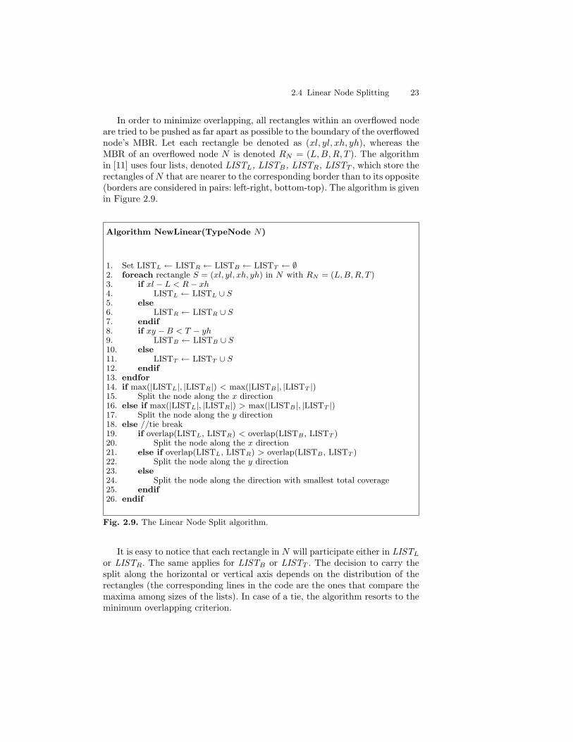
In order to minimize overlapping, all rectangles within an overflowed nodeare tried to be pushed as far apart as possible to the boundary of the overflowednode’s MBR. Let each rectangle be denoted as (xl, yl, xh, yh), whereas theMBR of an overflowed node N is denoted RN = (L,B, R, T ). The algorithmin [11] uses four lists, denoted LISTL, LISTB, LISTR, LISTT , which store therectangles of N that are nearer to the corresponding border than to its opposite(borders are considered in pairs: left-right, bottom-top). The algorithm is givenin Figure 2.9.
Algorithm NewLinear(TypeNode N)
1. Set LISTL ← LISTR ← LISTB ← LISTT ← ∅2. foreach rectangle S = (xl, yl, xh, yh) in N with RN = (L, B, R, T )3. if xl − L < R− xh4. LISTL ← LISTL ∪ S5. else6. LISTR ← LISTR ∪ S7. endif8. if xy −B < T − yh9. LISTB ← LISTB ∪ S10. else11. LISTT ← LISTT ∪ S12. endif13. endfor14. if max(|LISTL|, |LISTR|) < max(|LISTB |, |LISTT |)15. Split the node along the x direction16. else if max(|LISTL|, |LISTR|) > max(|LISTB |, |LISTT |)17. Split the node along the y direction18. else //tie break19. if overlap(LISTL, LISTR) < overlap(LISTB , LISTT )20. Split the node along the x direction21. else if overlap(LISTL, LISTR) > overlap(LISTB , LISTT )22. Split the node along the y direction23. else24. Split the node along the direction with smallest total coverage25. endif26. endif
Fig. 2.9. The Linear Node Split algorithm.
It is easy to notice that each rectangle in N will participate either in LISTL
or LISTR. The same applies for LISTB or LISTT . The decision to carry thesplit along the horizontal or vertical axis depends on the distribution of therectangles (the corresponding lines in the code are the ones that compare themaxima among sizes of the lists). In case of a tie, the algorithm resorts to theminimum overlapping criterion.
24 2. Dynamic Versions of R-trees
As mentioned in [11], the algorithm may have a disadvantage in the casethat most rectangles in node N (the one to be split) form a cluster, whereas afew others are outliers. This is because then the sizes of the lists will be highlyskewed. As a solution, Ang and Tan proposed reinsertion of outliers.
Experiments using this algorithm have shown that it results in R-trees withbetter characteristics and better performance for window queries in comparisonwith the quadratic algorithm of the original R-tree.
2.5 Optimal Node Splitting
As has been described in Section 2.1, three node splitting algorithms wereproposed by Guttman to handle a node overflow. The three algorithms havelinear, quadratic, and exponential complexity, respectively. Among them, theexponential algorithm achieves the optimal bipartitioning of the rectangles, atthe expense of increased splitting cost. On the other hand, the linear algorithmis more time efficient but fails to determine an optimal rectangle bipartition.Therefore, the best compromise between efficiency and bipartition optimalityis the quadratic algorithm.
Garcia, Lopez, and Leutenegger elaborated the optimal exponential algo-rithm of Guttman and reached a new optimal polynomial algorithm O(nd),where d is the space dimensionality and n = M +1 is the number of entries ofthe node that overflows [71]. For n rectangles the number of possible biparti-tions is exponential in n. Each bipartition is characterized by a pair of MBRs,one for each set of rectangles in each partition. The key issue, however, is thata large number of candidate bipartitions share the same pair of MBRs. Thishappens when we exchange rectangles that do not participate in the formula-tion of the MBRs. The authors show that if the cost function used dependsonly on the characteristics of the MBRs, then the number of different MBRpairs is polynomial. Therefore, the number of different bipartitions that mustbe evaluated to minimize the cost function can be determined in polynomialtime.
The proposed optimal node splitting algorithm investigates each of theO(n2) pairs of MBRs and selects the one that minimizes the cost function.Then each one of the rectangles is assigned to the MBR that it is enclosed by.Rectangles that lie at the intersection of the two MBRs are assigned to one ofthem according to a selected criterion.
In the same paper, the authors give another insertion heuristic, which iscalled sibling-shift. In particular, the objects of an overflowing node are op-timally separated in two sets. Then one set is stored in the specific node,whereas the other set is inserted in a sibling node that will depict the mini-mum increase of an objective function (e.g., expected number of disk accesses).If the latter node can accommodate the specific set, then the algorithm ter-minates. Otherwise, in a recursive manner the latter node is split. Finally, theprocess terminates when either a sibling absorbs the insertion or this is notpossible, in which case a new node is created to store the pending set. The
2.6 Branch Grafting 25
authors reported that the combined use of the optimal partitioning algorithmand the sibling-shift policy improved the index quality (i.e., node utilization)and the retrieval performance in comparison to the Hilbert R-trees, at thecost of increased insertion time. This has been demonstrated by an extensiveexperimental evaluation with real-life datasets.
2.6 Branch Grafting
More recently, in [208] an insertion heuristic was proposed to improve theshape of the R-tree so that the tree achieves a more elegant shape, with asmaller number of nodes and better storage utilization. In particular, thistechnique considers how to redistribute data among neighboring nodes, so asto reduce the total number of created nodes. The approach of branch graftingis motivated by the following observation. If, in the case of node overflow,we examined all other nodes to see if there is another node (at the samelevel) able to accommodate one of the overflowed node’s rectangles, the splitcould be prevented. Evidently, in this case, a split is performed only whenall nodes are completely full. Since the aforementioned procedure is clearlyprohibitive as it would dramatically increase the insertion cost, the branchgrafting method focuses only on the neighboring nodes to redistribute an entryfrom the overflowed node. Actually, the term grafting refers to the operationof moving a leaf or internal node (along with the corresponding subtree) fromone part of the tree to another.
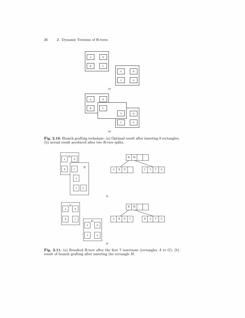
The objectives of branch grafting are to achieve better-shaped R-trees andto reduce the total number of nodes. Both these factors can improve perfor-mance during query processing. To illustrate these issues, the following ex-ample is given in [208]. Assume that we are inserting eight rectangles (withthe order given by their numbering), which are depicted in Figure 2.10. Letthe maximum (minimum) number of entries within a node be equal to 4 (2).Therefore, the required result is shown in Figure 2.10(a), because they clearlyform two separate groups. However, by using theR-tree insertion algorithm,which invokes splitting after each overflow, the result in Figure 2.10(b) wouldbe produced.
Using the branch and grafting method, the split after the insertion of rect-angle H can be avoided. Figure 2.11(a) illustrates the resulted R-tree after theinsertion of the first seven rectangles (i.e., A to G). When rectangle H has tobe inserted, the branch grafting method finds out that rectangle 3 is coveredby node R1, which has room for one extra rectangle. Therefore, rectangle Cis moved from node R2 to node R1, and rectangle H can be inserted in R2
without causing an overflow. The resulted R-tree is depicted in Figure 2.11(b).In summary, in case of node overflow, the branch grafting algorithm first
examines the parent node, to find the MBRs that overlap the MBR of theoverflowed node. Next, individual records in the overflowed are examined tosee if they can be moved to the nodes corresponding to the previously foundoverlapping MBRs. Records are moved only if the resulting area of coverage for
26 2. Dynamic Versions of R-trees
A D
B C
E H
F G
(a)
A D
B
H
F G
(b)
C
E
Fig. 2.10. Branch grafting technique: (a) Optimal result after inserting 8 rectangles;(b) actual result produced after two R-tree splits.
A D
B C
E
F G
R1 R2
A B D C E F G
A D
B C
E H
F G
(b)
R1
R2
R1
R2
R1 R2
A B D C H E F G
(a)
Fig. 2.11. (a) Resulted R-tree after the first 7 insertions (rectangles A to G); (b)result of branch grafting after inserting the rectangle H.
2.7 Compact R-trees 27
the involved nodes does not have to be increased after the moving of records.In the case that no movement is possible, a normal node split takes place.
In general, the approach of branch grafting has some similarities with theforced reinsertion, which is followed by the R∗-tree. Nevertheless, as mentionedin [208], branch grafting is not expected to outperform forced reinsertion duringquery performance. However, one may expect that, because branch graftingtries to locally handle the overflow, the overhead to the insertion time willbe smaller than that of forced reinsertion. In [208], however, the comparisonconsiders only various storage utilization parameters, not query processingperformance.
2.7 Compact R-trees
Huang et al. proposed Compact R-trees, a dynamic R-tree version with optimalspace overhead [93]. The motivation behind the proposed approach is that R-trees, R+-trees, and R∗-trees suffer from the storage utilization problem, whichis around 70% in the average case. Therefore, the authors improve the insertionmechanism of R-trees to a more compact R-tree structure, with no penalty onperformance during queries.
The heuristics applied are simple, meaning that no complex operations arerequired to significantly improve storage utilization. Among the M+1 entries ofan overflowing node during insertions, a set of M entries is selected to remainin this node, under the constraint that the resulting MBR is the minimumpossible. Then the remaining entry is inserted to a sibling that:
– has available space, and– whose MBR is enlarged as little as possible.
Thus, a split takes place only if there is no available space in any of the siblingnodes.
Performance evaluation results reported in [93] have shown that the storageutilization of the new heuristic is between 97% and 99%, which is a greatimprovement. A direct impact of the storage utilization improvement is thefact that fewer tree nodes are required to index a given dataset. Moreover,less time is required to build the tree by individual insertions, because ofthe reduced number of split operations required. Finally, caching is improvedbecause the buffer associated with the tree requires less space to accommodatetree nodes. It has been observed that the query performance of window queriesis similar to that of Guttman’s R-tree.
2.8 cR-trees
Motivated by the analogy between separating of R-tree node entries duringthe split procedure on the one hand and clustering of spatial objects on the
28 2. Dynamic Versions of R-trees
other hand, Brakatsoulas et al. [32] have altered the assumption that an R-treeoverflowing node has to necessarily be split in exactly two nodes. In particu-lar, using the k-means clustering algorithm as a working example, they imple-mented a novel splitting procedure that results in up to k nodes (k ≥ 2 beinga parameter).
In fact, R-trees and their variations (R∗-trees, etc.) have used heuristictechniques to provide an efficient splitting of M+1 entries of a node thatoverflows into two groups (minimization of area enlargement, minimization ofoverlap enlargement, combinations, etc.). On the other hand, Brakatsoulas etal. observed that node splitting is an optimization problem that takes a localdecision according to the objective that the probability of simultaneous accessto the resulting nodes after split is minimized during a query operation. In-deed, clustering maximizes the similarity of spatial objects within each cluster(intracluster similarity) and minimizes the similarity of spatial objects acrossclusters (intercluster similarity). The probability of accessing two node rect-angles during a selection operation (hence, the probability of traversing twosubtrees) is proportional to their similarity. Therefore, node splitting should(a) assign objects with high probability of simultaneous access to the samenode and (b) assign objects with low probability of simultaneous access to dif-ferent nodes. Taking this into account, the authors considered the R-tree nodesplitting procedure as a typical clustering problem of finding the “optimal” kclusters of n = M + 1 entries (k ≥ 2).
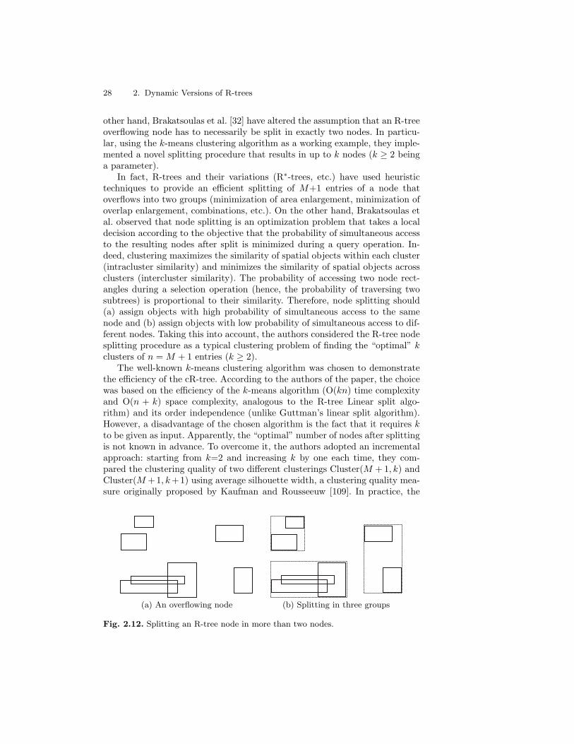
The well-known k-means clustering algorithm was chosen to demonstratethe efficiency of the cR-tree. According to the authors of the paper, the choicewas based on the efficiency of the k-means algorithm (O(kn) time complexityand O(n + k) space complexity, analogous to the R-tree Linear split algo-rithm) and its order independence (unlike Guttman’s linear split algorithm).However, a disadvantage of the chosen algorithm is the fact that it requires kto be given as input. Apparently, the “optimal” number of nodes after splittingis not known in advance. To overcome it, the authors adopted an incrementalapproach: starting from k=2 and increasing k by one each time, they com-pared the clustering quality of two different clusterings Cluster(M + 1, k) andCluster(M +1, k +1) using average silhouette width, a clustering quality mea-sure originally proposed by Kaufman and Rousseeuw [109]. In practice, the
(a) An overflowing node (b) Splitting in three groups
Fig. 2.12. Splitting an R-tree node in more than two nodes.
2.9 Deviating Variations 29
theoretical limit of kmax = M + 1 was bounded to kmax = 5 as a safe choice.An example is illustrated in Figure 2.12, where the entries of an overflowingnode are distributed in three groups.
The empirical studies provided in the paper illustrate that the cR-treequery performance was competitive with the R∗-tree and was much betterthan that of the R-tree. Considering index construction time, the cR-tree wasshown to be at the efficiency level of the R-tree and much faster than theR∗-tree.
2.9 Deviating Variations
Apart from the aforementioned R-tree variations, a number of interesting ex-tensions and adaptations have been proposed that in some sense deviate dras-tically from the original idea of R-trees. Among other efforts, we note thefollowing research works.
The Sphere-tree by Oosterom uses minimum bounding spheres instead ofMBRs [164], whereas the Cell-tree by Guenther uses minimum bounding poly-gons designed to accommodate arbitrary shape objects [77]. The Cell-tree is aclipping-based structure and, thus, a variant has been proposed to overcomethe disadvantages of clipping. The latter variant uses “oversize shelves”, i.e.,special nodes attached to internal ones, which contain objects that normallyshould cause considerable splits [78, 79].
Similarly to Cell-trees, Jagadish and Schiwietz proposed independently thestructure of Polyhedral trees or P-trees, which use minimum bounding poly-gons instead of MBRs [96, 206].
The QR-tree proposed in [146] is a hybrid access method composed of aQuadtree [203] and a forest of R-trees. The Quadtree is used to decompose thedata space into quadrants. An R-tree is associated with each quadrant, and itis used to index the objects’ MBRs that intersect the corresponding quadrant.Performance evaluation results show that for several cases the method performsbetter than the R-tree. However, large objects intersect many quadrants andtherefore the storage requirements may become high due to replication.
The S-tree by Aggarwal et al. relaxes the rule that the R-tree is a balancedstructure and may have leaves at different tree levels [5]. However, S-treesare static structures in the sense that they demand the data to be known inadvance.
A number of recent research efforts shares a common idea: to couple theR-tree with an auxiliary structure, thus sacrificing space for the performance.Ang and Tan proposed the Bitmap R-tree [12], where each node containsbitmap descriptions of the internal and external object regions except theMBRs of the objects. Thus, the extra space demand is paid off by savingsin retrieval performance due to better tree pruning. The same trade-off holdsfor the RS-tree, which is proposed by Park et al. [184] and connects an R∗-tree with a signature tree with a one-to-one node correspondence. Lastly, Lee
30 2. Dynamic Versions of R-trees
and Chung [133] developed the DR-tree, which is a main memory structurefor multi-dimensional objects. They couple the R∗-tree with this structure toimprove the spatial query performance.
Bozanis et al. have partitioned the R-tree in a number of smaller R-trees[31], along the lines of the binomial queues that are an efficient variation ofheaps.
Agarwal et al. [4] proposed the Box-tree, that is, a bounding-volume hierar-chy that uses axis-aligned boxes as bounding volumes. They provide worst-caselower bounds on query complexity, showing that Box-trees are close to opti-mal, and they present algorithms to convert Box-trees to R-trees, resulting inR-trees with (almost) optimal query complexity.
Recently, the optimization of data structures for cache effectiveness hasattracted significant attention, and methods to exploit processors’ caches havebeen proposed to reduce the latency that incurs by slow main memory speeds.Regular R-trees have large node size, which leads to poor cache performance.Kim et al. [110] proposed the CR-tree to optimize R-trees in main memoryenvironments to reduce cache misses. Nodes of main memory structures aresmall and the tree heights are usually large. In the CR-tree, MBR keys arecompressed to reduce the height of the tree. However, when transferred to adisk environment, CR-trees do not perform well. TR-trees (Two-way optimizedR-trees) have been proposed by Park and Lee [185] to optimize R-trees forboth cases, i.e., TR-trees are cache- and disk-optimized. In a TR-tree, eachdisk page maintains an R-tree-like structure. Pointers to in-page nodes arestored with fewer cost. Optimization is achieved by analytical evaluation ofthe cache latency cost of searching through the TR-tree, taking into accountthe prefetching ability of today’s CPUs.
2.9.1 PR-trees
The Priority R-tree (PR-Rtree for short) has been proposed in [15] and isa provably asymptotically optimal variation of the R-tree. The term priorityin the name of PR-tree stems from the fact that its bulk-loading algorithmutilizes the “priority rectangles”.
Before describing PR-trees, Arge et al. [15] introduce pseudo-PR-trees.In a pseudo-PR-tree, each internal node v contains the MBRs of its chil-dren nodes vc. In contrast to regular R-tree, the leaves of the pseudo-PR-tree may be stored at different levels. Also, internal nodes have de-gree equal to six (i.e., the maximum number of entries is six). More for-mally, let S be a set of N rectangles, i.e., S = r1, . . . , rN . Each ri is ofthe form (xmin(ri), ymin(ri)), (xmax(ri), ymax(ri)). Similar to Hilbert R-tree,each rectangle is mapped to a 4D point, i.e., a mapping of r∗i = (xmin(Ri),ymin(Ri), xmax(Ri), ymax(Ri)). Let S∗ be the set of N resulting 4D points. Apseudo-PR-tree TS on S is defined recursively [15]: if S contains fewer thanc rectangles (c is the maximum number of rectangles that can fit in a diskpage), then TS consists of a single leaf. Otherwise, TS consists of a node v
2.9 Deviating Variations 31
with six children, the four so-called priority leaves and two recursive pseudo-PR-trees. For the two recursive pseudo-PR-trees, v stores the correspondingMBRs. Regarding the construction of the priority leaves: the first such leafis denoted as vxmin
p and contains the c rectangles in S with minimal xmin-coordinates. Analogously, the three other leaves are defined, i.e., vymin
p , vxmaxp ,
and vymaxp . Therefore, the priority leaves store the information on the maxi-
mum/minimum of the values of coordinates. Let Sr be equal to the set thatresults from S by removing the aforementioned rectangles that correspond topriority leaves. Sr is divided into two sets S< and S> of approximately thesame size. The same definition is applied recursively for the two pseudo-PR-trees S< and S>. The division is done by using in a round-robin fashion thexmin, ymin, xmax, or ymax coordinate (a procedure that is analogous to that ofbuilding a 4D k-d-tree on S∗
r ).The following is proven in [15]: a range query on a pseudo-PR-tree on N
rectangles has I/O cost O(√
N/c + A/c), in the worst case, where A is thenumber of rectangles that satisfy the range query. Also, a pseudo-PR-tree canbe bulk-loaded with N rectangles in the plane with worst-case I/O cost equalto O(N
c logM/cNc ).
A PR-tree is a height-balanced tree, i.e., all its leaves are at the same leveland in each node c entries are stored. To derive a PR-tree from a pseudo-PR-tree, the PR-tree has to be built into stages, in a bottom-up fashion. First, theleaves V0 are created and the construction proceeds to the root node. At stage i,first the pseudo-PR-tree TSi is constructed from the rectangles Si of this level.The nodes of level i in the PR-tree consist of all the leaves of TSi , i.e., theinternal nodes are discarded. For a PR-tree indexing N rectangles, it is shownin [15] that a range query has I/O cost O(
√N/c + A/c), in the worst case,
whereas the PR-tree can be bulk-loaded with N rectangles in the plane withworst-case I/O cost equal to O(N
c logM/cNc ). For the case of d-dimensional
rectangles, it is shown that the worst-case I/O cost for the range query isO((N/c)1−1/d + A/c). Therefore, a PR-tree provides a worst-case optimality,because any other R-tree variant may require (in the worst case) the retrievalof leaves, even for queries that are not satisfied by any rectangle.
In addition to its worst-case analysis, the PR-tree has been examined ex-perimentally. In summary, the bulk-loading of a PR-tree is slower than thebulk-loading of a packed 4D Hilbert tree. However, regarding query perfor-mance, for nicely distributed real data, PR-trees perform similar to existingR-tree variants. In contrast, with extreme data (very skewed data, which con-tain rectangles with high differences in aspect ratios), PR-trees outperform allother variants, due to their guaranteed worst-case performance.
2.9.2 LR-trees
The LR-tree [31] is an index structure based on the logarithmic dynamizationmethod. LR-trees are based on decomposability. A searching problem is calleddecomposable if one can partition the input set into a set of disjoint subsets,perform the query on each subset independently, and then easily compose
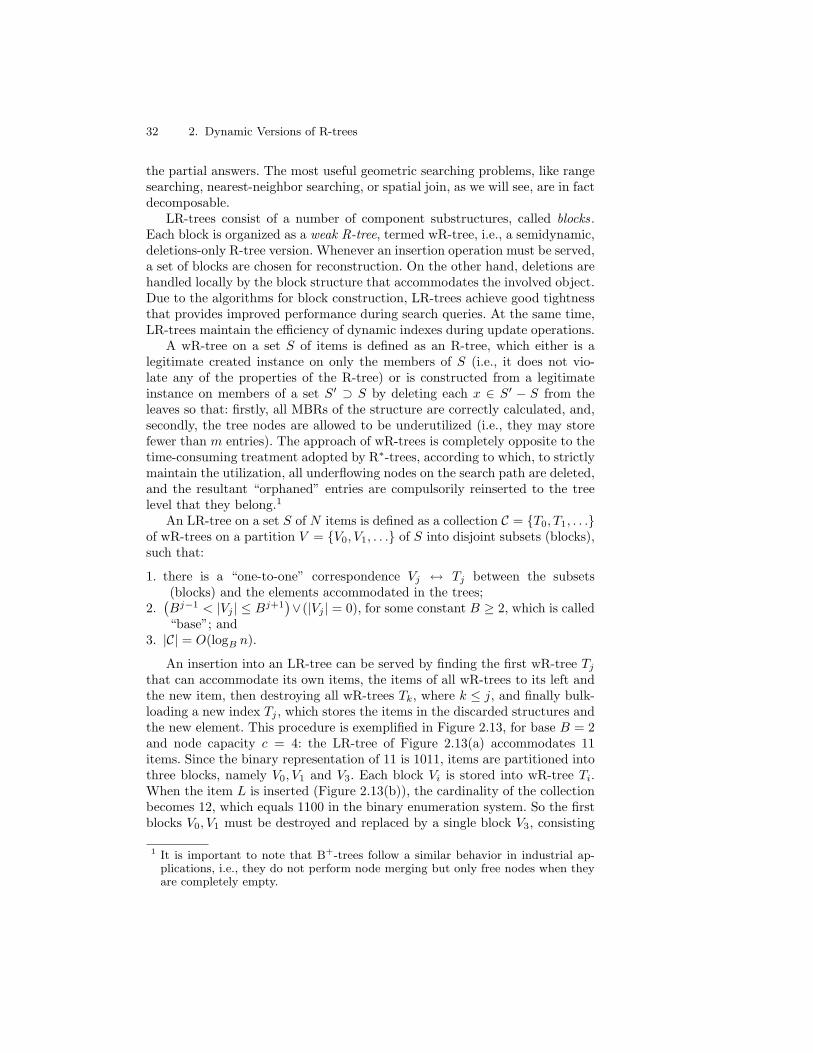
32 2. Dynamic Versions of R-trees
the partial answers. The most useful geometric searching problems, like rangesearching, nearest-neighbor searching, or spatial join, as we will see, are in factdecomposable.
LR-trees consist of a number of component substructures, called blocks.Each block is organized as a weak R-tree, termed wR-tree, i.e., a semidynamic,deletions-only R-tree version. Whenever an insertion operation must be served,a set of blocks are chosen for reconstruction. On the other hand, deletions arehandled locally by the block structure that accommodates the involved object.Due to the algorithms for block construction, LR-trees achieve good tightnessthat provides improved performance during search queries. At the same time,LR-trees maintain the efficiency of dynamic indexes during update operations.
A wR-tree on a set S of items is defined as an R-tree, which either is alegitimate created instance on only the members of S (i.e., it does not vio-late any of the properties of the R-tree) or is constructed from a legitimateinstance on members of a set S′ ⊃ S by deleting each x ∈ S′ − S from theleaves so that: firstly, all MBRs of the structure are correctly calculated, and,secondly, the tree nodes are allowed to be underutilized (i.e., they may storefewer than m entries). The approach of wR-trees is completely opposite to thetime-consuming treatment adopted by R∗-trees, according to which, to strictlymaintain the utilization, all underflowing nodes on the search path are deleted,and the resultant “orphaned” entries are compulsorily reinserted to the treelevel that they belong.1
An LR-tree on a set S of N items is defined as a collection C = {T0, T1, . . .}of wR-trees on a partition V = {V0, V1, . . .} of S into disjoint subsets (blocks),such that:
1. there is a “one-to-one” correspondence Vj ↔ Tj between the subsets(blocks) and the elements accommodated in the trees;
2.(Bj−1 < |Vj | ≤ Bj+1
)∨(|Vj | = 0), for some constant B ≥ 2, which is called
“base”; and3. |C| = O(logB n).
An insertion into an LR-tree can be served by finding the first wR-tree Tj
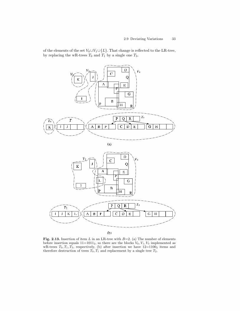
that can accommodate its own items, the items of all wR-trees to its left andthe new item, then destroying all wR-trees Tk, where k ≤ j, and finally bulk-loading a new index Tj , which stores the items in the discarded structures andthe new element. This procedure is exemplified in Figure 2.13, for base B = 2and node capacity c = 4: the LR-tree of Figure 2.13(a) accommodates 11items. Since the binary representation of 11 is 1011, items are partitioned intothree blocks, namely V0, V1 and V3. Each block Vi is stored into wR-tree Ti.When the item L is inserted (Figure 2.13(b)), the cardinality of the collectionbecomes 12, which equals 1100 in the binary enumeration system. So the firstblocks V0, V1 must be destroyed and replaced by a single block V3, consisting
1 It is important to note that B+-trees follow a similar behavior in industrial ap-plications, i.e., they do not perform node merging but only free nodes when theyare completely empty.
2.9 Deviating Variations 33
of the elements of the set V0∪V1∪{L}. That change is reflected to the LR-tree,by replacing the wR-trees T0 and T1 by a single one T3.
Fig. 2.13. Insertion of item L in an LR-tree with B=2. (a) The number of elementsbefore insertion equals 11=10112, so there are the blocks V0, V1, V3 implemented aswR-trees T0, T1, T3, respectively, (b) after insertion we have 12=11002 items andtherefore destruction of trees T0, T1 and replacement by a single tree T2.
34 2. Dynamic Versions of R-trees
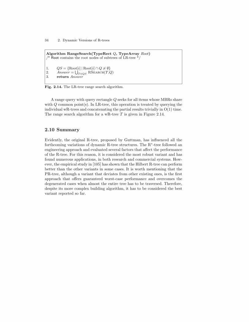
Algorithm RangeSearch(TypeRect Q, TypeArray Root)/* Root contains the root nodes of subtrees of LR-tree */
1. QS = {Root[i] | Root[i] ∩Q &= ∅}2. Answer =
⋃T∈QS RSearch(T ,Q)
3. return Answer
Fig. 2.14. The LR-tree range search algorithm.
A range query with query rectangle Q seeks for all items whose MBRs sharewith Q common point(s). In LR-tree, this operation is treated by querying theindividual wR-trees and concatenating the partial results trivially in O(1) time.The range search algorithm for a wR-tree T is given in Figure 2.14.
2.10 Summary
Evidently, the original R-tree, proposed by Guttman, has influenced all theforthcoming variations of dynamic R-tree structures. The R∗-tree followed anengineering approach and evaluated several factors that affect the performanceof the R-tree. For this reason, it is considered the most robust variant and hasfound numerous applications, in both research and commercial systems. How-ever, the empirical study in [105] has shown that the Hilbert R-tree can performbetter than the other variants in some cases. It is worth mentioning that thePR-tree, although a variant that deviates from other existing ones, is the firstapproach that offers guaranteed worst-case performance and overcomes thedegenerated cases when almost the entire tree has to be traversed. Therefore,despite its more complex building algorithm, it has to be considered the bestvariant reported so far.


![Dependent nonparametric trees for dynamic hierarchical ... · evolving trees in the literature. There exist a variety of distributions over stationary trees [1, 14, 5, 13, 10], and](https://img.pdfslide.net/doc/110x75/5fd13e4f158a3b5ebf5869bd/dependent-nonparametric-trees-for-dynamic-hierarchical-evolving-trees-in-the.jpg)


![FunSeqSet: Towards a Purely Functional Data Structure for ......Dynamic Trees Problem • We refer to the term “dynamic trees problem” to the one defined by [Sleator and Tarjan,1983]:](https://img.pdfslide.net/doc/110x75/5fa1a7435bc8a5406c4342d3/funseqset-towards-a-purely-functional-data-structure-for-dynamic-trees.jpg)