Embed Size (px)
Citation preview
Theory of the
Four Point Dynamic
Bending testPart II: Influences of
1. Overhanging Beam Ends& 2. Extra Moving Masses

Theory of theFour Point Dynamic Bending test
Part II: Influences of1.Overhanging Beam Ends
& 2. Extra Moving Masses
DWW-2002-083
Author: A.C. PronkDate: August 2002
2
Abstract
This report deals with the influences of a) the extra moving masses and b) the overhanging beam ends on the measured deflections in the dynamic four point bending test.
The analytical solution is deduced for both cases. In the case of overhanging beam-ends the exact analytical solution can be obtained directly. However, if extra moving masses (point loads) are involved the numerical value for the analytical solution has to be obtained by an iteration procedure. In the included Excel files this value is obtained after nine iterations starting with the values obtained for the case with only overhanging beam-ends. Only when the chosen frequency is near the Eigen frequencies of the system more iteration will be necessarily.
After obtaining the correct values for the deflection and the phase lag at an arbitrarily position on the beam the modified first order approximation is applied for the backcalculation of the input values for the stiffness modulus and (material) phase lag. In this way an impression is obtained for the mistakes made in the backcalculation procedures.
Next to the chapters dealing with the theory a chapter “Guidelines” is given for the use of the included zipped Excel files.
Contents- Introduction and Background p. 4- Theory p. 5- The case =0 p. 8 - Simplified Iteration Procedure if =0 p. 10- General Iteration Procedure for 0 p. 11- Backcalculation procedure p. 13- Short Guidelines for the EXCEL files Visco1 and Visco2 p. 15
- Special option in Visco1.xls for backcalculation p. 19- Remarks p. 19
DisclaimerThis working paper is issued to give those interested an opportunity to acquaint themselves with progress in this particular field of research. It must be stressed that the opinions expressed in this working paper do not necessarily reflect the official point of view or the policy of the director-general of the Rijkswaterstaat. The information given in this working paper should therefore be treated with caution in case the conclusions are revised in the course of further research or in some other way. The Kingdom of the Netherlands takes no responsibility for any losses incurred as a result of using the information contained in this working paper.
3

The influence of extra moving masses and overhanging beam endsin the Four Point Bending Test
Introduction and Background
The basic theory of the four point bending test (4PB) is well described in part I of this series (Theory of the Four Point Dynamic bending test; P-DWW-96-008; ISBN-90-3693-712-4) and will not be repeated. Thus for a good understanding of the formulas it is advised to use part I next to part II. For a good description of the 4PB test is referred to: Description of fatigue test method Four Point Bending (4PB) in use at the Dutch Road & Hydraulic Engineering Division (DWW) & Technical University Delft & Dutch Consultancy Agencies; DWW-2002-082; July 2002. Photos of an old and a new clamping device are given below in figure 1 and 2.
Figure 1. The “old” bending device.
4
Figure 2. The new four point bending deviceIn the four point bending test the applied force will not only be used for bending the beam but also for the movements of parts of the hydraulic jack and of the inner clamps and if present the sensor which is placed on the beam for measuring the deflection. In the equations the influence of the mass of the sensor can be replaced by an arbitrarily mass at the position Xsensor. Thus the losses due to the movement of the masses have to be taken into account in the data processing. In the following equations the time function has been omitted.
Theory
First of all we will use the following notations for the orthogonal polynomials used in the solution procedure (see P-DWW-96-008):
[1]
[2]
With L* = Total length of the beam; A = distance between inner and outer clamp and = distance between beginning of beam (x=0) and the first outer clamp. The distance A+ is also called Xclamp
The total deflection Vtot{x}= has to satisfy the differential equation including the boundary conditions at the beginning of the beam (moment=0) and at the outer clamp (deflection=0). The deflection is build up out of the sum of three types of deflections.
The first type Va {x} will satisfy the differential equation including the external force Fo and the forces due to extra moving masses (particular solution). It is assumed that this deflection can be written as an infinite summation of the polynomials Tn{x} with n being an odd integer number. This is correct if only the external force and the force due to an extra moving mass at the inner clamps are present, because these forces can also be developed in the polynomials Tn{x}. However, a mass force on a different position (e.g. a sensor in the middle of the beam) hampers in away such a simple solution procedure. In principle another deflection Va {x} has to be added to satisfy this mass force. This later deflection (in case of a mass at location Xsensor) is build up out of the polynomials Tn
*{x}. Nevertheless, by rewriting the mass term it is possible to handle the problem with only the first deflection Va {x} type.
[3]
The mass forces (point load) at the inner clamp and at the position of the sensor are given by:
[4]
The deflection Va {x} is represented by: [5]
The individual amplitude of each term at position x is given by:
5

By using the polynomials this deflection already satisfies the boundary condition at the beginning of the beam (x = 0 ; moment = 0). If equals zero (outer clamp at position x=0) the boundary condition for the deflection (=0 at x=) is also fulfilled. Furthermore, note that the phase lag n
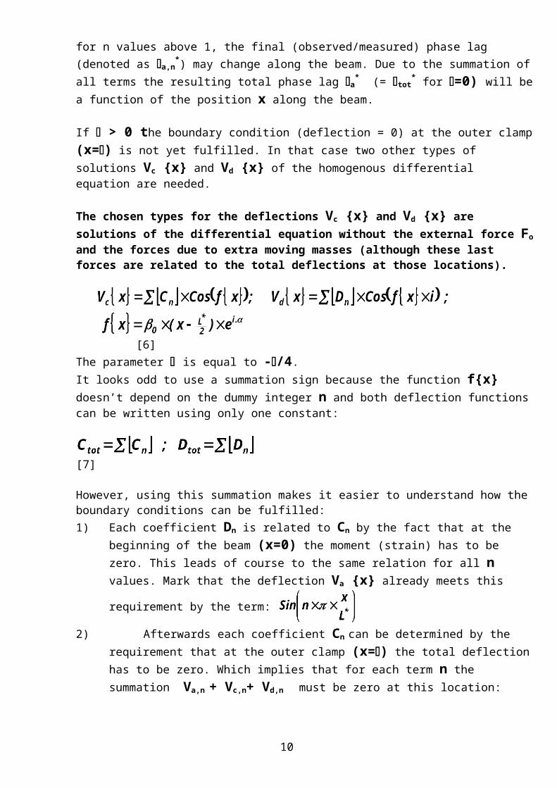
* for each separate deflection term doesn’t depend on the position x along the beam; but because the polynomial Tn {x} can change of sign along the beam for n values above 1, the final (observed/measured) phase lag (denoted as a,n
*) may change along the beam. Due to the summation of all terms the resulting total phase lag a
* (= tot* for =0) will be a function of the position x
along the beam.
If > 0 the boundary condition (deflection = 0) at the outer clamp (x=) is not yet fulfilled. In that case two other types of solutions Vc {x} and Vd {x} of the homogenous differential equation are needed.
The chosen types for the deflections Vc {x} and Vd {x} are solutions of the differential equation without the external force Fo and the forces due to extra moving masses (although these last forces are related to the total deflections at those locations).
[6]
The parameter is equal to -/4.It looks odd to use a summation sign because the function f{x} doesn’t depend on the dummy integer n and both deflection functions can be written using only one constant:
[7]
However, using this summation makes it easier to understand how the boundary conditions can be fulfilled:1) Each coefficient Dn is related to Cn by the fact that at the beginning of the beam (x=0) the
moment (strain) has to be zero. This leads of course to the same relation for all n values.
Mark that the deflection Va {x} already meets this requirement by the term:
2) Afterwards each coefficient Cn can be determined by the requirement that at the outer clamp (x=) the total deflection has to be zero. Which implies that for each term n the summation
Va,n + Vc,n+ Vd,n must be zero at this location:
[8]
For solving the differential equation the external force F0 at the two inner clamps has to be transformed into a force distribution along the beam:
[9]
Using the same procedure for the extra mass forces at the two (moving) inner clamps (x=A+) and at the position of the deflection sensor (x=xsensor) will lead to:
[10]
6

[11]
The deflection term Va must satisfy the differential equation with regard to the load conditions.
[12]
The deflection Va can also be written as a summation of the polynomials Tn{x}. It follows the deflection Va has to satisfy the next equation:
[13]
With: [14]
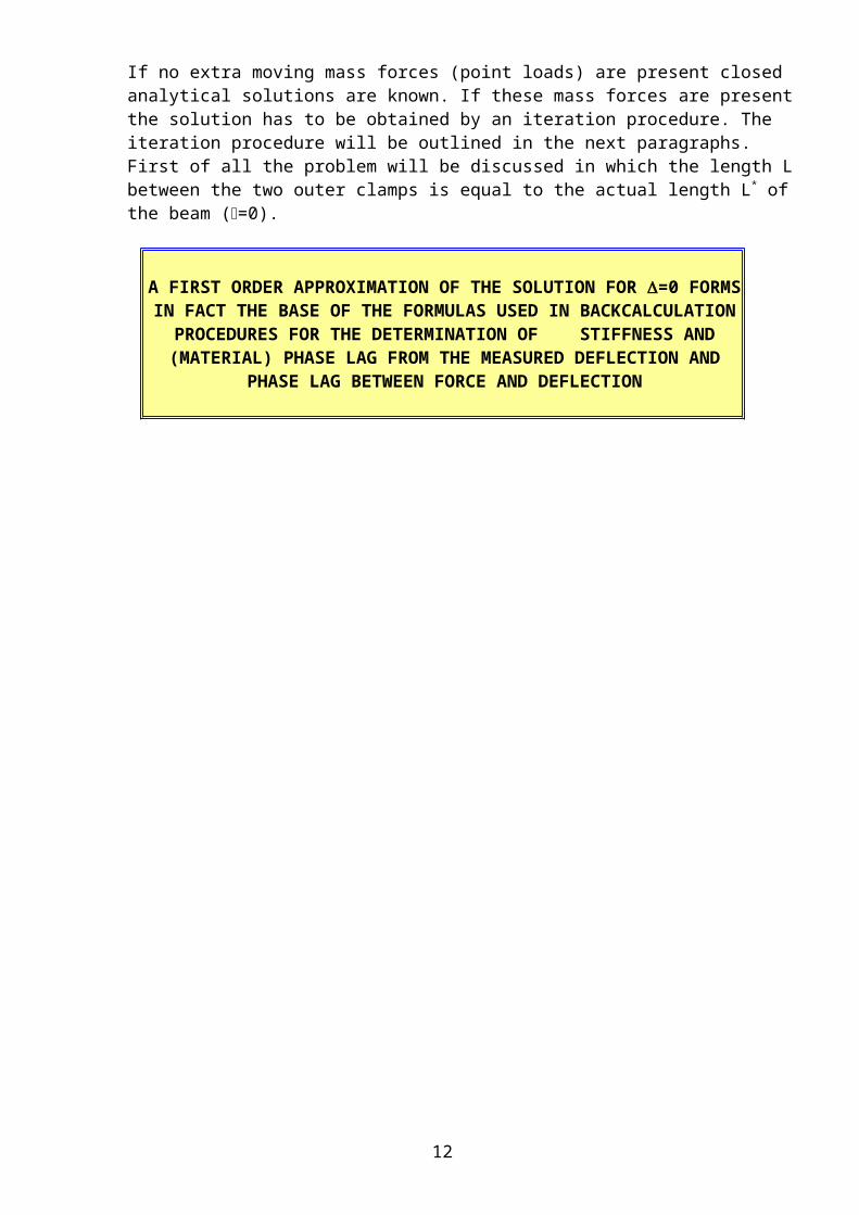
If no extra moving mass forces (point loads) are present closed analytical solutions are known. If these mass forces are present the solution has to be obtained by an iteration procedure. The iteration procedure will be outlined in the next paragraphs.First of all the problem will be discussed in which the length L between the two outer clamps is equal to the actual length L* of the beam (=0).
A FIRST ORDER APPROXIMATION OF THE SOLUTION FOR =0 FORMS IN FACT THE BASE OF THE FORMULAS USED IN
BACKCALCULATION PROCEDURES FOR THE DETERMINATION OF STIFFNESS AND (MATERIAL) PHASE LAG FROM THE MEASURED
DEFLECTION AND PHASE LAG BETWEEN FORCE AND DEFLECTION
7

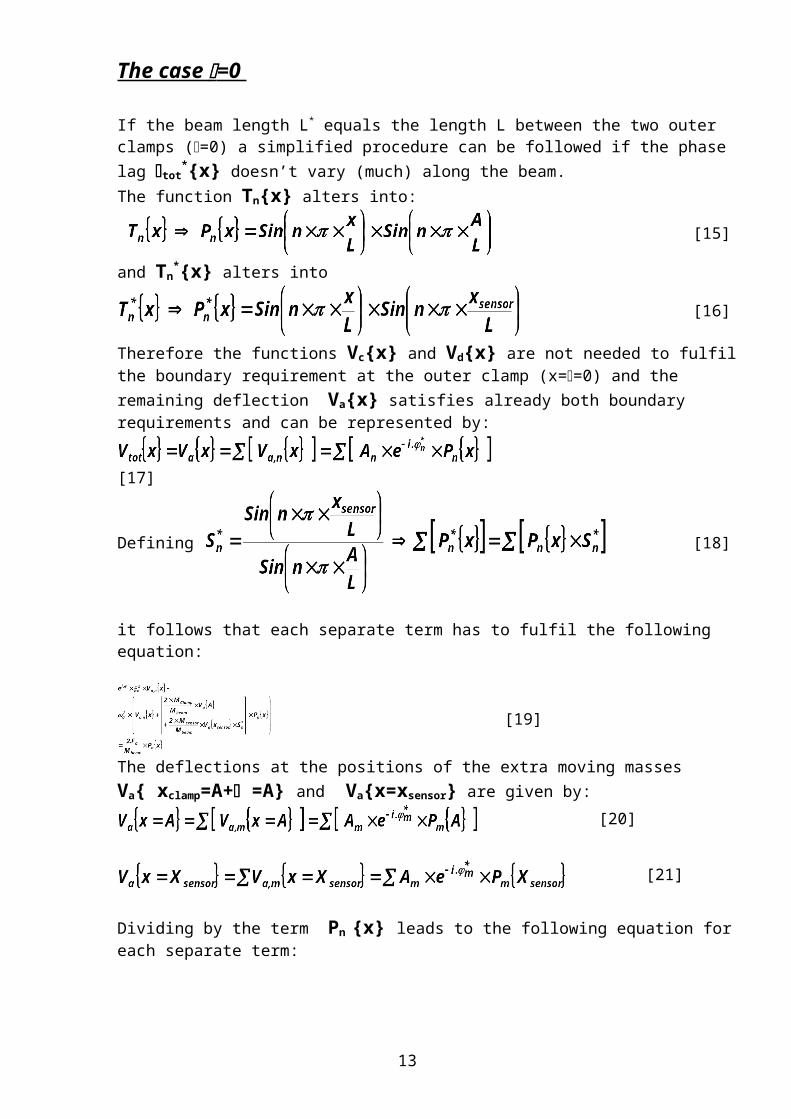
The case =0
If the beam length L* equals the length L between the two outer clamps (=0) a simplified procedure can be followed if the phase lag tot
*{x} doesn’t vary (much) along the beam.The function Tn{x} alters into:
[15]
and Tn*{x} alters into
[16]
Therefore the functions Vc{x} and Vd{x} are not needed to fulfil the boundary requirement at the outer clamp (x==0) and the remaining deflection Va{x} satisfies already both boundary requirements and can be represented by:
[17]
Defining [18]
it follows that each separate term has to fulfil the following equation:
[19]
The deflections at the positions of the extra moving masses Va{ xclamp=A+ =A} and Va{x=xsensor} are given by:
[20]
[21]
Dividing by the term Pn {x} leads to the following equation for each separate term:
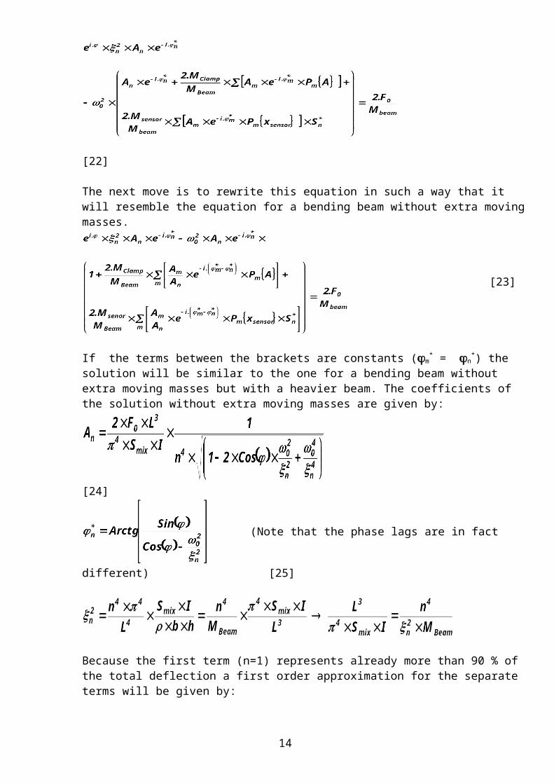
[22]
The next move is to rewrite this equation in such a way that it will resemble the equation for a bending beam without extra moving masses.
[23]
8

If the terms between the brackets are constants (m* = n
*) the solution will be similar to the one for a bending beam without extra moving masses but with a heavier beam. The coefficients of the solution without extra moving masses are given by:
[24]
(Note that the phase lags are in fact different) [25]
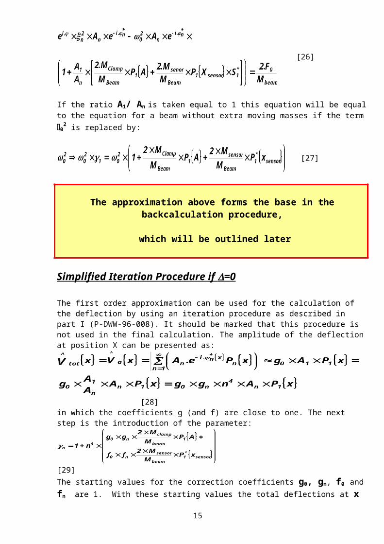
Because the first term (n=1) represents already more than 90 % of the total deflection a first order approximation for the separate terms will be given by:
[26]
If the ratio A1/ An is taken equal to 1 this equation will be equal to the equation for a beam without extra moving masses if the term 0
2 is replaced by:
[27]
The approximation above forms the base in the backcalculation procedure,
which will be outlined later
Simplified Iteration Procedure if =0
The first order approximation can be used for the calculation of the deflection by using an iteration procedure as described in part I (P-DWW-96-008). It should be marked that this procedure is not used in the final calculation. The amplitude of the deflection at position X can be presented as:
[28]in which the coefficients g (and f) are close to one. The next step is the introduction of the parameter:
9
[29]
The starting values for the correction coefficients g0, gn, f0 and fn are 1. With these starting values the total deflections at x = xclamp and x = xsensor are calculated using equations 17, 24 and 25 and the transformation for the radial frequency given by equation 27. The ratios of the total deflections at x = xclamp and x = xsensor and the first terms are used for a better approximation of g0 and f0. The coefficients g and f ought to be nearly the same.
[30]
[31]
The second steps are the calculations of ‘all’ the coefficients
The same procedure is repeated for the deflections at x = xsensor . The new values for An can be taken as a weighed mean value. The third step is the calculation of a better approximation for gn and fn. [32]
Of course g1 and f1 will be equal to 1. These three steps are repeated until the coefficients and the deflections do not change anymore.
The obtained figures for gn , fn and An can now be used for the calculation of the deflection along the whole beam.
General Iteration Procedure for 0
For the general differential equation ( > 0 and one or more extra moving masses) the following procedure can be used. First the deflection equation for each individual term is divided by the polynomial Tn{x} leading to the following equation:
[40]
Rearrangement of this equation leads to: using former (old) values for for the terms between the brackets gives:
[41]
with and [42]
and
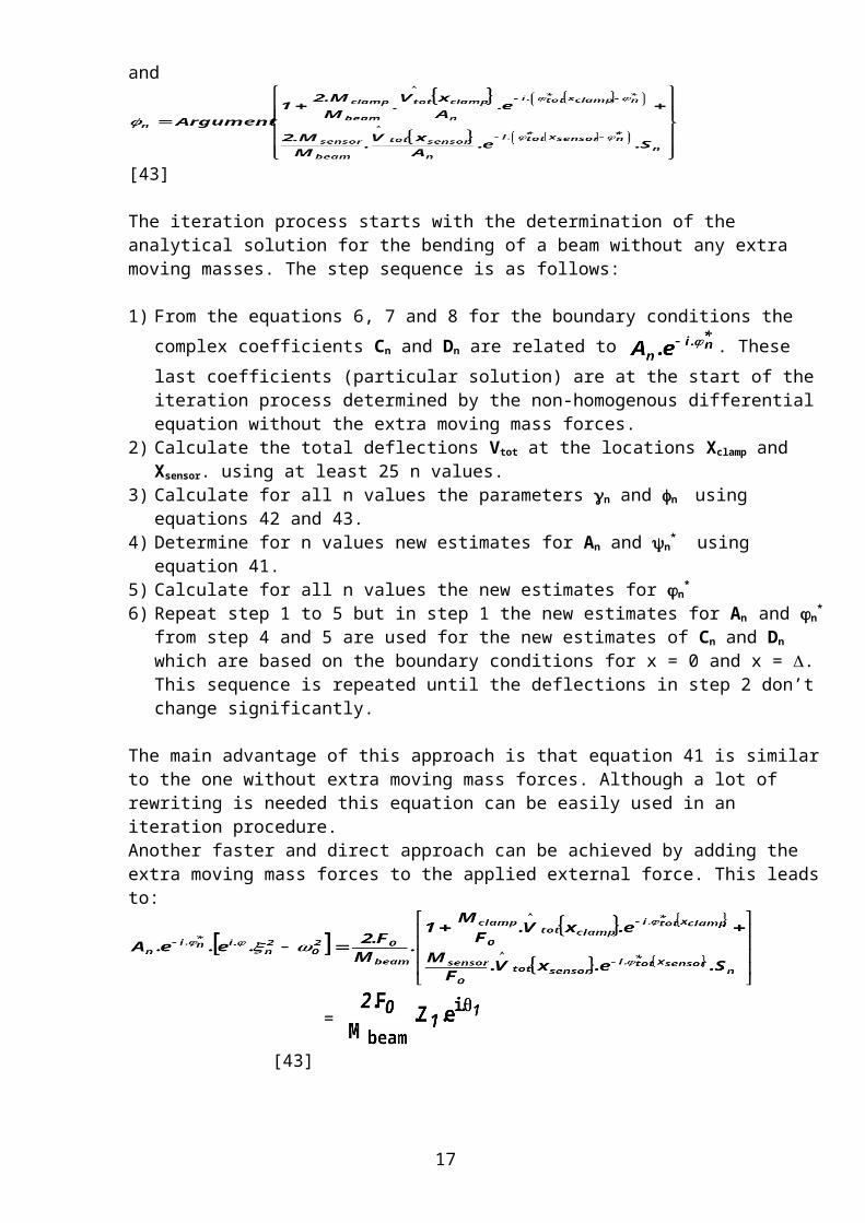
[43]
The iteration process starts with the determination of the analytical solution for the bending of a beam without any extra moving masses. The step sequence is as follows:
1) From the equations 6, 7 and 8 for the boundary conditions the complex coefficients Cn and Dn are related to . These last coefficients (particular solution) are at the start of the
10

iteration process determined by the non-homogenous differential equation without the extra moving mass forces.
2) Calculate the total deflections Vtot at the locations Xclamp and Xsensor. using at least 25 n values.3) Calculate for all n values the parameters n and n using equations 42 and 43.4) Determine for n values new estimates for An and n
* using equation 41.5) Calculate for all n values the new estimates for n
* 6) Repeat step 1 to 5 but in step 1 the new estimates for An and n
* from step 4 and 5 are used for the new estimates of Cn and Dn which are based on the boundary conditions for x = 0 and x = .This sequence is repeated until the deflections in step 2 don’t change significantly.
The main advantage of this approach is that equation 41 is similar to the one without extra moving mass forces. Although a lot of rewriting is needed this equation can be easily used in an iteration procedure. Another faster and direct approach can be achieved by adding the extra moving mass forces to the applied external force. This leads to:
= [43]
Rewriting as leads to the very simple iteration equation:
[44]
Both iteration procedures work fine. However, if the applied frequency is close to a resonance frequency the first procedure seems to be more stable.
11
Backcalculation procedure
First of all two new definitions R{x} and R’{x} are introduced:
[33]
[34]
In fact R{x} is the coefficient used in the first term of the infinite sum which represents the analytical solution for a beam with = 0. R’{x} is the mirror coefficient used in the solution of the static bending beam test.
The first order approximation for the deflection along the beam is given by:
[35]
with [36]
The deflection equation above is equal to the equation belonging to a viscous-elastic mass-spring
system with a spring constant and an equivalent mass Mequi.{x}:
[37]
Notice that both the spring constant and the equivalent mass depend on the position X at which the deflection is measured. Normally this will be at the location of the sensor, which in return is often placed in the centre of the beam (giving the highest amplitude). In that case the equivalent mass is given by equation 38.
[38]
Some equipments use the deflection measured at the inner clamp. In those cases the equivalent mass is given by:
12
[39]
Instead of the function R{x} it is better to use the modified function R’{x} which gives better results in the backcalculation. Moreover, because for decreasing frequencies the equations become equal to the ones of a quasi-static system (0 = 0).
For the equipment at the Road & Hydraulic Eng. Div. of Rijkswaterstaat the following figures are valid: Effective length L of the beam = 400 mm, Distance A between inner and outer clamp = 135 mm. With these figures the following coefficients are obtained.
Using the deflection measured at the centre of the beam:Mequivalent = 0.5731 . Mbeam + 0.8725 . Mclamp + 1.1461 . Msensor (using R{x})Mequivalent = 0.5738 . Mbeam + 0.8755 . Mclamp + 1.1423 . Msensor (using R’{x})
Using the deflection measured at the inner clamp of the beam:Mequivalent = 0.6568 . Mbeam + 1.0000 . Mclamp + 1.3136 . Mcentre (using R{x})Mequivalent = 0.6555 . Mbeam + 1.0000 . Mclamp + 1.3047 . Mcentre (using R’{x})
In case of ASTM specifications (A=L/3) the following figures are obtained:
Using the deflection measured at the centre of the beam:Mequivalent = 0.5774 . Mbeam + 0.8660 . Mclamp + 1.1547 . Msensor (using R{x})Mequivalent = 0.5785 . Mbeam + 0.8696 . Mclamp + 1.1500 . Msensor (using R’{x})
Using the deflection measured at the inner clamp of the beam:Mequivalent = 0.6667 . Mbeam + 1.0000 . Mclamp + 1.3333 . Mcentre (using R{x})Mequivalent = 0.6652 . Mbeam + 1.0000 . Mclamp + 1.3225 . Mcentre (using R’{x})
13
Short Guidelines for the EXCEL files Visco1 and Visco2
Both Excel files consist out of three tabs: “Input-Output”; “Overhanging-Beam” and “Extra-Moving-Masses”. The calculation procedures in both files are identical and differ only by the iteration procedure as described in the chapter “General Iteration Procedure for 0”.In the file Visco1.xls an extra option is given for the backcalculation if real measured deflections and phase lags are given (see below). The main tab is “Input-Output”. The process starts with the input (bold red figures) for the:
Parameter Cell Dimension Parameter Cell DimensionTotal length of
beam B2 [m] Outer spanDistance A E2 [m]
Effective length of beam (span) B3 [m] Position X of
calculation E3 [m]
Height of beam B4 [m] Position sensor E5 [m]Width of beam B5 [m] The following parameters are related to the input
and printed in blue italic characters:
- Density of the beam (B12);- The bending Moment (B13);- Overhanging Beam-end D (E4);- Position outer clamp (E6);- Position inner clamp (E7).
Mass of plunger B6 [kg]Mass of sensor B7 [kg]Mass of beam B8 [kg]
Stiffness Modulus B10 [Pa]
Material phase lag B11 [o]
Force B14 [N]
With this input the static deflection can be calculated and is given in cell E18. The value for the frequency is put into cell C19. The calculated deflection and phase lag for position X (cell E3) are given in row 19 together with the backcalculated values for Smix, phase lag and strain using the calculated deflection and phase lag in combination with the modified first order approximation. An example is given on the next page in figure 3. It should be noticed that the exact analytical solution is build up out of an infinite series of sinusoidal terms. Because the accuracy of Excel calculations is limited to around 10-24 the summation is limited also because the values of higher terms decrease fast. Furthermore, the implication of this limitation is that a value of less than 10-20 can be considered to be zero.
In cell C19 the chosen frequency [Hz] is put in. The final output is given in the same row.
On tab “Overhanging-Beam” the calculations are given if only the mass of the beam was taken into account and not the extra moving masses due to plunger and sensor. The output figures are printed in the cells of block A5 to H8 (Figure 4.). In the cells of block I5 to J9 the output for the control calculations is given with respect to boundary requirements.
At last on tab “Extra-Moving-Masses” the calculations are performed if also the extra point loads at the position of the inner clamps are taken into account. As explained before the answers have to be obtained by iteration. An example is given in figure 5. The iteration procedure starts with the values obtained from the calculations on tab “Overhanging-Beam” when only the mass of the total beam is taken into account. In total nine iterations are performed. If the chosen frequency is not close to the Eigen frequency this number of iterations is more than satisfactorily. An approximation of the first Eigen frequency is given in the cells F4 and I4 on the tab “Input-Output”.
14
ColumnsA B C D E
Beam Characteristics Positions
Total length L* [m] 0.450 Distance A (inner and outer clamp) [m] 0.135 Effective length L [m] 0.400 Xbeam [m] (X=0 :: begin of beam) 0.225 Height H [m] 0.0503 Delta 0.025 Width W [m] 0.0628 X Sensor [m] Default: = L*/2 0.225 Mass plunger Mv [kg] 5.562 Position outer clamp [m] 0.025
Mass sensor [kg] 0.140 Position inner clamp [m] = Position plunger mass 0.160
Mass beam [kg] 3.254
Material parameters Modulus Smix [Pa] 2.71E+09
Phase lag [o] 35.2 Figure 3. Input figures for tab “Input-Output” Density [kg/m3] 2289
Moment I [m4] 6.660E-07 Force F [N] 52
o 16Row 18/19 0
Static Deflection [m] 3.271E-05 Smix [Pa]
Backcalculated[o] Back
[o] Measured
[m/m] Calculated
[m/m] Actual
Ratio Ratio
SmixRatio
Frequency
[Hz] 8"Dynamic"
Deflection [m] 3.302E-05 2.713E+09 35.255 35.623 4.896E-05 4.897E-05 100.0% 100.0% 100.0%
15

Position : Xbeam Xclamp Xsensor Position : Xbeam Xclamp Xsensor CONTROL
Deflection[m] 3.280E-05 2.872E-05 3.280E-05 Smix back
[Pa] 2.713E+09 2.713E+09 2.713E+09Deflection & Strain at X=Delta
Deflection should be zero Deflection - Strain
[o] 35.35 35.35 35.35 back
[o] 35.25 35.25 35.25 2.69E-22 3.01E-07
Strain[m/m] 4.862E-05 4.841E-05 4.862E-05 Strain Cal.
[m/m] 4.863E-05 4.863E-05 4.863E-05Deflection & Strain at X=0
Strain should be zero Deflection - Strain
If only the mass of the beam is taken into account the results above are obtained 6.41E-06 1.64E-23
Figure 4Example of output figures for tab “Overhanging-Beam”
including the control calculations for the boundary requirements
Deflection and Phase at Xbeam if all masses are taken into account
16
Only Mass beam First iteration Second Third Fourth Fifth Sixth Seventh Eight Nine (It9-It8)/It9
[%]Deflection [um] 32.8 33.0 33.0 33.0 33.0 33.0 33.0 33.0 33.0 33.0 Xbeam 0.000%Phase lag [o] 35.35 35.62 35.62 35.62 35.62 35.62 35.62 35.62 35.62 35.62 Xbeam 0.000%
Control after 9 iterat. Deflection [m] 3.302E-05 28.91 28.91 28.91 28.91 28.91 28.91 28.91 28.91 Xclamp 0.000%
Deflection at X= meas. [o] 35.62 35.62 35.62 35.62 35.62 35.62 35.62 35.62 35.62 Xclamp 0.000%7.40E-21 back [o] 35.25 Xclamp Xsensor 33.02 33.02 33.02 33.02 Xsensor 0.000%
Strain at X=0 Smix back [Pa] 2.713E+09Deflection
[m] 2.891E-05 3.302E-05 35.62 35.62 35.62 35.62 Xsensor 0.000%
9.57E-22 Actual Strain [m/m] 4.897E-05
measured
[o] 35.62 35.62 Calc. Strain
[m/m] 4.896E-05 back.
[o] 35.25 35.25
DEFLECTION for Xbeam
Smix back. [Pa] 2.713E+09 2.713E+09
Figure 5.Example of output figures for tab
‘Extra-Moving-MassesActual Strain [m/m] 4.866E-05 4.897E-05
Calc. Strain [m/m]
4.896E-05 4.896E-05
17

Special option in Visco1.xls for backcalculation
A special option in Visco1.xls allows the determination of the mistake made with the modified first order backcalculation procedure and the calculation of the ‘correct’ values. This is done in block A22 till D30 of tab Input-Output. The measured deflection and phase lag are put into cells B22 and B24. Seed values for the Smix and material phase lag are put into cells B10 and B11. The program calculates the deflection and phase lag, which are related to these input values (B23 and B25). Now in cell B26 the squared sum of the deviations between measured and calculated values is determined. Using the option Solver in Excel and varying the input values for Smix and phase lag can minimize this sum. The backcalculated Smix and phase lag values are given in the cells B28 and B30. In cells C28 and C30 the deviation percentage is given.
Deflection measured real 3.2975E-05Deflection calculated 3.3018E-05
measured real 35.623
calculated 35.6232Squared Summation 1.714E-06 This value is minimized by the solver optionSmix input 2.71E+09
Minimalization by variation in input data for Smix and
Smix back 2.71E+09 -0.03%
input 35.244
backcalculated 35.255 0.03%
Figure 6. Example of the output for the special option in Visco1.xls
Remarks
1. In the Excel program file the phase angles are calculated as the argument of a complex number instead of using the arc tan function. This is done because the argument calculation gives the correct value between – and + while the arc tan function gives a value between – /2 and + /2. If the real part is denoted by a and the imaginary part by b the arc tan function only takes into account the sign of the quotient a/b while the argument function takes into account both the sign of a and the sign of b. The argument function is given by:
C.ARGUMENT(COMPLEX(a;b))2. The absolute value of a complex figure z is calculated as:
C.ABS(z) or C.ABS(COMPLEX(a;b)) or as (a2+b2)
3. The accuracy of the calculations in Excel is good but not extremely high. E.g. the constant pi is only given in 14 decimals. Therefore results smaller than 10–15 can be considered to be zero.
4. The two (free) Excel files can be ordered by sending an E-mail to:
18

5. An example is given below for a beam of 5 kg with a total length of 450 mm while the mass of the plunger is 10 kg and values for the stiffness modulus and the phase lag are 5 GPa and 20 o respectively.
Figure 7. An example of the errors made in the backcalculation using the modified first order approximation
19