Embed Size (px)
Citation preview
1
Long-term environmental monitoring for assessment of change: measurement inconsistencies 1
over time and potential solutions 2
3
Kari E. Ellingsen1*, Nigel G. Yoccoz1,2, Torkild Tveraa1, Judi E. Hewitt3, Simon F. Thrush4 4
5
1 Norwegian Institute for Nature Research (NINA), Fram Centre, P.O. Box 6606 Langnes, 9296 6
Tromsø, Norway 7
8
2 Department of Arctic and Marine Biology, UiT The Arctic University of Norway, 9037 Tromsø, 9
Norway 10
11
3 National Institute of Water and Atmospheric Research, Hamilton, New Zealand 12
13
4 Institute of Marine Sciences, University of Auckland, Auckland, New Zealand 14
15
* Corresponding author: E-mail: [email protected], Phone: +47 41223760, ORCID: 0000-16
0002-2321-8278 17
18
Acknowledgments: KEE was supported by the Norwegian Oil and Gas Association (project no. 20-19
2013), the Norwegian Environment Agency (project no. 1204110 and 4013045), the Norwegian 20
Research Council (project no. 212135) and Norwegian Institute for Nature Research (NINA). NGY 21
and TT were supported by NINA. We thank one anonymous referee for useful comments on this 22
article. 23
24
25

2
Abstract 26
27
The importance of long-term environmental monitoring and research for detecting and understanding 28
changes in ecosystems and human impacts on natural systems is widely acknowledged. Over the last 29
decades a number of critical components for successful long-term monitoring have been identified. 30
One basic component is quality assurance/quality control protocols to ensure consistency and 31
comparability of data. In Norway, the authorities require environmental monitoring of the impacts of 32
the offshore petroleum industry on the Norwegian continental shelf, and in 1996 a large-scale regional 33
environmental monitoring program was established. As a case study, we used a sub-set of data from 34
this monitoring to explore concepts regarding best practices for long-term environmental monitoring. 35
Specifically, we examined data from physical and chemical sediment samples and benthic macro-36
invertebrate assemblages from 11 stations from six sampling occasions during the period 1996-2011. 37
Despite the established quality assessment and quality control protocols for this monitoring program, 38
we identified several data challenges, such as, missing values and outliers, discrepancies in variable 39
and station names, changes in procedures without calibration, and different taxonomic resolution. 40
Furthermore, we show that the use of different laboratories over time makes it difficult to draw 41
conclusions with regard to some of the observed changes. We offer recommendations to facilitate 42
comparison of data over time. We also present a new procedure to handle different taxonomic 43
resolution so valuable historical data is not discarded. These topics have a broader relevance and 44
application than for our case study. 45
46
Keywords: data comparability; long-term monitoring; macrobenthos; oil and gas industry; taxonomic 47
resolution 48
49
3
Introduction 50
51
There is a widespread recognition of the importance of long-term environmental monitoring and 52
research for evaluating ecological responses to disturbance, and documenting and providing baselines 53
against which change or extremes can be evaluated (Lindenmayer and Likens 2010). However, there 54
are many challenges to be addressed in order to successfully assess changes and their causes 55
(Lindenmayer and Likens 2010; Hughes 2014; Lindenmayer et al. 2015). During the last decades, 56
characteristics of effective ecological monitoring have been summarized, and so have the reasons why 57
monitoring may fail (Yoccoz et al. 2001; Lindenmayer and Likens 2010; Lindenmayer et al. 2015). 58
Different designs fit different purposes, and it is important to address the question of “why monitor?” 59
and clearly specify the objectives of a proposed monitoring programme. It is also important to evaluate 60
what type, magnitude and causes of effect can or need to be detected with different designs. While it is 61
crucial that environmental monitoring of human impacts on natural systems can detect temporal 62
changes with sufficient reliability and sensitivity, estimating unbiasedly environmental changes and 63
the impact of drivers is challenging (Yoccoz et al. 2001; Desaules 2012). These are challenges that call 64
for targeted monitoring programmes designed to address specific questions (Nichols and Williams 65
2006). 66
67
Data comparability is a key requirement for any long-term monitoring program (Cao and Hawkins 68
2011). Using soil monitoring as an example, Desaules (2012) stated that measurement instability 69
occurred along the whole measurement chain, from sampling to the expression of results. National 70
monitoring programs in the US, member states of the European Union (EU) and the states of 71
Australia, among others, are facing the challenge of comparability (Hughes and Peck 2008; Buss et al. 72
2015). With regard to the implementation of two large-extent US surveys, Hughes and Peck (2008) 73
stated that consistent methods and levels of effort at all sampling points are necessary to distinguish 74
differences in status/trend in ecological condition from differences in protocol. 75
76
4
The petroleum activity on the Norwegian continental shelf started in the late 1960’s in the south, i.e. 77
the Ekofisk fields (Gray et al. 1990), and since then exploration and extraction have been moving 78
gradually northwards. Environmental monitoring in the Norwegian sector began already in 1973 at 79
Ekofisk, and a thorough analysis of the Ekofisk and Eldfisk fields was done by Gray et al. (1990). A 80
more comprehensive analysis of fields along the shelf was later done by Olsgard and Gray (1995). In 81
1996, a large-scale regional offshore environmental monitoring program, hereafter called the Regional 82
Monitoring, was established for the Norwegian continental shelf (Gray et al. 1999; Bakke et al. 2011; 83
2013), as required by the Norwegian authorities (Iversen et al. 2015). At the same time, the focus on 84
quality assurance/quality control protocols increased. In total, the Regional Monitoring covers about 85
1000 stations on the Norwegian continental shelf (Norwegian Oil and Gas 2013). The Regional 86
Monitoring covers all oil fields on the Norwegian continental shelf, and the purpose of the monitoring 87
is to provide an overview of the environmental status and trends in relation to the petroleum activities. 88
The shelf has been divided into regions, from Region I in the south (North Sea) to Region XI in the 89
north (Barents Sea, see Iversen et al. 2015), although the history and level of petroleum activity varies 90
a lot among the regions. The requirement from the authorities is that the monitoring should be 91
repeated every third year in regions with petroleum activity. In addition to all the field specific stations 92
and reference stations, a minimum of 10 so-called regional stations were established in each region 93
with petroleum activity. Some of these regional stations are in fact reference stations for specific 94
fields, whereas other regional stations are not linked to any fields. The intention was that the regional 95
stations should not be impacted by the oil and gas industry. The purpose of the establishment of these 96
regional stations was to provide data for long-term changes within a given region such as those due to 97
climate change (Gray et al. 1999). Indeed, a critical evaluation of the environmental status at such 98
regional stations can be crucial to understand human impacts vs natural variation in this marine system 99
over space and time. 100
101
The availability of adequate and sustained funding is one of the critical elements for maintaining 102
effective monitoring programs (Hewitt and Thrush 2007; Lindenmayer and Likens 2010; 103
Mieszkowska et al. 2014). Financial constraints often result in a trade-off between sampling in space 104
5
or time (Hewitt and Thrush 2007). Indeed, financial costs can have a major impact on deciding an 105
acceptable level of uncertainty and can be the limiting factor in choosing an analytical strategy 106
(Bennett et al. 2014). The Regional Monitoring is an example of a long-term monitoring program 107
where reliable funding has been secured because the oil and gas industry has a financial commitment. 108
109
Each year the Norwegian Oil and Gas Association has contracted out projects to consulting companies 110
to conduct the Regional Monitoring in some selected regions (Iversen et al. 2015). This procedure is 111
based on current Norwegian legislation. The consequence is that different companies have conducted 112
sampling, data processing, laboratory analyses, and written the survey reports for different years. 113
Although the Norwegian Environment Agency has provided guidelines for fieldwork and data 114
processing procedures and reporting (Iversen et al. 2011; 2015), this process requires successful inter-115
laboratory comparisons in practice. If this is not the situation, this procedure is in contrast to the 116
current international recommendations of data integrity, specifically linked to the critical component 117
of stability and competence of staff for long-term monitoring (e.g., Lindenmayer and Likens 2010). 118
119
According to the guidelines for the Regional Monitoring, the results should be comparable over time 120
and among different regions (Iversen et al. 2015). Data from 11 regional stations on the southern part 121
of the Norwegian continental shelf (Region I, i.e. the Ekofisk region) have given us the opportunity to 122
examine temporal (and spatial) patterns of benthic communities and environmental variables from six 123
sampling occasions over a rather extensive area, and explore best practices for long-term 124
environmental monitoring. We have identified a number of challenges with regard to measurement 125
inconsistencies over time, including outliers and missing values, discrepancies in variable and stations 126
names, changes in procedures without calibration, and different taxonomic resolution. Accordingly, 127
the Regional Monitoring is facing challenges in terms of data comparability (see e.g. Hughes and Peck 128
2008; Buss et al. 2015). Here we provide recommendations linked to the specific challenges identified 129
to facilitate comparison of data over time. Although we have only focused on a case study using 130
regional stations from one particular region, this issue is also relevant for the field specific stations in 131
this region, the other regions along the Norwegian continental shelf, and with regard to a comparison 132

6
of data among the different regions on the shelf. Clearly, these topics also have a broader relevance 133
and application than for the Norwegian Regional Monitoring. 134
135
The Regional Monitoring Protocol 136
137
The Norwegian continental shelf has been divided into 11 regions (Iversen et al. 2015). Within each 138
region, a sampling design is arranged with a set of field stations located at different distances (250 m, 139
500 m, 1000 m, 2000 m etc.) and in different directions (depending of the dominating direction of 140
currents) from each oil field, and with accompanying reference stations. In addition, the set of regional 141
stations are evenly spatially distributed within a given region (see Fig. 1 for Region I). The regional 142
stations are sampled during the same monitoring surveys as for the field stations and reference 143
stations. Over time there has been some changes in the number (and location) of regional stations 144
within regions. One reason for this may be that new oil or gas fields are established on the shelf, and 145
some regional stations are located too close to the new fields and they may now be regarded as 146
impacted by the petroleum industry. Another reason may be that fields are closed, and if a regional 147
station is the same as a reference station linked to a field, the monitoring at this station may end. 148
149
The guidelines for the Regional Monitoring, including quality assurance/quality control protocols, are 150
regularly updated (Iversen et al. 2011; 2015). These guidelines have improved, and this may 151
potentially have improved the data quality over time. Consulting companies conducting the fieldwork 152
and data processing write reports that are evaluated by the Norwegian Environment Agency and an 153
independent expert group, appointed by the agency, and finally the reports are approved by the 154
Environment Agency (Iversen et al. 2015). The data are collected in the Environmental Monitoring 155
Database (hereafter called the MOD-database), owned by the Norwegian Oil and Gas Association. 156
Although the survey reports are evaluated, the actual datasets that are included in the MOD-database 157
are not evaluated by any independent expert group. The Norwegian Environment Agency has an open 158
data policy and all data are open to public scrutiny (Olsgard and Gray 1995), which also makes the 159
data potentially available to the scientific community. The amount of data collected in the MOD-160

7
database may be considered as large at an international scale, for example, data from Regions I-IV and 161
VI-VII have been collected every third year, starting in 1996, 1997 or 1998 depending on the region. 162
163
In the Regional Monitoring, biological, physical and chemical samples are taken from the bottom 164
sediments with a 0.1 m2 van Veen grab. At each station, five replicates for analyses of macrobenthos 165
are taken. Biological samples are sieved on a 1 mm round-hole diameter sieve, and retained fauna are 166
fixed in formalin for later identification. Three additional grabs are taken at each station for analyses 167
of sediment variables. Sub-samples are taken from the upper 5 cm of the sediment for analyses of 168
physical sediment characteristics, and from the upper 1 cm for chemical analyses. Sample station 169
positioning employs a differential GPS (global positioning system, accuracy of <10 m) with the vessel 170
held in position with a dynamic positioning system (DP). 171
172
At the time when the Regional Monitoring was established, sectorial based monitoring was commonly 173
employed. However, during the last decades there has been a gradual change towards a more 174
ecosystem-based monitoring. Marine biodiversity faces unprecedented threats from multiple pressures 175
arising from human activities operating at global, regional and local scales (e.g., Mieszkowska et al. 176
2014; Thrush et al. 2015). On the Norwegian continental shelf, for example, the oil and gas industry is 177
unlikely to be the only driver of change in a changing world and in a multi-use ecosystem. With regard 178
to the seafloor, fishing activity is one example of human disturbance (Frid et al. 2000; Thrush and 179
Dayton 2002; Kaiser et al. 2006). Other potential drivers of changes are climate change including 180
ocean acidification (Gattuso et al. 2015). Yet, none of these potential multiple stressor effects have 181
been used to inform either the monitoring design of the oil and gas industry on the Norwegian 182
continental shelf, nor its analysis. 183
184
Case study: Regional stations from Region I 185
186
We used data on soft-sediment macrobenthos and chemical and physical characteristics of the 187
sediment from regional stations collected at the southern part of the Norwegian continental shelf 188

8
(Region I, i.e. the Ekofisk-region; Iversen et al. 2011; 2015, Fig. 1). The sampling frame spanned 189
approximately 130 km in a south-north direction and approximately 70 km from east to west (56°02’ 190
to 57°08’ N, 2°30’ to 3°49’ E). The sampling was conducted in May-June, starting in 1996 with a 191
repetition every third year, i.e. data from six sampling occasions (1996-2011) was available for our 192
case study. Water depth (m) at the regional stations was similar (ranging from 65 to 72 m), and the 193
sediment was dominated by fine sand (Table 1). Different consulting companies conducted the 194
fieldwork at the different sampling occasions (Online Resource 1). The faunal identification for each 195
monitoring year was performed by one of two consulting companies (hereafter called laboratory A or 196
B, Online Resource 1), but sometimes with additional assistance by other national or international 197
experts (for further information see survey reports: Cochrane et al. 2009; Jensen et al. 2000; Mannvik 198
et al. 1997; 2012; Nøland et al. 2003; 2006). We used a version of the MOD-database from March 199
2013. In Region I there have been some changes in the number of regional stations over time. We 200
selected 11 regional stations for our case study based on the criteria that the regional stations should 201
have been investigated at least five times. Based primarily on number of sampling occasions, we 202
selected data on total organic matter (TOM), sediment median grain size, sorting, skewness, kurtosis, 203
gravel, total sand, fine sand, coarse sand, silt-clay (i.e. pelite; fraction of sediment < 0.0063 mm), total 204
hydrocarbons (THC), polycyclic aromatic hydrocarbons (PAH), and the metals barium (Ba), cadmium 205
(Cd), chromium (Cr), copper (Cu), iron (Fe), mercury (Hg), lead (Pb) and zinc (Zn) for our case study. 206
207
Data challenges and recommendations 208
209
The processing of the data extracted from the MOD-database has been time-consuming. It was also 210
difficult to find all relevant data in the MOD-database, because some of the regional stations and some 211
of the variables had been given different names in different years both in the MOD-database and in the 212
survey reports. For a number of species, different synonyms are given for different years. For the 213
physical and chemical characteristics of the sediments, a number of variables have only been 214
measured (or included in the MOD-database) sporadically, and it is not obvious why some of these 215

9
variables have been measured at all. In our analyses we have used the values given in the database if 216
there were discrepancies between the MOD-database and the survey reports. 217
218
Outliers, errors and missing values 219
220
Despite the current quality assessment and quality control protocols required by the Norwegian 221
Environment Agency (Iversen et al. 2015), we identified several data challenges when examining data 222
from the 11 regional stations in our case study. This shows that theory and practice is not always 223
working hand in hand. First, we plotted all the selected environmental variables to identify outliers, 224
erroneous values or missing values. One example of an outlier is that the TOM value for one replicate 225
was about 8 times lower than for the other replicates (station 8 in 1996: 0.11 for replicate number 3 226
versus 0.83-0.93 for the other four replicates). Such outliers (in historical data) may be deleted prior to 227
further analyses. However, this might be a data-entry error, and inspection of raw data sheets may 228
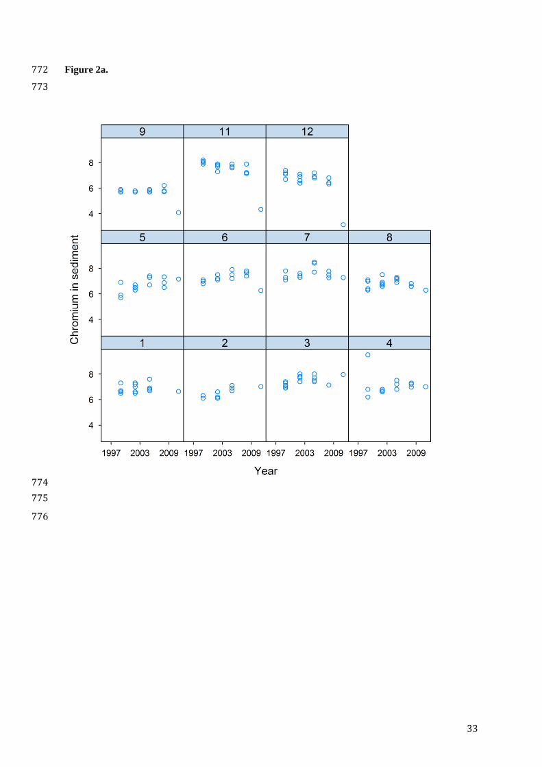
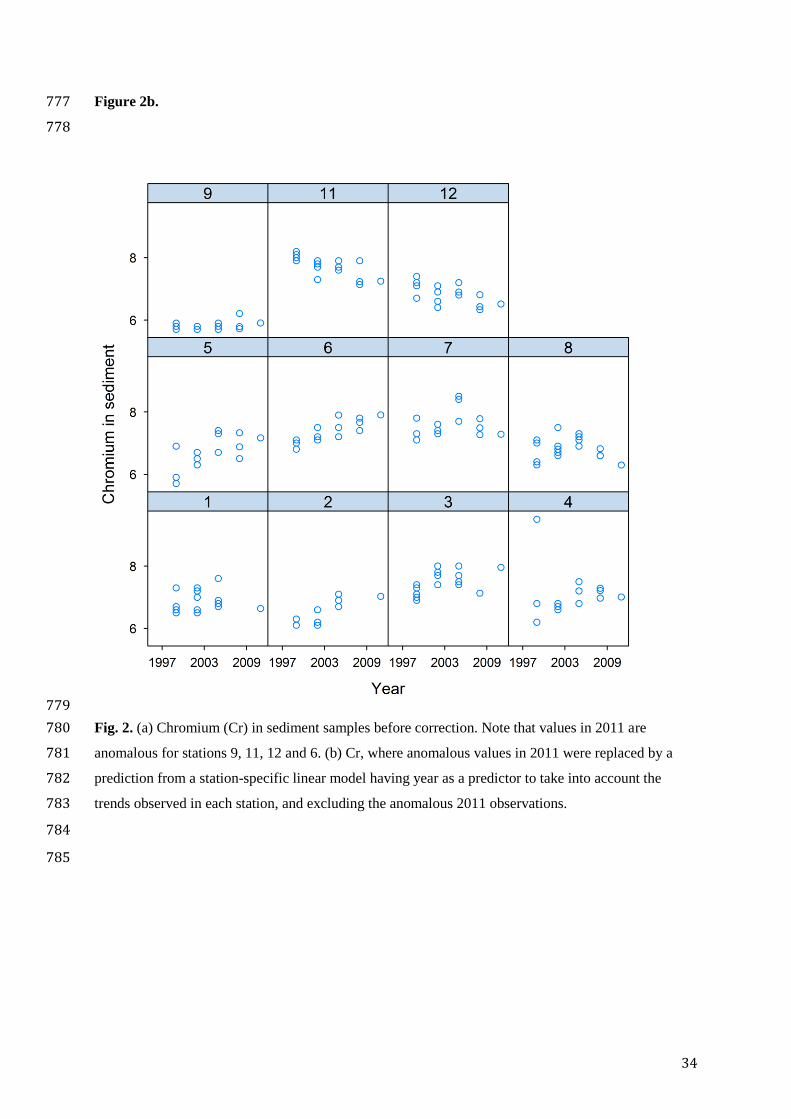
confirm this. Furthermore, values of Cr in the sediment samples from 2011 are anomalous for some 229
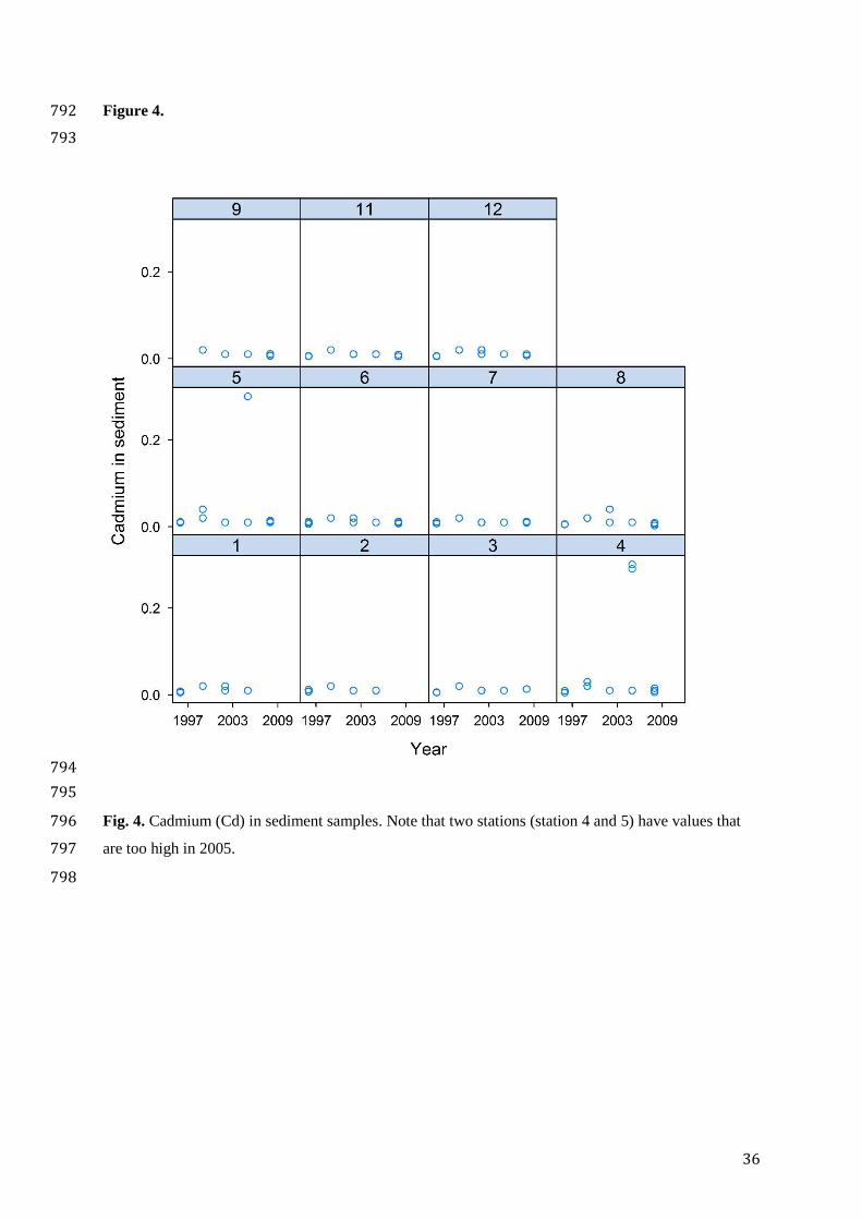
stations (stations 6, 9, 11, and 12, Fig. 2a). Ideally, such samples should have been rerun in the 230
laboratory immediately. When this has not been done, these values can be corrected prior to further 231
analyses, for example, by replacing them by a prediction from either a station-specific linear model 232
having year as a predictor to take into account the trends observed in each station, and excluding the 233
anomalous 2011 observations (as shown in Fig. 2b), or alternatively by a linear model for all stations 234
but including a year by station interaction. Such imputation of missing data can be taken into account 235
in latter analyses, as long as it is known which value is a direct measurement and which one is a 236
derived value (Little and Rubin 1987). Note that we have only Cr data from 4 sampling occasions 237
prior to 2011, so this correction should be checked when more data are available from future 238
monitoring. For Zn, the values in 2011 are anomalous at several stations (Fig. 3), and we have 239
therefore not included Zn in other analyses. Likewise, values of Cd in the sediment from 2005 for 240
stations 4 and 5 were significantly higher than in all other samples both in space and time (Fig. 4). We 241
have not included Cd in other analyses because there are few sampling occasions at several stations 242
(only 3 or 4 years if the year 1996 is not included). 243
10
244
In future we recommend that values are plotted immediately after laboratory analyses in order to 245
identify erroneous and missing values and rerun analyses when necessary. For environmental 246
variables, the replicates could be immediately plotted against the previous results (from other years 247
and other stations from the same year). If they do not show the same trend or fall outside a given 248
threshold (e.g. 2 SD) of the previous data, another subsample from each replicate could be done, and if 249
only one replicate lies outside, that replicate could be repeated. All data should be archived 250
irrespective of their anomalousness, as they might represent warning signals of change and not just 251
measurement errors. 252
253
For one station (station 9) from 1996 there was no faunal data given in the MOD-database. Likewise, 254
some sediment characteristics (e.g., fine sand, coarse sand, gravel, sediment median grain size, sorting, 255
skewness, and kurtosis) and some chemical variables (Cr, Cd, Cu, Fe, and Hg) were not measured on 256
all sampling occasions. One specific example of missing data is that median grain size was only given 257
for one station (station 9) from 1999 in the MOD-database. Raw data sheets may confirm if there were 258
no more samples analysed in 1999. Cr was not measured in 1996, but it can be included in temporal 259
analyses excluding this first year. For the years 1996, 2008 and 2011 values of “fine sand” are given in 260
the database, whereas for the other years values of “total sand” is given. Although most of the “total 261
sand” is “fine sand” this is obviously problematic for temporal analyses. In general, a relationship 262
between variables might be used to make predictions about missing values. However, lack of strong 263
relationships did not allow for any precise estimation of missing values in our case study. 264
265
Grooming the data will always be necessary, and some level of errors or problems with the data is 266
expected with regard to the size of this database (see also Hughes and Peck 2008). In the future, we 267
suggest that all data should be tested and corrected for errors before they are included in the MOD-268
database. It is much easier to resolve a problem in long-term data when it is identified in a timely 269
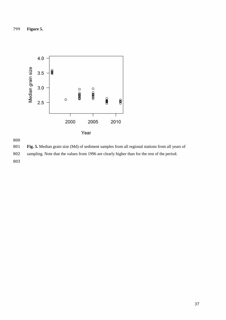
fashion and while observers and methods are still available for examination and discussion 270
(Lindenmayer and Likens 2010). With data included in a database, it is difficult to remember what 271
11
happened in the laboratory many years ago. When errors are identified, this should immediately be 272
reported to the organisation responsible for updating and maintaining the database. It is important to 273
immediately contact the laboratory responsible for the analyses and try to find out what might be the 274
reason for errors. Our findings highlight that the actual use of long-term data sets is the primary way 275
that errors, artefacts or other problems are uncovered (Lindenmayer and Likens 2010). Otherwise, 276
errors and inconsistencies may discourage thorough reanalysis. 277
278
The use of different laboratories over time 279
280
The sediment median grain size values from 1996 are clearly at a higher level than for the rest of the 281
sampling period (Fig. 5). This greatly influences the estimated trends; a linear mixed model with 282
station as a random factor and year as a fixed effect would result in a decrease per year of -0.062 (s.e. 283
= 0.0046), but removing 1996 more than halves the decrease to -0.028 (s.e. = 0.0031), with non-284
overlapping 95% confidence intervals. One particular laboratory was responsible for the analyses of 285
physical properties of the sediment in 1996, while different laboratories performed the analyses for 286
other years (Online Resource 1). As 1996 is the first year in this regional environmental monitoring 287
program, we have not included median grain size values from 1996 in further analyses of temporal 288
patterns. 289
290
We used data on TOM, fraction of silt and clay in the sediment, THC, PAH, Ba, Pb, and Cr for further 291
analyses of temporal patterns. We used Principal Component Analyses (PCA), using standardized 292
variables (subtracting the mean and dividing by the standard deviation). Replicates were first averaged 293
by station and year, and then standardized. The first PCA axis is a linear combination of the variables 294
maximizing the sum of squared correlations with all environmental variables. We therefore checked if 295
the different variables were approximately linearly correlated. To analyze change over time, we used 296
linear mixed models, with station and station by year as nested random factors. This allows for 297
dependency among observations made on the same station in a given year and of repeated 298
observations of the same station in different years, as well as estimating variance components 299

12
(repeated measurements of the same station in a given year, and stations over time). The analyses were 300
implemented in R, version 3.1.3 (R Core Team 2015). We used the libraries lme4 for linear mixed 301
models, and ade4 for PCA. 302
303
For a number of individual environmental variables (Ba, PAH, THC) where we had not already 304
identified any serious issues with the data (see above), the inclusion of the year 1996 in temporal 305
analyses turned out to be important for whether there was a trend in the data or not (Table 2). 306
Moreover, multivariate analyses based on a combined set of variables (TOM, silt-clay content, THC, 307
PAH, Ba and Pb) also revealed that 1996 was clearly separated from all following years of sampling 308
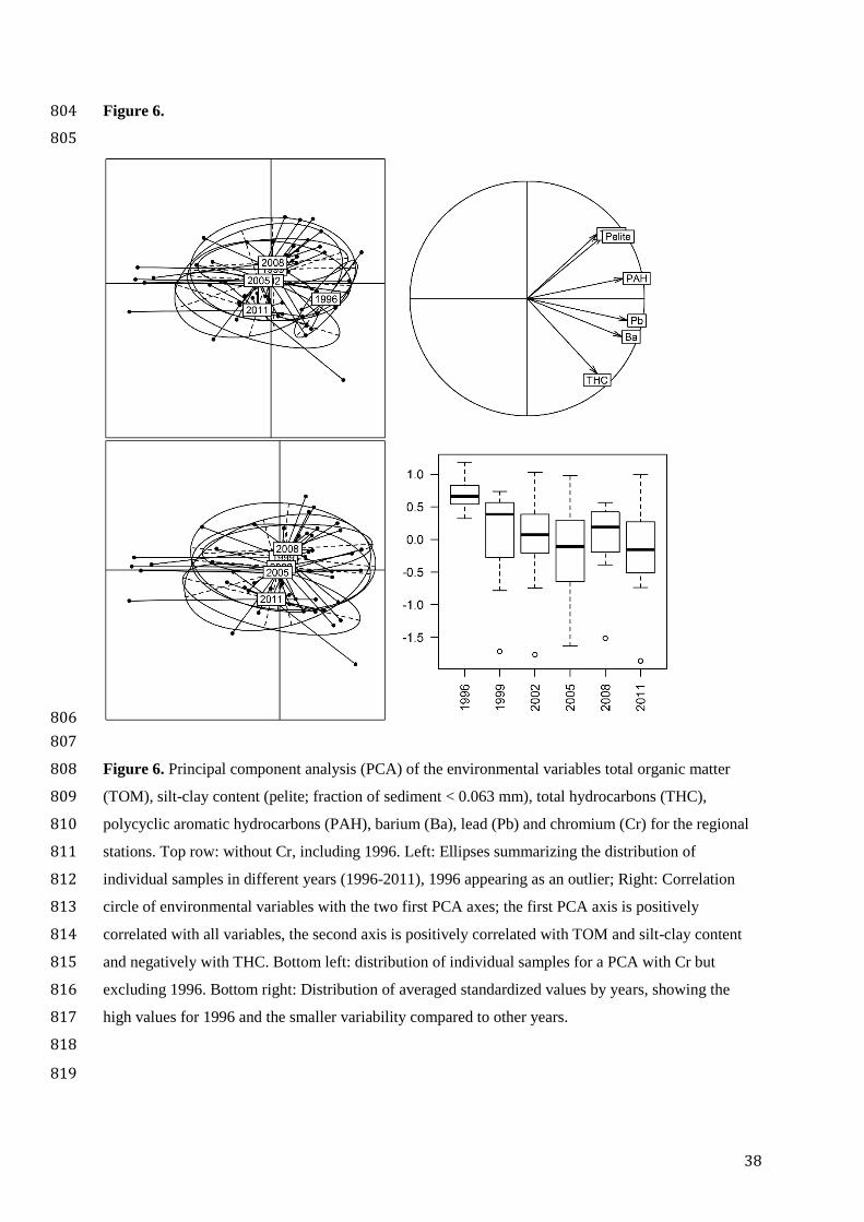
(Fig. 6), and this year had higher mean standardized values and lower variability than the following 309
years for the variables included in the analyses (Fig. 6). Importantly, in 1996, different laboratories 310
were used for sampling and analyses of both sediment organic chemistry, metals and physical 311
properties than for the next years (Online Resource 1). Note that if 1996 is omitted from the time 312
series, there is no clear trend in the data (Fig. 6). Although using a single laboratory to test all samples 313
may ensure consistency in the quality of results, it does not guarantee adequate quality. In this case, as 314
when several laboratories are participating in testing, it is imperative that inter-laboratory comparisons 315
are conducted (see Arrouays et al. 2012; Ross et al. 2015). Each year, some samples can be distributed 316
among the different laboratories that are involved in the monitoring over time. The results can then be 317
compared as a blind test each year. As an example, Ross et al. (2015) collected and distributed forest 318
soil samples to 15 laboratories in the eastern United States and Canada, and tested for variability 319
among laboratories for a number of soil properties. They recommended the continuation of reference 320
soil exchange programs to quantify the uncertainty associated with these analyses. Alternatively, 321
periodic analysis of reference samples is a widespread quality assurance procedure (Desaules 2012). 322
Replicate samples from the first sampling occasion or baseline study (site reference samples) can be 323
reanalysed simultaneously with the corresponding samples of each following sampling occasion. The 324
results can then be corrected based on the reanalysed first campaign samples, which correspond to a 325
site-specific control. This procedure would also enable different staff/laboratories to participate in the 326

13
long-term monitoring. However, it is important to evaluate issues of long-term storage effects on 327
measurements, and if this could complicate the analyses (see Ross et al. 2015). 328
329
Changes in protocols without calibration 330
331
Over time, there has been changes in the protocols of the Regional Monitoring. Because all the 332
datasets from the different years are collected in the MOD-database, and the changes in methods are 333
not flagged in the database, users may download data without knowledge about these changes. No 334
calibration has been done when protocols have been changed, i.e., running different protocols in 335
parallel, at least this information is not given in the database. The monitoring of TOM in the sediment 336
is one example of changes in procedures. From 2005, only one value was given for TOM in the MOD-337
database, because there was a change in procedure and sub-samples from three replicated grabs were 338
pooled prior to analyses instead of analysing the three replicates separately (Nøland et al. 2006). 339
Another example involves PAHs, which represent a group of compounds, and for the laboratory 340
analyses of PAHs in the sediment not every year has a description (either in the survey reports written 341
by the consulting companies or in the MOD-database) of exactly which compounds have been 342
analyzed and included in the term ‘PAH’ in the MOD-database. It is therefore unclear if these values 343
are comparable among years. Finally, only one replicate was analysed for metals in the sediments in 344
2011 compared to three or more replicates in previous years (Mannvik et al. 2012). This is particularly 345
problematic because values of some of the metals in the sediment samples from 2011, such as Cr and 346
Zn, are anomalous for several stations (see above, Fig. 2a, Fig. 3). It is not possible to decide if these 347
changes are caused by changes in the monitoring program or other factors. Importantly, modifying 348
methods can affect the ability to track changes in condition over repeated surveys (e.g. Hughes and 349
Peck 2008). If the protocols need to be changed, we recommend calibrating the new methods with the 350
previous methods, documenting the change and any effects on the measured variable (Lindenmayer 351
and Likens 2010; Lindenmayer et al. 2015), and giving information on this in the database. 352
353
The need for a modernisation of the MOD-database 354

14
355
In our case study, we have only focused on 11 stations from the MOD-database, however, our findings 356
are relevant for the entire Regional Monitoring. Importantly, a modification of the MOD-database 357
could hinder a number of errors and problems with the data, by for example not accepting errors in 358
species names, confusion with regard to (different) names of a given station or variable used for 359
different years, different level of information included in the database (e.g. “total sand” or “fine 360
sand”), and not accepting values larger or smaller than a given level. It could also take into account 361
changes in nomenclature over time. Currently, it takes more than 1.5 years after the data are collected 362
until they are included in the MOD-database (Iversen et al. 2015). Ideally, the data should be secured 363
in the MOD-database much more quickly. In our opinion, the MOD-database needs to be modernised 364
and restructured in order to secure the data in a better way and make the data more accessible for users 365
(including those processing the samples). Furthermore, we recommend that all analyses of data from 366
the Regional Monitoring, including the survey reports written by the consulting companies, should be 367
based on data downloaded from the (modified) MOD-database, and not from different databases 368
owned and controlled by the different consulting companies. 369
370
The importance of effective communication of knowledge can never be over emphasised. When the 371
knowledge is easy to access and openly available to all, including the management, industry, and the 372
public, this process will be more efficient. Interactive visualisation of data, analyses and results at 373
websites, can efficiently provide such information on environmental status and trends, with only 374
minimal effort of the user. We note that the construction of such interactive websites for long-term 375
monitoring data is currently rapidly increasing (Loraine et al. 2015), and we propose that the data 376
challenges outlined here could have been easily detected at an earlier stage if interactive tools for 377
analyses had been made available. 378
379
Uneven taxonomic resolution: potential consequences and recommendations 380
381

15
According to the current guidelines for the Regional Monitoring, the aim is that the taxa should be 382
identified to the species level, as far as possible (Iversen et al. 2015). All taxa collected during 383
sampling are included in the MOD-database, irrespective of the level of identification. For our case 384
study, 25% (98 of 388 taxa) of the data downloaded from the MOD-database were identified to a 385
coarser taxonomic level than species level, either at one or more sampling occasions. Over time, 386
different laboratories have been responsible for the species identification (Online Resource 1). 387
Consequently, taxa with “uncertain” classification (i.e. not identified to the species level) may vary 388
among years (and regions) if the competence of staff/laboratories differ. A taxon in a species list 389
extracted from the MOD-database can therefore appear as two different taxonomic units, and this 390
complicates the comparison of faunal patterns at stations over time (and space). 391
392
A new procedure to handle different taxonomic resolution 393
394
The large amount of historical data (since 1996) from the Regional Monitoring are highly valuable. 395
However, when we are using data from the MOD-database for scientific purpose, our aim is that 396
unidentified taxa should only be included in data analyses if they cannot be mistaken for other 397
identified species (or taxa in general). In earlier publications using data from the MOD-database, we 398
have subjectively processed the data prior to data analyses by either deleting or pooling taxa with 399
uncertain classifications (e.g., Ellingsen 2001; 2002; Ellingsen and Gray 2002). However, this 400
procedure is time consuming and, in addition, it is not easily repeatable for other users. Here we 401
present a new procedure, described and implemented in an R script, in order to transparently adjust the 402
faunal data with uncertain taxonomic classifications prior to data analyses. The procedure can be 403
illustrated using the two taxonomic levels genus and species. A genus can appear either as such (e.g., 404
Sphaerodorum spp) or as a species (e.g., Sphaerodorum gracilis). If there is only one species in a 405
genus, the genus can unambiguously be affected to the species, and either can be used. If there are 406
more than one species, we can consider two alternative solutions: alternative 1) “lumping” all species 407
in the genus and consider the genus as the only taxa, or alternative 2) removing observations appearing 408
only as genus and keep the species observations (“splitting”). The problem is that there are situations 409
16
where it makes sense to use the first alternative (e.g. first years appear only as genus, later years only 410
as many different species), whereas the second alternative may appear best in some cases (few 411
observations appear as genus and most as species). However, the first alternative may appear best if 412
most observations appear as genus and few as species, since removing the genus would remove much 413
information. We used the two approaches (lumping/splitting) in our case study to assess the sensitivity 414
of analyses to the two choices, but the most important is to make the choices transparent (and easily 415
modified if judged necessary) to assess the robustness of results. 416
417
Patterns of faunal composition – with and without correction of uncertain classifications 418
419
Prior to the data analyses, taxonomic groups not properly sampled by the methods used (Nematoda, 420
Foraminifera), colonial groups (Porifera, Hydrozoa, Bryozoa), pelagic crustaceans (Calanoida, 421
Mysidacea, Hyperiidae, Euphausiacea), and juveniles were excluded from the species list. Data 422
analyses were done on species abundance data at the replicate level. For our case study, the total 423
number of taxa in the unadjusted data set (i.e. directly downloaded from the MOD-database, but 424
excluding the taxonomic groups mentioned above) from all 11 regional stations and all six sampling 425
years was 388 taxa. The total number of taxa after adjusting for taxonomic classification uncertainties 426
was 294 (modification alternative 1, i.e. based on lumping) or 314 (modification alternative 2, i.e. 427
based on splitting). 428
429
We wanted to explore whether there were any differences in patterns of faunal composition based on 430
the unadjusted data vs the lumping/splitting data. In order to examine faunal composition over time 431
(and space) we used two approaches: Nonmetric Multidimensional Scaling (NMDS) using Bray-Curtis 432
distance to measure dissimilarity among samples (which corresponds to one station in a given year), 433
and Canonical Correspondence Analysis (CCA). We used both these analytical approaches because 434
both are commonly used when analyzing faunal composition, yet they are based on somewhat 435
different methodology. The analyses were implemented in R, version 3.1.3 (R Core Team 2015). We 436
used the libraries vegan for NMDS and ade4 for ordination analyses. 437

17
438
Using the unadjusted data set in the NMDS analysis clearly showed a separation between the years 439
1996, 1999-2002-2005, and 2008-2011 (Fig. 7). It is important to note that laboratory A was 440
responsible for sampling and taxa identification in 1996 and 2008-2011, whereas laboratory B was 441
responsible for the other three years (Online Resource 1). Because of this, it is difficult to ascertain if, 442
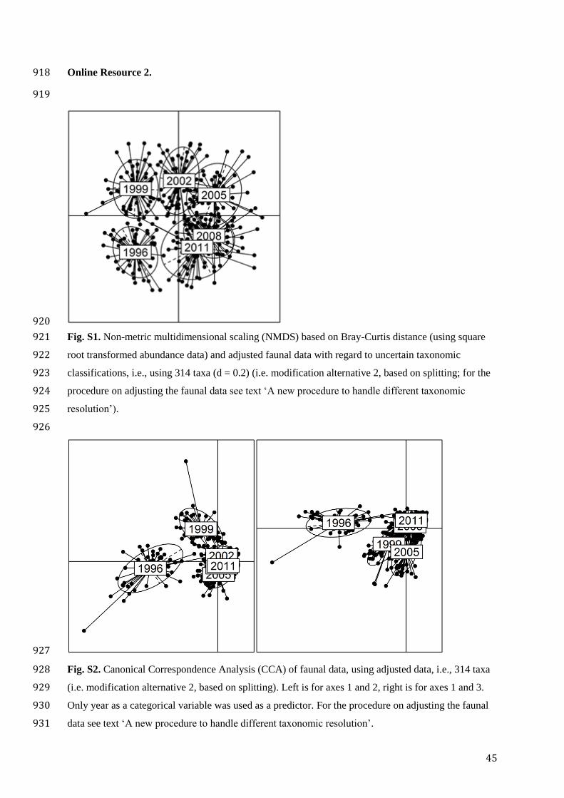
for example, there is a real difference between 1996 and the following years, or if this is a laboratory 443
effect. A CCA analysis based on the unadjusted faunal data also showed that the year 1996 was clearly 444
separated from all other years (Fig. 8), and this was even clearer than for the NMDS analysis (Fig. 7). 445
Within any laboratory, taxonomic competence can change over time, and among laboratories such 446
differences can be even larger. For the Regional Monitoring, this means that for one year a particular 447
taxon is identified to the species level, whereas for another year the same taxon may be identified to a 448
coarser taxonomic level, meaning that the taxon may be the same but it appears as different taxa for 449
the two years if data from these two years are combined. Some of the consultancy firms that perform 450
the Regional Monitoring have already speculated on potential effects of different practices. In a report 451
focusing on the period 1996-2006, Renaud et al. (2008) found strong inter-annual differences in 452
community structure, and suggested that this was likely due to changes in industry practices, as well as 453
natural variability in recruitment and mortality. Here we have illustrated the potential consequences of 454
comparing data among years (and laboratories) without considering the issue of stability and 455
taxonomic competence. 456
457
After applying our suggested new procedure for correcting the uncertain classifications, i.e. our 458
alternative 1 “lumping data” to 294 taxa, we see that the difference between 1999-2002-2005 and the 459
other years is not as large as for the unadjusted data (NMDS-plot, Fig. 7). Using our alternative 2 460
“splitting data”, we also found that the difference between 1999-2002-2005 and the other years is not 461
as large (NMDS, Online Resource 2). Likewise, using the adjusted “lumped” data set in the CCA 462
analysis showed that the faunal composition among years appear to be more similar than using the 463
unadjusted faunal data, although the first axis is still related to the separation between 1996 and all 464
other years (Fig. 8, for modification alternative 2 see Online Resource 2). This means that without 465
18
adjusting the data prior to the data analyses the years appear as more dissimilar to each other than what 466
they likely are. Yet, the differences were still substantial after adjustment. 467
468
For the shorter period from 1999 to 2005, when one laboratory was responsible for all three surveys, 469
there was a change in faunal composition from 1999 to 2002 to 2005 (Fig. 7). However, with only 470
three sampling occasions our ability to ascertain if this is a temporal trend is of course limited. Short 471
time series often constrain inferences about change because trend detection is limited by the number of 472
data points and temporal extent affecting whether a cyclic pattern is identified as a monotonic trend. 473
This requires a decision about how to treat trend detection involving consideration of the magnitude of 474
change vs statistical significance and the strong examination of patterns in residuals. 475
476
While we have suggested a procedure that takes into account the problem of uncertain species 477
identification in terms of data analysis, other options include taxonomists going back to archived 478
voucher specimens or image library. One alternative approach could also be to compare data at a 479
higher taxonomic level than at the species level (see e.g. Terlizzi et al. 2009; Fontaine et al. 2015), or 480
only focus on particular species or groups of species. However, we might expect the full community 481
identification to be more sensitive to identify community changes over space and time, although this 482
require further examination. 483
484
We have shown that the current procedures and, in particular, the use of different laboratories over 485
time strongly limit the utility of the historical data (since 1996) from the Norwegian continental shelf, 486
despite that the goal in the Regional Monitoring is to detect long-term trends and also provide an 487
estimate of the background conditions. Lindenmayer and Likens (2010) emphasize that several 488
seemingly small factors can contribute enormously to the success of long-term monitoring, sometimes 489
out of proportion to expectations. Stability and competence of staff is one such critical component, and 490
indeed, consistency increases comparability of data (Hughes and Peck 2008). Accordingly, 491
management of monitoring programmes that allow different companies to be responsible for 492
19
implementation over space or time, without extensive inter-calibration is not in accordance with the 493
current international recommendations (Arrouays et al. 2012). 494
495
Summary and recommendations 496
497
We have used a sub-set of data from a large-scale offshore regional environmental monitoring 498
program in Norway to explore concepts regarding best practices for long-term environmental 499
monitoring. The purpose of the Norwegian monitoring is to provide an overview of the environmental 500
status and trends in relation to the petroleum activities on the Norwegian continental shelf. Although, 501
there has been a focus on quality assurance/quality control protocols, we have identified a number of 502
challenges with regard to measurement inconsistencies, including discrepancies in variable and station 503
names, changes in procedures without proper calibration, different taxonomic resolution and changes 504
to nomenclature as well as missing values and outliers. Currently, it is difficult to decide if some of the 505
observed temporal changes at the stations in our case study are caused by natural variation, human 506
pressure, or simply by changes in the monitoring program over time, such as e.g. changes in 507
laboratory. We provide recommendations linked to these challenges to facilitate comparison of data 508
over time. We also present a new procedure, described and implemented in an R script, in order to 509
transparently adjust faunal data with uncertain taxonomic classifications prior to data analyses. Tightly 510
connected to these issues, we suggest that the data are carefully secured in a modernised database, 511
including that the data are constantly updated, regularly scrutinised for errors and rigorously reviewed, 512
and to make the data more accessible for users in Norway and elsewhere (see e.g. Fölster et al. 2014). 513
At present, a large part of the text in the database is given in Norwegian, which limit the availability 514
for international users. The construction of interactive websites for long-term monitoring data is 515
currently rapidly increasing, and we propose that the data challenges outlined here could have been 516
easily detected at an earlier stage if interactive tools for analyses were made available. Importantly, 517
frequent examination and use of data also result in important discoveries and stimulate new research 518
and management questions (Lindenmayer and Likens 2010). The Norwegian monitoring is an example 519
of a long-term monitoring program where reliable funding has been secured because the oil and gas 520
20
industry has a financial commitment. What is important is that the available resources are utilised in a 521
way that warrant both spatial and temporal comparisons. Furthermore, during the last decades it has 522
been a gradual change worldwide from a sectorial based monitoring (that is, with a focus on oil and 523
gas industry only) towards a more ecosystem-based monitoring. We advocate for revision and 524
updating of the Norwegian regional environmental monitoring program where potential multiple 525
stressor effects (e.g. bottom fishing, climate change) are used to inform the monitoring of the oil and 526
gas industry on the Norwegian continental shelf. This process would require a tight collaboration 527
between authorities, different industries and scientists. 528
529
References 530
531
Arrouays, D., Marchant, B. P., Saby, N. P. A., Meersmans, J., Orton, T. G., Martin, M. P., Bellamy, P. 532
H., Lark, R. M., & Kibblewhite, M. (2012). Generic issues on broad-scale soil monitoring schemes: a 533
review. Pedosphere, 22, 456-469. 534
535
Bakke, T., Green, A. M. V., & Iversen, P. E. (2011). Offshore environmental monitoring in Norway – 536
Regulations, results and developments. In K. Lee & J. Neff (Eds.), Produced Water (pp. 481-491). 537
Springer, NY (Chapter 25). 538
539
Bakke, T., Klungsøyr, J., & Sanni, S. (2013). Environmental impacts of produced water and drilling 540
waste discharges from the Norwegian offshore petroleum industry. Marine Environmental Research, 541
92, 154-169. 542
543
Bennett, J. R., Sisson, D. S., Smol, J. P., Cumming, B. F., Possingham, H. P., & Buckley, Y. M. 544
(2014). Optimizing taxonomic resolution and sampling effort to design cost-effective ecological 545
models for environmental assessment. Journal of Applied Ecology, 51, 1722-1732. 546
547

21
Buss, D. F., Carlisle, D. M., Chon, T.-S., Culp, J., Harding, J. S., Keizer-Vlek, H. E., et al., (2015). 548
Stream biomonitoring using macroinvertebrates around the globe: a comparison of large-scale 549
programs. Environmental Monitoring and Assessment, 187, 4132, doi: 10.1007/s10661-014-4132-8. 550
551
Cao, Y, & Hawkins, C. P. (2011). The comparability of bioassessments: a review of conceptual and 552
methodological issues. Journal of the North American Benthological Society, 30(3), 680-701. 553
554
Cochrane, S., Palerud, R., Wasbotten, I. H., Larsen, L. H., & Mannvik, H. P. (2009). Offshore 555
sediment survey of Region I, 2008. Akvaplan-niva report no. 4215 - 02. Akvaplan-niva, Tromsø, 556
Norway. 314 pp. 557
558
Desaules, A. (2012). Measurement instability and temporal bias in chemical soil monitoring: sources 559
and control measures. Environmental Monitoring and Assessment, 184, 487-502. 560
561
Ellingsen, K. E. (2001). Biodiversity of a continental shelf soft-sediment macrobenthos community. 562
Marine Ecology Progress Series, 218, 1-15. 563
564
Ellingsen, K. E. (2002). Continental shelf soft-sediment benthic biodiversity in relation to 565
environmental variability. Marine Ecology Progress Series, 232, 15-27. 566
567
Ellingsen, K. E., & Gray, J. S. (2002). Spatial patterns of benthic diversity: is there a latitudinal 568
gradient along the Norwegian continental shelf? Journal of Animal Ecology, 71, 373-389. 569
570
Fontaine, A., Devillers, R., Peres-Neto, P. R., & Johnson, L. E. (2015). Delineating marine ecological 571
units: a novel approach for deciding which taxonomic group to use and which taxonomic resolution to 572
choose. Diversity and Distributions, 21, 1167-1180. 573
574
22
Frid, C. L. J., Harwood, K. G., Hall, S. J., & Hall J. A. (2000). Long-term changes in the benthic 575
communities on North Sea fishing grounds. ICES Journal of Marine Science, 57, 1303-1309. 576
577
Fölster, J., Johnson, R. K., Futter, M. N., & Wilander, A. (2014). The Swedish monitoring of surface 578
waters: 50 years of adaptive monitoring. Ambio, 43, 3-18. 579
580
Gattuso, J.-P., Magnan, A., Billé, R., Cheung, W. W. L., Howes, E. L., Joos, F., et al., (2015). 581
Contrasting futures for ocean and society from different anthropogenic CO2 emissions scenarios. 582
Science, 349. 583
584
Gray, J. S., Clarke, K. R., Warwick, R. M., & Hobbs, G. (1990). Detection of initial effects of 585
pollution on marine benthos: an example from the Ekofisk and Eldfisk oilfields, North Sea. Marine 586
Ecology Progress Series, 66, 285-299. 587
588
Gray, J. S., Bakke, T., Beck, H. J., & Nilssen, I. (1999). Managing the environment effects of the 589
Norwegian oil and gas industry: from conflict to consensus. Marine Pollution Bulletin, 38(7), 525-590
530. 591
592
Hewitt, J. E., & Thrush, S. F. (2007). Effective long-term ecological monitoring using spatially and 593
temporally nested sampling. Environmental Monitoring and Assessment, 133, 295-307. 594
595
Hughes, B. (2014). Monitoring: Garbage In Yields Garbage Out. Fisheries, 39(6), 243-243, doi: 596
10.1080/03632415.2014.915813. 597
598
Hughes, R. M., & Peck, D. V. (2008). Acquiring data for large aquatic resource surveys: the art of 599
compromise among science, logistics, and reality. Journal of the North American Benthological 600
Society, 27(4), 837-859. 601
602

23
Iversen, P. E., Green, A. M. V., Lind, M. J., Petersen, M. R. H., Bakke, T., Lichtenthaler, R., et al., 603
(2011). Guidelines for offshore environmental monitoring: The petroleum sector on the Norwegian 604
Continental Shelf. Climate and Pollution Agency. TA number 2849/2011. 49 pp. 605
606
Iversen, P. E. Lind, M. J., Ersvik, M., Rønning, I., Skaare, B. B., Green, A. M. V., et al., (2015). 607
Guidelines for environmental monitoring of petroleum activities on the Norwegian continental shelf. 608
The Norwegian Environment. Agency M-number M-300/2015. 60 pp. (In Norwegian) 609
610
Jensen, T., Gjøs, N., Nøland, S.-A., Oreld, F., Møskeland, T., Bakke, S. M., et al., (2000). 611
Environmental Monitoring 1999, Region I – Ekofisk. Technical Report. Report no. 2000-3238. Det 612
Norske Veritas & Sintef Applied Chemistry, Norway. 294 pp. 613
614
Kaiser, M. J., Clarke, K. R., Hinz, H., Austen, M. C. V., Somerfield, P. J., & Karakassis, I. (2006). 615
Global analysis of response and recovery of benthic biota to fishing. Marine Ecology Progress Series, 616
311, 1-14. 617
618
Lindenmayer, D. B., Burns, E. L., Tennant, P., Dickman, C. R., Green, P.T., Keith, D. A., et al., 619
(2015). Contemplating the future: Acting now on long-term monitoring to answer 2050’s questions. 620
Austral Ecology, 40, 213-224. 621
622
Lindenmayer, D. B., & Likens, G. E. (2010). Effective ecological monitoring. CSIRO Publishing, 623
London, 170 pp. 624
625
Little, R. J. A., & Rubin, D. B. (1987). Statistical analysis with missing data. John Wiley and Sons, 626
New York. 627
628

24
Loraine, A. E., Blakley, I. C., Jagadeesan, S., Harper, J., Miller, G., & Firon, N. (2015). Analysis and 629
visualization of RNA-Seq expression data using RStudio, Bioconductor, and Integrated Genome 630
Browser. Methods in molecular biology (Clifton, N. J.), 1284, 481-501. 631
632
Mannvik, H. P., Pearson, T., Pettersen, A., & Lie Gabrielsen, K. (1997). Environmental monitoring 633
survey Region I 1996. Main Report. Akvaplan-niva report no. 411.96.996-1. Akvaplan-Niva, Tromsø, 634
Norway. 246 pp. 635
636
Mannvik, H. P., Wasbotten, I. H., Cochrane, S., & Moldes-Anaya, A. (2012). Miljøundersøkelse 637
Region I, 2011. Akvaplan-niva report no. 5339.02. Akvaplan-niva, Tromsø, Norway. 196 pp. (In 638
Norwegian). 639
640
Mieszkowska, N., Sugden, H., Firth, L. B., & Hawkins, S. J. (2014). The role of sustained 641
observations in tracking impacts of environmental change on marine biodiversity and ecosystems. 642
Philosophical Transactions of the Royal Society A, 372, 20130339. 643
644
Nichols, J. D., & Williams, B. K. (2006). Monitoring for conservation. Trends in Ecology & 645
Evolution, 21, 668-673. 646
647
Norwegian Oil and Gas (2013). Environmental Report 2013. The Norwegian Oil and Gas Association. 648
http://www.norskoljeoggass.no/en/Publica/Environmentalreports/Environmental-report-2013/. 649
650
Nøland, S. A., Gjøs, N., Bakke, S. M., & Oreld F. (2003). Environmental Monitoring 2002, Region I – 651
Ekofisk. Main report. Technical Report. Report no. 2003-0338. Det Norske Veritas/Sintef, Norway. 652
316 pp. 653
654
Nøland, S. A., Bakke, S. M., Rustad, I., & Brinchmann, K. M. (2006). Environmental Monitoring 655
Region I, 2005. Main Report. Report no. 2006-0187. Det Norske Veritas, Norway. 344 pp. 656

25
657
Olsgard, F., & Gray, J.S. (1995). A comprehensive analysis of the effects of offshore oil and gas 658
exploration and production on the benthic communities of the Norwegian continental shelf. Marine 659
Ecology Progress Series, 122, 277-306. 660
661
R Core Team (2015). R: A language and environment for statistical computing. R Foundation for 662
Statistical Computing, Vienna, Austria. URL http://www.R-project.org/. 663
664
Renaud, P. E., Jensen, T., Wassbotten, I., Mannvik, H. P., & Botnen, H., (2008). Offshore sediment 665
monitoring on the Norwegian shelf. A regional approach 1996-2006. Akvaplan-niva report no 3487 – 666
003. Akvaplan-Niva, Tromsø, Norway. 95 pp. 667
668
Ross, D.S., Bailey, S.W., Briggs, R.D., Curry, J., Fernandez, I.J., Fredriksen, G., et al., (2015). Inter-669
laboratory variation in the chemical analysis of acidic forest soil reference samples from eastern North 670
America. Ecosphere, 6(5), 73. http://dx.doi.org/10.1890/ES14-00209.1. 671
672
Terlizzi, A., Anderson, M. J., Bevilacqua, S., Fraschetti, S., Wlodarska-Kowalcuk, M., & Ellingsen, 673
K. E. (2009). Beta diversity and taxonomic sufficiency: Do higher-level taxa reflect heterogeneity in 674
species composition? Diversity and Distributions, 15, 450-458. 675
676
Thrush, S. F., & Dayton, P. K. (2002). Disturbance to marine benthic habitats by trawling and 677
dredging: implications for marine biodiversity. Annual Review of Ecology and Systematics, 33, 449-678
473. 679
680
Thrush, S. F., Ellingsen, K. E., & Davis, K. (2015). Implications of fisheries impacts to seafloor 681
biodiversity and Ecosystem-Based Management. ICES Journal of Marine Science, 73 (Supplement 1), 682
i44-i50, doi:10.1093/icesjms/fsv114. 683
684

26
Yoccoz, N. G., Nichols, J. D., & Boulinier, T. (2001). Monitoring of biological diversity in space and 685
time. TRENDS in Ecology & Evolution, 16, 446-453. 686
687
27
Figure legends 688
689
Fig. 1. Overview and location of 11 regional stations (red circles) and the petroleum installations 690
(stars) in Region I (Ekofisk) on the southern part of the Norwegian continental shelf, in the North Sea. 691
692
Fig. 2. (a) Chromium (Cr) in sediment samples before correction. Note that values in 2011 are 693
anomalous for stations 9, 11, 12 and 6. (b) Cr, where anomalous values in 2011 were replaced by a 694
prediction from a station-specific linear model having year as a predictor to take into account the 695
trends observed in each station, and excluding the anomalous 2011 observations. 696
697
Fig. 3. Zinc (Zn) in sediment samples. Note that there is a trend in the data prior to 2011 at several 698
stations, but that the values in 2011 are lower. There is only one replicate in 2011. 699
700
Fig. 4. Cadmium (Cd) in sediment samples. Note that two stations (station 4 and 5) have values that 701
are too high in 2005. 702
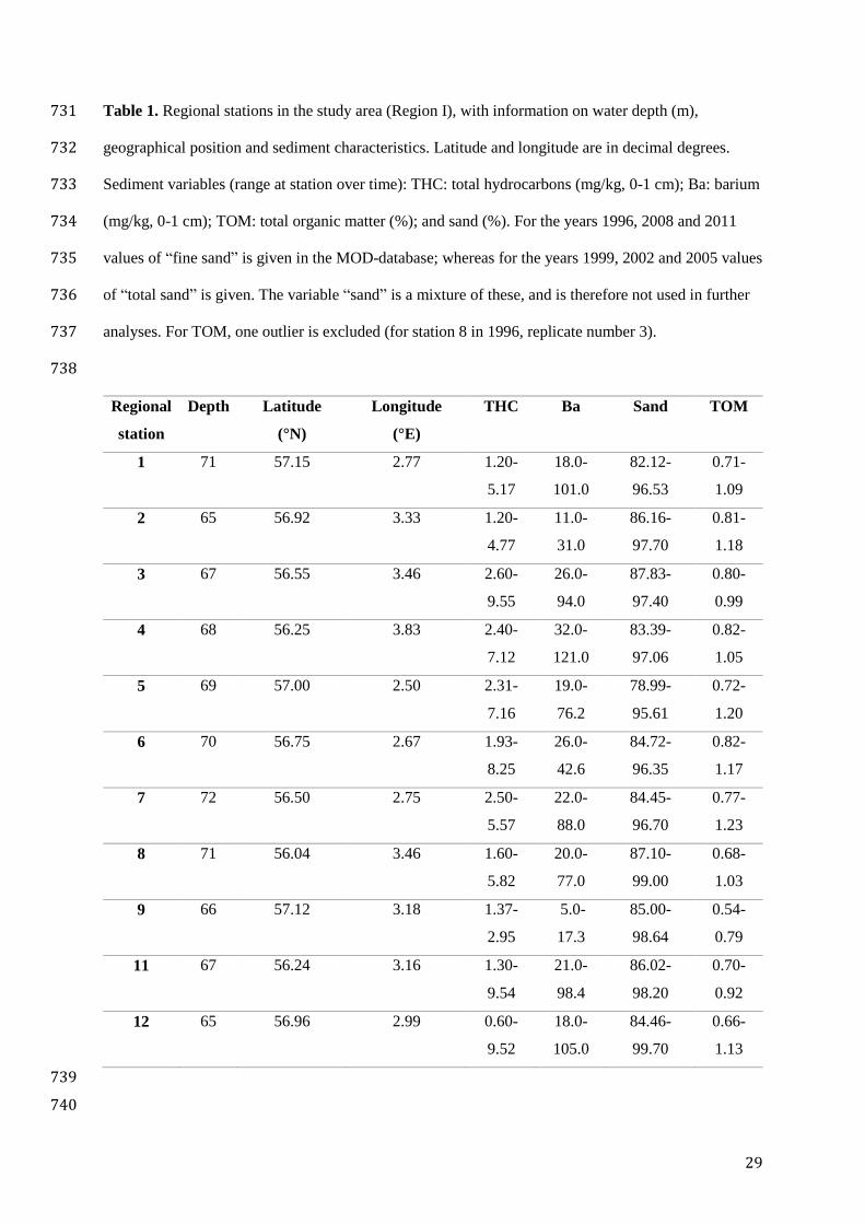
703
Fig. 5. Median grain size (Md) of sediment samples from all regional stations from all years of 704
sampling. Note that the values from 1996 are clearly higher than for the rest of the period. 705
706
Fig. 6. Principal component analysis (PCA) of the environmental variables total organic matter 707
(TOM), silt-clay content (pelite; fraction of sediment < 0.063 mm), total hydrocarbons (THC), 708
polycyclic aromatic hydrocarbons (PAH), barium (Ba), lead (Pb) and chromium (Cr) for the regional 709
stations. Top row: without Cr, including 1996. Left: Ellipses summarizing the distribution of 710
individual samples in different years (1996-2011), 1996 appearing as an outlier; Right: Correlation 711

28
circle of environmental variables with the two first PCA axes; the first PCA axis is positively 712
correlated with all variables, the second axis is positively correlated with TOM and silt-clay content 713
and negatively with THC. Bottom left: distribution of individual samples for a PCA with Cr but 714
excluding 1996. Bottom right: Distribution of averaged standardized values by years, showing the 715
high values for 1996 and the smaller variability compared to other years. 716
717
Fig. 7. Non-metric multidimensional scaling (NMDS) based on Bray-Curtis distance (using square 718
root transformed abundance data) and unadjusted faunal data, i.e. 388 taxa (d = 0.5) (left), and 719
adjusted faunal data with regard to uncertain taxonomic classifications, i.e., 294 taxa (modification 720
alternative 1, based on “lumping”) (d = 0.2) (right). For the procedure on adjusting the faunal data see 721
text ‘A new procedure to handle different taxonomic resolution’. 722
723
Fig. 8. Canonical Correspondence Analysis (CCA) of faunal data, left on unadjusted data, i.e. 388 724
taxa, right on adjusted data, i.e., 294 taxa (modification alternative 1, based on “lumping”). Top is for 725
axes 1 and 2, bottom is for axes 1 and 3. Only year as a categorical variable was used as a predictor. 726
For the procedure on adjusting the faunal data see text ‘A new procedure to handle different 727
taxonomic resolution’. 728
729
730
29
Table 1. Regional stations in the study area (Region I), with information on water depth (m), 731
geographical position and sediment characteristics. Latitude and longitude are in decimal degrees. 732
Sediment variables (range at station over time): THC: total hydrocarbons (mg/kg, 0-1 cm); Ba: barium 733
(mg/kg, 0-1 cm); TOM: total organic matter (%); and sand (%). For the years 1996, 2008 and 2011 734
values of “fine sand” is given in the MOD-database; whereas for the years 1999, 2002 and 2005 values 735
of “total sand” is given. The variable “sand” is a mixture of these, and is therefore not used in further 736
analyses. For TOM, one outlier is excluded (for station 8 in 1996, replicate number 3). 737
738
Regional
station
Depth Latitude
(°N)
Longitude
(°E)
THC Ba Sand TOM
1 71 57.15 2.77 1.20-
5.17
18.0-
101.0
82.12-
96.53
0.71-
1.09
2 65 56.92 3.33 1.20-
4.77
11.0-
31.0
86.16-
97.70
0.81-
1.18
3 67 56.55 3.46 2.60-
9.55
26.0-
94.0
87.83-
97.40
0.80-
0.99
4 68 56.25 3.83 2.40-
7.12
32.0-
121.0
83.39-
97.06
0.82-
1.05
5 69 57.00 2.50 2.31-
7.16
19.0-
76.2
78.99-
95.61
0.72-
1.20
6 70 56.75 2.67 1.93-
8.25
26.0-
42.6
84.72-
96.35
0.82-
1.17
7 72 56.50 2.75 2.50-
5.57
22.0-
88.0
84.45-
96.70
0.77-
1.23
8 71 56.04 3.46 1.60-
5.82
20.0-
77.0
87.10-
99.00
0.68-
1.03
9 66 57.12 3.18 1.37-
2.95
5.0-
17.3
85.00-
98.64
0.54-
0.79
11 67 56.24 3.16 1.30-
9.54
21.0-
98.4
86.02-
98.20
0.70-
0.92
12 65 56.96 2.99 0.60-
9.52
18.0-
105.0
84.46-
99.70
0.66-
1.13
739
740

30
Table 2. Estimates of linear yearly trends of environmental variables (with se in parenthesis) obtained 741
with a linear mixed model with station and station by year random effects. Statistically linear trends 742
(at the 0.05 level) are indicated in bold/italics. TOM: total organic matter (%); Ba: barium; PAH: 743
polycyclic aromatic hydrocarbons; THC: total hydrocarbons. 744
745
Variables With 1996 Without 1996
TOM -0.0069 (0.0022) -0.0090 (0.0029)
Ba -0.67 (0.32) 0.43 (0.35)
PAH (x1000) -0.72 (0.29) 0.0 (0.25)
THC -0.098 (0.026) -0.032 (0.032)
746
747
31
Data accessibility: Faunal data and a description of the procedure of lumping/splitting taxa in the 748
species list prior to data analyses (including the R script) will be made available from the Dryad 749
Digital Repository after publication. 750
751
Supplementary Information 752
Additional Supporting Information may be found in the online version of this article. 753
754
Online Resource 1. 755
Table S1. Consulting companies responsible for fieldwork, identification of taxa, and laboratory 756
analyses. 757
758
Online Resource 2. 759
Fig. S1. Non-metric multidimensional scaling (NMDS) using faunal data based on the splitting 760
procedure. 761
Fig. S2. Canonical Correspondence Analysis (CCA) using faunal data based on the splitting 762
procedure. 763
764
765

32
Figure 1. 766
767
768
Fig. 1. Overview and location of 11 regional stations (red circles) and the petroleum installations 769
(stars) in Region I (Ekofisk) on the southern part of the Norwegian continental shelf, in the North Sea. 770
771
33
Figure 2a. 772
773
774
775
776
34
Figure 2b. 777
778
779
Fig. 2. (a) Chromium (Cr) in sediment samples before correction. Note that values in 2011 are 780
anomalous for stations 9, 11, 12 and 6. (b) Cr, where anomalous values in 2011 were replaced by a 781
prediction from a station-specific linear model having year as a predictor to take into account the 782
trends observed in each station, and excluding the anomalous 2011 observations. 783
784
785

35
Figure 3. 786
787
Fig. 3. Zinc (Zn) in sediment samples. Note that there is a trend in the data prior to 2011 at several 788
stations, but that the values in 2011 are lower. There is only one replicate in 2011. 789
790
791
36
Figure 4. 792
793
794
795
Fig. 4. Cadmium (Cd) in sediment samples. Note that two stations (station 4 and 5) have values that 796
are too high in 2005. 797
798
37
Figure 5. 799
800
Fig. 5. Median grain size (Md) of sediment samples from all regional stations from all years of 801
sampling. Note that the values from 1996 are clearly higher than for the rest of the period. 802
803
38
Figure 6. 804
805
806
807
Figure 6. Principal component analysis (PCA) of the environmental variables total organic matter 808
(TOM), silt-clay content (pelite; fraction of sediment < 0.063 mm), total hydrocarbons (THC), 809
polycyclic aromatic hydrocarbons (PAH), barium (Ba), lead (Pb) and chromium (Cr) for the regional 810
stations. Top row: without Cr, including 1996. Left: Ellipses summarizing the distribution of 811
individual samples in different years (1996-2011), 1996 appearing as an outlier; Right: Correlation 812
circle of environmental variables with the two first PCA axes; the first PCA axis is positively 813
correlated with all variables, the second axis is positively correlated with TOM and silt-clay content 814
and negatively with THC. Bottom left: distribution of individual samples for a PCA with Cr but 815
excluding 1996. Bottom right: Distribution of averaged standardized values by years, showing the 816
high values for 1996 and the smaller variability compared to other years. 817
818
819

39
Figure 7. 820
821
822
823
Fig. 7. Non-metric multidimensional scaling (NMDS) based on Bray-Curtis distance (using square 824
root transformed abundance data) and unadjusted faunal data, i.e. 388 taxa (d = 0.5) (left), and 825
adjusted faunal data with regard to uncertain taxonomic classifications, i.e., 294 taxa (modification 826
alternative 1, based on “lumping”) (d = 0.2) (right). For the procedure on adjusting the faunal data see 827
text ‘A new procedure to handle different taxonomic resolution’. 828
829
40
Figure 8. 830
831
832
833
Fig. 8. Canonical Correspondence Analysis (CCA) of faunal data, left on unadjusted data, i.e. 388 834
taxa, right on adjusted data, i.e., 294 taxa (modification alternative 1, based on “lumping”). Top is for 835
axes 1 and 2, bottom is for axes 1 and 3. Only year as a categorical variable was used as a predictor. 836
For the procedure on adjusting the faunal data see text ‘A new procedure to handle different 837
taxonomic resolution’. 838
839
840

41
Supplementary information. Table. 841
842
Article title: Long-term environmental monitoring for assessment of change: measurement 843
inconsistencies over time and potential solutions 844
845
Journal name: Environmental Monitoring and Assessment 846
847
Author names: Kari E. Ellingsen1*, Nigel G. Yoccoz1,2, Torkild Tveraa1, Judi E. Hewitt3 and Simon 848
F. Thrush4 849
850
1 Norwegian Institute for Nature Research (NINA), Fram Centre, P.O. Box 6606 Langnes, 9296 851
Tromsø, Norway 852
853
2 Department of Arctic and Marine Biology, UiT The Arctic University of Norway, 9037 Tromsø, 854
Norway 855
856
3 National Institute of Water and Atmospheric Research, NZ 857
858
4 Institute of Marine Sciences, University of Auckland, NZ 859
860
* Corresponding author: E-mail: [email protected] 861
862

42
Online Resource 1. 863
864
Table S1. Consulting companies (identified by letters) responsible for fieldwork during each sampling 865
occasion, identification of taxa, and analyses of organic chemistry, metals and physical properties of 866
the sediment samples. For further information, see survey reports written by consulting companies 867
(Cochrane et al. 2009; Jensen et al. 2000; Mannvik et al. 1997; Mannvik et al. 2012; Nøland et al. 868
2003; Nøland et al.2006). 869
Year Field work Taxa
identification
Analyses of sediment in laboratory
Main responsible Organic
chemistry
Metals Physical
properties
1996 A, C A C G F
1999 B, D B D D D
2002 B, D B D D D
2005 B, E B E E E
2008 A, C A C G C
2011 A, C A C H C
870
References 871
Cochrane, S., Palerud, R., Wasbotten, I. H., Larsen, L. H., & Mannvik, H. P. (2009). Offshore 872
sediment survey of Region I, 2008. Akvaplan-niva report no. 4215 - 02. Akvaplan-niva, Tromsø, 873
Norway. 314 pp. 874
875
Jensen, T., Gjøs, N., Nøland, S.-A., Oreld, F., Møskeland, T., Bakke, S. M., et al., (2000). 876
Environmental Monitoring 1999, Region I – Ekofisk. Technical Report. Report no. 2000-3238. Det 877
Norske Veritas & Sintef Applied Chemistry, Norway. 294 pp. 878
879
Mannvik, H. P., Pearson, T., Pettersen, A., & Lie Gabrielsen, K. (1997). Environmental monitoring 880
survey Region I 1996. Main Report. Akvaplan-niva report no. 411.96.996-1. Akvaplan-Niva, Tromsø, 881
Norway. 246 pp. 882
883
Mannvik, H. P., Wasbotten, I. H., Cochrane, S., & Moldes-Anaya, A. (2012). Miljøundersøkelse 884
Region I, 2011. Akvaplan-niva report no. 5339.02. Akvaplan-niva, Tromsø, Norway. 196 pp. (In 885
Norwegian). 886
887

43
Nøland, S. A., Gjøs, N., Bakke, S. M., & Oreld F. (2003). Environmental Monitoring 2002, Region I – 888
Ekofisk. Main report. Technical Report. Report no. 2003-0338. Det Norske Veritas/Sintef, Norway. 889
316 pp. 890
891
Nøland, S. A., Bakke, S. M., Rustad, I., & Brinchmann, K. M. (2006). Environmental Monitoring 892
Region I, 2005. Main Report. Report no. 2006-0187. Det Norske Veritas, Norway. 344 pp. 893
894
895

44
Supplementary information. Figures. 896
897
Article title: Long-term environmental monitoring for assessment of change: measurement 898
inconsistencies over time and potential solutions 899
900
Journal name: Environmental Monitoring and Assessment 901
902
Author names: Kari E. Ellingsen1*, Nigel G. Yoccoz1,2, Torkild Tveraa1, Judi E. Hewitt3 and Simon 903
F. Thrush4 904
905
1 Norwegian Institute for Nature Research (NINA), Fram Centre, P.O. Box 6606 Langnes, 9296 906
Tromsø, Norway 907
908
2 Department of Arctic and Marine Biology, UiT The Arctic University of Norway, 9037 Tromsø, 909
Norway 910
911
3 National Institute of Water and Atmospheric Research, NZ 912
913
4 Institute of Marine Sciences, University of Auckland, NZ 914
915
* Corresponding author: E-mail: [email protected] 916
917
45
Online Resource 2. 918
919
920
Fig. S1. Non-metric multidimensional scaling (NMDS) based on Bray-Curtis distance (using square 921
root transformed abundance data) and adjusted faunal data with regard to uncertain taxonomic 922
classifications, i.e., using 314 taxa (d = 0.2) (i.e. modification alternative 2, based on splitting; for the 923
procedure on adjusting the faunal data see text ‘A new procedure to handle different taxonomic 924
resolution’). 925
926
927
Fig. S2. Canonical Correspondence Analysis (CCA) of faunal data, using adjusted data, i.e., 314 taxa 928
(i.e. modification alternative 2, based on splitting). Left is for axes 1 and 2, right is for axes 1 and 3. 929
Only year as a categorical variable was used as a predictor. For the procedure on adjusting the faunal 930
data see text ‘A new procedure to handle different taxonomic resolution’. 931