Embed Size (px)
Citation preview

Wages Rents and the Quality of Life
Jennifer Roback
The Journal of Political Economy Vol 90 No 6 (Dec 1982) pp 1257-1278
Stable URL
httplinksjstororgsicisici=0022-38082819821229903A63C12573AWRATQO3E20CO3B2-7
The Journal of Political Economy is currently published by The University of Chicago Press
Your use of the JSTOR archive indicates your acceptance of JSTORs Terms and Conditions of Use available athttpwwwjstororgabouttermshtml JSTORs Terms and Conditions of Use provides in part that unless you have obtainedprior permission you may not download an entire issue of a journal or multiple copies of articles and you may use content inthe JSTOR archive only for your personal non-commercial use
Please contact the publisher regarding any further use of this work Publisher contact information may be obtained athttpwwwjstororgjournalsucpresshtml
Each copy of any part of a JSTOR transmission must contain the same copyright notice that appears on the screen or printedpage of such transmission
The JSTOR Archive is a trusted digital repository providing for long-term preservation and access to leading academicjournals and scholarly literature from around the world The Archive is supported by libraries scholarly societies publishersand foundations It is an initiative of JSTOR a not-for-profit organization with a mission to help the scholarly community takeadvantage of advances in technology For more information regarding JSTOR please contact supportjstororg
httpwwwjstororgWed Aug 22 040913 2007
Wages Rents and the Quality of Life
Jennifer Roback k1( l I I Z ~ I h
Ihis ~ t u d v focuses on the role of ages and rents in allocating orkels to locations ith valious quantities of rmenitie5 The theory denlollstl-ate5 that if the amenity is also pi-od~~ctive tllerl the sign of the -age gladient is unclear bile the rent gr~dient is positire The tlleor is extended to include the housing market and nonti-add goods Ihese extensiorls require little modification of the conclusion 1-he elllpilicil rvo1k on liages shois that the I-egional age dif- lelences ~ 2 1 1 11)e explained lal-gel by these locrl lttributes Vith the
of jitt price diti irnplicit 111-ice ire estirn~ted and c1ullitv of l i t+ rankings h l - the cities are computed
Introduction
Ihe pl-ohlern o f co11-ectly measur ing t h e implicit price of u r b a n iitt1i- [lutes has 1eceived rnuch at tention in the past decade hlost o f t h e studies have used some variant o f t h e hedonic price m e t h o d e i ther estimating lage differentials (hrol dhaus a n d Ipbin 1972 Getz a n d H u a n g 1978 Rosen 1979) ol- est imating r en t differentials (Ridkel- a n d H e n n i n g 1967 Polinsky a n d Ruhinfeld 1977) Unfol-tunately these studies have focused solely o n the consumel s ide of t he marke t vi t l iout any r ega rd given to the behaviol- of firrns F o r example if t-o~-kelsrequil-e a cornpensating wage differential to live in a big polluted or otherwise unpleiisant city t h e f irms in tha t city must have
1 oul(l like to t h n k She~rti Roseti Elhatian Helpmati and the Ltiie~-sitv of (h~cao pplications of Economic Val kshop tor helpful corlilnetits This 111ate1-ial is I)~sedon ~to1k supported ty Scietice Fo~~tidation the N~ t io t i ~ l undel gl-ant S 0 ( 7 7 -24282 n v opinions findings and conclusions or ~ecorlirliend~tioti in th~sep~essed pul)lic~tion21-e rnine and do not necessi~-ily r-eflect the ies of the Nrtion~l Scrence Founcl~tioll1 ilso henetited g~eitlr fr-om the estensie corliments of the r-ekree
some pl-oductivity advantage to be able to pay the higher tvage Indeed one of the chief insights of Kosens ( 1 974) theoretical tvol-k on hedonic prices is that the implicit price of an attribute represents both the rnal-ginal valuation to consumers and the marginal cost to firms Thus i f one ignores the firm side of the market the rnatcliing aspect of the pioblern has heen lost
If one seriously considers a full hedonic rnodel of the intercity location problern one discovel-s that the prohle~n is much more for- midable than the usual hedonic price pl-ohlern because both the land and the labol- rnarkets must clear A simple example will illustrate the difficulty Suppose all firms and all tvorkers are identical Then the usual result is that only one type ofjoh 01- one brand of product will he offel-eti This presents no problem if the good undel consideration is a refl-igelitol- 01 a car because all consurnel-s may certainly consurne the sarne type of refrigel-atol- if they so desire Hotvever in the spatial allocation pr-oblern people cannot all occupy the same space even if their preferences are identical Hence the scarcity of amenable land gives rise to an additional constl-aint on the p1ohlern T h e already difficult pl-oblern of solving explicitly for a hedonic price equilibrium becomes all but impossible when ttvo rnarkets must clear simultane- ously
T h e preceding discussion illustrates t~vo major outstanding proh- lerns in this field Fir-t the role of the interconnected land and lat~or rnu-ket-clearing conditions in generating the equilihriurn is not ~vell undelstood Second the tictors which influence the precise decom- position of the implicit prices into wage and rent gradients have not been detel-mined T h e present tvork addresses these questions by using a general equilibr-iu~n model tvhich incorpo~ates both rnobile flctors (labor-) and site-specific factol-s (land) It also incorporates the possibility that the amenities may influence productivity
Previous work in this field illustl-ates the variety of uses to ~vhich the irnplicit prices may he put Nol-dhaus and Tobin (1972) for example are concerned tvith the appr-opriate urban disamenity adjustrnents to the GKP accounts Other studies such as that of Polinsky and Kubin- feltl (1977) seek prices for use in cost-benefit studies of particular attributes such as pollution I11 still other tvork such as Kosens (1979) the valuations are used as price ~veights in computing quality of life in k ings All of these issues are addressed belo~v In particular the
rnodel implies a rnethod for imputing implicit prices from Ivage and rent regr-essions The exact analytic expressions for this decornposi- tion is ell as those tor adjusting G N P accounts and fol- evaluating loc~limprovements are discussed Ioclar-if issues the simplest possible rnodel is presented in Section
I r-hile Section 11 extends the rnodel to include the housing market Empirical results are reported in the final section Llage and rent
ecluatioris are presented and i~nplicit prices of amenities are calcu- lated The prices of c r i~ne pollution and cold ~veather indicate that these attl-ihutes are irideed disamenities tvhile clear days arid sur- prisingly populatiori density are found to be amenities These prices are then used to compute quality of life rankings for the 98 cities used in the study Allthough the prices themselves are so~ne~vha t sensitive to the specification of the equation due to multicollinearity the evidence suggests that the city rankings are fairly robust to specification dif- fer-ences As a by-pl-oduct of the tvage equation the ~vell-knotvn re- gional differences in tvages are exa~nirled and are found to be es- plairied al~nost entirely by differences in amenities
I The Basic Model
11nagirie rnany cities ~vhich vary accordirlg to the cluaritity of an en- dotved amenity s ~vhe res varies continuously over (S S) T h e possibility that the level of s may be changed by the community is ignored The I-esidents of each city consume and produce a composite corisu~nption co~n~nod i ty X tvhose price is fixed hy olld markets arid ~ v i l lbe taker1 as riu~nel-aire
T h e basic frarne~vork for all the arlalysis is i simple general equilih- riurn rnodel i11 ~vhich both capital and labor are assumed completely rnobile acl-oss cities 111 this contest complete mobility of labor means that the costs of changing residences are zel-o Intercity cornrnuting costa are assumed prohihitive to rule out the possibility of a pelxon livirlg- i11 Sari Diego arid tvol-king in Chicago Or1 the other hand inn-acity co~n~nut i r ig costs are ignored in tvhat follotvs to focus atten- tion or1 the across-city iillocation of tvorke1s and firms I11 contrast larid is fixed2 among cities hut is assumed rnobile between uses tvithi11 a city Given an equilibrium distribution of firms and tvol-kei-s across cities age and rent differences car1 be characterizetl as functiona of
iVolke1s ti-e issurned to he identical i r i tastes and skills For si~nplic- ity 1eisu1e is igriored and each pel-son supplies a single unit of labor
T h e ithin-tit lloctlot~ cluestion so flec1~1entlv diccusetl Igt urban cconornits cln IIC ~dd-essed etil in the conteit 01 this rnodel I n See I1 ot the pipel the ~c l ~ t~on h lpIleteen the I-o ~nodels ill he d isc~~ssed 1lt111(1nerd not Ilte~tll te hxed Ve lrnplv need I ~iing uppl pl-icr ot land in
oldel to IIIIIC or11r I I O U I I ~ I I - V OII the i ~ e ~llt)i~nof the city In the rliol-e t~~diticnil cconolnic litel~tu~ thrt incle~sed citv c thi I ising supply pl-ice i 111 ovided In the t ~ c t ite 1ncl cle t~ ~nspo~ t ~ t ior~ nitut 11costs Thu rithin-citv 11-anspor-t c o t pl-ovide I
1~1ltho11g11endogenou) hounclit- on the city slc I he collccluencc of this asutnption are dicussed 111 the er~ipilic~~l ection
independently of the wage I-ateThe pr-oble~nfor the representative ~orkeris given the quantity of F in his location to choose quantities of s the composite corn~nodit consu~ned and l the residential land consumed to satisfy a budget constr-aint
T h e vage and rental payments are denoted by -ill and r respectively Nonlabor income is denoted by1 and is assumed to he independent of 1ocition
Associated tvith equation ( 1 ) is the indirect utility function V with the usual PI-operties In iiddition aVas gt 0 because F is an amenity T h e market ec~uilibriu~n condition for wor-kers is given by
Vages and rents must adjust to equalize utility in all occupied loca- tions Other-vise sorne ~1or-kers ~vould have an incenti1e to tno1e
Assume that X is produced according to a constantretur-ns-to-scale production function X =
tion ind AVis the total nurnbel- of workers in the city T h e plmble~n for the repl-esentative firrn is to ~ninirnize costs subject to the production function Sincejis constant retul-ns to scale the unit cost function can be considered Ihe equilibrium condition for- firrns is that unit cost must equal pr-oduct price assumed to be unity
Othertvise fir-~ns would have an incentive to rnove their- capital to more profitable cities As usual the unit cost function is increasing in 110th factor prices Also C = YX and C = l D X
If the i~rnenity is unpioductive then C lt 0 An exaniple of an unproductive amenity is clean ail- because fir-rns must spend re-
I I I I iurnptiorl i e~il lel~ueti -it11 the rnrjol concIuio~r left ~rnch~lnjied See Kol)~ck ( 1980) to1 cietail
I hc ~mplicit Innd onerthip nturnption is that each per-con owns an equal chtre of lalid in all cities I egt~-dl of h ~ t o w n 1ocltion Although migration pattern will (el t~ilil) influence the ovel ~ l ll e ~ e lo f f individu~~ls effect o n rentsdisregtl-d their o ~ n ind hence rental income I S indepetident otlo(ation In the a l~wnce 01 this assumption ( ( 1 ) c~pital gains ill I-esult fror~i migration flows and (11) people with higher- notlage inconie ( uch I ~et~r-te) n111 he found In high locttion tlrrct arnrnitiet at- nor-rnal goods Ye tI)stlict tl oln thest interesting ishues and lierlce supp1tc 1 in hat tollos
ctu~llvY is a function of c~pital as ell is IDand 21But sinct capiril i pel-fectl moljile inti is ~~ninfluenced ~rneniries pl~cesIgt its rate of retur-n w i l l Igte equ~l in ill Ilerice tlit capit~il input ctrl I I ~ asulntd to he optimized out of the 131-oblern T t ~ rlrne irr~~rription of capital ~l)out tlie onert~ip 01 land ~pplies to the o~nelct~ip
is land used in produc- 1s)vhereN(li
sources to use a norlpolluting technology An example of a produc- tive amenity might be lack of severe snow storms becauie blizzards may be as costly to the firm in inconvenience and lost production as they are unpleasant to consumers T h e amenity sunny days (with precipitation held constant) probably has no effect on production
3 Equilibrium
Notice that equations (2) and (3) perfectly determine iil tnd r as functions of s given a level of k T h e equilibrium levels of $ages and rents can be solved from the equal utility and equal cost conditions Tha t is ic and r are determined by the interaction of the equilibrium conditions of the t~vo sides of the market T h e effects of different quantities of 5 on Ivages and rents can be understood with the aid of figure 1
T h e do~vnward-sloping lines are combinations of z i l and 7- which equalize unit costs at a given level of s Suppose that s is unproductive so that t o ~ s gt 5 factor prices must be lo~ver in city 2 to equalize costs in both cities T h e duality of C ~vi ththe production function is that the less substitutable are land and labor the less the curvature of the factor price frontier Similarly the upward-sloping lines represent i 1 l - j - combinations satisfying V(ii1 r c ) = k at given levels of s At
7 The ~n~tket-cleu-ini conditions in the land ~ n d lahol- ~nal-kets al-e used to ole f o r the populition gtidient and the cotnmon leel of utility The urilirv level then influeuces the wage arlci rent gr-aclient a mentioned in the text See Kol~ack(1980)for-detail^
high amenity locationi people must pay higher rents at every wage t o 1)e indifferent between the two cities Again the more substitution tjetween s and I r the greater he curvature of the indirect utility function
T h e figure clearly sho~vs that in more amenable places the Ivages should be lo~vel- ~vhile the change in rents is uncertain T h e intuitive reason for this is that ~vi th J unproductive firms prefer low locations ~hileworkers prefer high s locations Because high rents discourage 110th firms and workers from locating in the area worker equilibrium requires high rents in highs areas to choke off ilnmigration while firrn equilibrium requires low rents in high s areas to induce firm location O n the other hand a low wage discourages ~vorkers and attracts 1)~lrinessesEssentially the factor prices are striking a balance between the conflicting locational preferences of the firm and the workers T h e reader can easily satisfy himself that if s Ivere productive the rents ~vould rise ~vhile the change in Ivages ~vould be ambiguous Also note that if land is not a tactor of production the wage is determined 11) the cost function and the rent captures the entire amenity valua- tion This is the case considered by Rosen (1979)
These basic results can be obtained algebraically hy differentiating equations (2) and (3) and solving for dil~I(1~and drlds T h e result is equations (4)
1che1eA = 17C - VC = L(J)V IXgt 0 and L ( s ) is the total land a ailable at location s Using the properties of V and C -e can easily see that with C gt 0 d711(1lt 0 chile drd~depends on the relative strengths of the productivity and amenity effects
Notice that dillid and drlrl are in principle observable T h e t1zo equation3 in (4) express d i ~ ~ l d ~and d-1diin terms of the amenity and pl-oductivity effects Hence equations ( 4 )provide a means of imputing
kliticities of sul~titution do not enter thrse expressions hrcauur small changr at- i r ing conidrrrd Tlli rrsult i often found i n internarionll tr-~de theor-v ( re Joneu 1965)
VqVand CsSolving simultaneously and using Roys identity
(17-p 2 ~ = p - - - (1711 or -p = k d log r - d log Vtc (1~ (1s ill (1( (1s
Sd71 l P dl (1 10 r ill d log ( 5 )
c = -(-- + --) = -jo --kL + 0-jX (15 X d5 d dI
where k is the share of land in the consumers budget and Oi is the share of factor i in the cost of X These conditions have a straightfor-ward interpretation The value to consumers is measured by the sum o f nurneraire good and the residential land they must forgo Thus p is the amount of income required to compensate for a small cha~lge in 5 l he productivity effect is the savings in costs or the share-weighted sum of the changes in factor prices
The price of s determined in equation (5) can be used to compute index numbers to rank cities according to quality of life The imputed prices of the various characteristics of cities should be used as weights on the quantities of the attribute in computing a sum This ~vill be illustrated in Section I11 of this paper In addition these results have potential application in cost-benefit analysis of changes in environ- mental variables such as pollution levels or crime rates Suppose a community wishes to infer the aggregate willingness to pay for an incre~nental i~nprovement in air quality lternatively suppose re- searchers wihh to determine h o ~ v much individuals in a com~nunity ~vould have been ~villing to pay to avoid a deterioration in the envi- - ronment T o determine aggregate willingness to pay for an increase in amenities in city i take the total value of output forgone by consum- ers clue to increased amenities or-ph(f) -ldd to thic the value of the change in production due to increased c or -CX(i) Sum~ningobtain ( 6 )
The incre~nental value of local ~villingness to pay for a change in i can te tound bv looking at the incremental value of land at 1ocationi The effects of the Ivage change cancel out because any gain to firms i esactlgt- matched by the lass to consumers
As a final example of the potential usefulness of the imputed prices of local attributes consider the adjustments to national illcome ac- counts first proposed by Nordhaus and Tobin (1972)T h e purpose of such acljustments is to determine ~vhether the level of welfare has
incre~tsecl over time as suggested by conventionally ~neasured GNP ~ccountso r whether deterioration in the quality of life has offset the gains in output T o find the appropriate measure of welfare differ- entiate the utilit function U(lx + Crdlc+ LIlt(ls= dk O r d ~+ rdl + (UIC)d = dklh T h e change in utility is sinlply dklh and this is the conceptually appropriate measure of ~ N P T h e sum clx + ~dlis the change in conventionally measured GNP T h e term CltUis equal to VV Hence the adjustment to changes in GNP is simply pJ(Iwhere p can be inferred from the data using equation ( 5 ) This contrasts ~vi ththe pioneering ~vork of Nordhaus and Tobin (1972)~vhich made the CNP acljustrnents using only Ivage differentials
11 The Housing Market and Other Nontraded Goods
This section extends the s i~nple model by introducing a nontraded-goods sector Perhaps the most obvious example of a nontradable is housing but the generalization encompasses the usual nontradecl goods such as haircuts and theaters as well I n addition this extension allo~vsus to consider the possibility that households may modify their onn consu~nption of an attribute inherent in their environment through a home production process Suppose people value the good comfkrtable indoor te~nperature which can be produced using insulation and fuel given the outdoor temperature O r people may reduce their own probability of being robbed by purchasing guard clogs alarm systems and police whistles In both these exa~nples the good is produced by the household solely for its o ~ v n consumption and hence is not trtdecl
T h e i~npol-tance of explicitly irlcluding the housing market in the ~nalysis is that much work has been done studying the intracity variation in housing prices ~vi th amenities Pollution crime racial composition and access to the central business district have all been shorn to ha-e effects on housing prices T h e present model allows us to study the decomposition of the housing price gradient into the pure a~neni ty o r productivity effects and the effects due to changes in the site price or in the wage Ye can also ask whether the difference in housing prices reflects the true implicit price of the amenity
T h e generalization for the household requires that the vector of nontr-acled goods s enter- into the utility function ile can rlow con- sider consumption land as an input into the production of hous- ing Land increases utility indirectly through the consumption of hous- ing Ye can therefore drop 1 from the utility function keeping in mind that land for housing is but one element of the vector of land inputs into nontraded-goods production I Land for barbershops and land for theaters as ~vell its land for housing are included in I
The demand for gt implies a derived demand for land including what 1ie previously ltl~eled I
This generalization implies that the indirect utility function nolv depends o n p the price of nontraded goods relative to traded goods but not septritely on the rental rate of land
The production side requires that we introduce a nontraded-goods sector ~vitli the associated unit cost function equated ~vith unit price
Once again this is a constant-returns-to-scale production function uir lg 110th land and labor and including as a neutral shift parametel- 211r-ket clearing requires that total output of nontraded goods be ec1ull to totil consumption is
Equations (7) and ( 8 ) together with the traded-goods cost function ( 3 ) at-e sufficient to determine i l l r and p T h e price-amenity gra- dient can 11e found as before by differer~tiating and solving simul- t~neouslv
111eteA = V( - V(Oll(r - ((ii) gt 0 I he change i l l rhc price of ilontraded goods with iepect t o a
cha~lgci l l tmellities is all expan~ion o f the equation
Ihc I tel-111 in equation (9) is easily interpreted in thi context lhe fit-st telni in par-entheses is the effect on p from change in the wage rthile the second tet-111 reflects the change in p due to changes in rents T h u s the I term in equation (9) is ambiguous since the anlenity effects i l l the age ind rent gradients have opposite signs
T h e productivity effect of s on traded-good production has an inretse I-elation to the price of nontraded good If inhibit indus- trial production ( C gt 0) this lowers local factor prices which indi- I-ectlv lo~vel-i the price of nont~aded goods On the other hand if s
inhil~its the p~oduction of nontraded goods ( G gt 0) thi sirriply has the direct effect of raising costs For example houses are protgtal~ly Illore esperlsie to build in a slvarrip
he igc ind rent g~itiients i ~ c oniitted hele f o ~htcvitv Tllev ~t1e i~nplc g t l i r~ ~ l i ~ t i i )~~ of the g11dirrlt5 in thr p ~ e i o u ection See Kol~ick ( 1980) for drtril
T h e upshot of this analysis for empirical work is clear PI-edictions about cr-oss-city variation in housing prices ai-e more difficult to make than those about variation in land prices However- studies such as those by Ridkei- and Henning (1967) and Polinsky and Rubinfeld (1977)which examine intracity housing prices have been successful in finding higher- housing values associated with amenities such as clean air or dolvntovn accessibility This is hecause in these models housing prices more closely mirror- site values Two sources of ambiguity in the present model are removed when considering intracity pi-ice dif- ferences Fir-st within-city differences in productivity i l l the housing industry ai-e likely to be negligible Second although the amenities are consumed jointly with housing a job can be held anywhere i11 the city Thus wrages of identical individuals must be independent of loca- tion Since land rents are higher- in good locations and wages are constant across locations the price of housing rises u~~ambiguously with r because the price of housing is simply a sum of these two factors Note that a good location in this context may he the much- studied proximity to the central business district This shows the strong relationship between the present analysis of intercity quality variation and the more traditional problem of intracity amenity dif- ferences
Finally we can derive the amenity effects and the productivity effects of ( by differentiating the three equilibrium conditions and using Roys identity
These equations illustrate how the applications discussed in the pr-evi- ous section extend to the more general model Again p tells the change i11 numeraire income required to compensate for- a small variation in F In general the housing price gradient will not capture the full valuation of the amenities An acljustment for- the differences in wages must be included
Ihi ~ttlacts from the st~atification of 7vorke1-s ~c~oss locations due to income effect
111 Empirical Results
T h e theory developed earlier- assumes that all individuals have identi- cal tastes and skills Because tastes fot- amenities diffei- among people i11 the data however we expect those with stronger- preferences for- amenities to sort themselves into more amenable places and be willing to accept a lover wage Those with weaker preferences will he ~villingto accept a lower- wage than their co-workers to go without the amenity and hence ~vill he found in less pleasant cities Therefore the estimated wage difference will be an uildei-estimate of the true equalizing wage differ-ence foi- those with strong tastes for- amenities and an (I-erestinlate for- those with weak preferences X similar argu- ment can be made foi- biases in the e4timated rent gi-adient12
Figure 2 illustrates the wage bias graphically Type A consumers have strongel- pr-eferences for amenities than type B consumers Points 4 and B will be observed in the data and hence will define the market-equalizing wage difference Ho~vever- points amp-iand 4 define the true ec1ualizing difference foi- type A consumers while the wage difference associated with points B and B is the equalizing differ-ence fbr type B consumers Clearly the differ-ence bet een the wages at 4 and B lies bet~veen the true equalizing differences for- each group
Ye continur to assume that the amenities II-e well defined s o that the poit)ility of erne people pl-ete1-1ing cold weathe1 can be thought of IT weak prefel-ence~ for wa~-rn eathe]
Ihis wit-sol-ting t)i~sI] ises in all hedonic pl-ice pl-oblerns (Tee Kosen 1974)
Sotice that e e n nith perfect sorting of an infinite variety o f consu~n- el-s differentiils -ill I)e observed T h e observed iviige gradient is the loer enelope of the individual consumel- gradients Because these ~r idients ire convex to the origin and do-n~val-d sloping their lo-et- envelope Ivi l l also be negatively inclined Hence beciue taste clif- ferences exist in the data the estimates presented helow are 21 kind of iverage of the true g~adients for the var-ious groups -4 comparable aIqunlent can he made for p~oductivity differences and relative f~lctol- iritensities for films
Vorke~-s ho differ in skills compete in separate rnalkets Each group -ill hae its oL1n age-a~nenity gradient In eat-lie]- -orklle cIrta -tre segmented t y broad skill groups Space li~nitations pre- t lude discussion of this extensive material In the ~ ork reported t)elo PI-oductivity traits are entered into the individui~l age ecluitiori This procedure allois the gradients to be shifted by p1o- dutti-it indicator hut fol-ces the slopes of the wage-amenity gra- clients t o be the sarne fot- all skill levels
Hef01-e discussing results I should mention two other caveats First tht choice of h ich city attributes t o include is a rnattet- of discretion e do not kno- a priori hich goods people value and so ve rnust seek this infol-rnation fro111 the data Lie~ved another iiy theory does riot tell us ~vhich attributes are goods theory only tells us hot people tellle ith respect to goods For this reason extensive expel-irnenta- tion -as done Iiith Inany vi~riables Second the slnall number of ot)ser atioris and high degree of multicollinearity anlong the variables limitecl the nunibes of different indicators ihich could be used For inst~nce hen seeral clirnite variables are entered into the same eu-nings I-egression none is significant Yet one might have thought that 1)oth the nurnber of hot days and the precipitation nould he ~eleant to location decisions Also some of the results are sensitive to ilternltie specifications T h e equations reported below vet-e chosen to )e rep]-esentatii-e of the bulk of the results and to be dernonstt-ative of the type of beh~vior described by the theory
T h e principal source of ivage data hi- this study is the Census Kureiu1s Cur~ent Population Survey from 51ay 1973 T h e hfay data iclentif- ilidividuals in the 98 largest US cities which allows many nlore degrees of freedom and much more detailed productivity in- formation thin are cornrnonly found in studies of this problem T h e
study I4 corlfirled to Inen over 18 111o reported e~rnirlgs and ~ v h o lied in one of the identified cities
Pe~haps the only source of data on residential site prices across citie i found i11FHA Homrs ( U S Department of Housirlg and Urban Development 1973) ~vhich reports average site prices pel- square foot for 83 of the 98 largest cities Because the data are collected only for FH1-qu~lifvinq families lo~-income families ovel1epresented- are 1elativt to the population used in the age study Also n o inforrna-tion a l~out the location of the site lvithin the city is avai1ible Because of these limitations of the data the land price results presented belolv we nle~ely intended to he illustrative of the method outlined in the theory
T h e ppendis table shows the 1egression of personal characteristics on the log of ~veekly earnirlgs14 Examination of the table shonrs that thew ariables irlclude all of the usual irldividual attributes kno~vn to influence Ivages This detailed information on worker traits is the chief advantxge ofusirlg this micro data set In addition to these usual variables industry dur~lrnies Lvere included to hold constant the ill- ctustri~l composition of the city T h e poverty incidence variables tell the pelcentlge of the pel-sons neighbolhood hich is below the povel-ty line This ~ariahle was irlcluded as a crude control on the ~ithin-city differences in amenities It may capture differences in family 11ackglound and schoolirlg quality as well T h e effects of these varial~les changed little ihen they Lvere included in the subsequent regressions of 1tages on city attributes
Ial)le I the results of five regressions of various city traits on log earnings fill- this f-ull sample of 98 cities Lmokirlg across a row gives some indication of the robustness of a variable to different -specifications For- example rolvs 1 and 3 show that the total crime rate (TCKILIE 7 3 ) and the particulate level (PART 7 3 ) al~vays have the expected positive influence on lvages hut this influence is not al~vays statisticilly significant T h e coefficient o n the local unemployment rate ( U R 73) is al~vays insignificant uvhich suggests either that the required risk prerniurn for living in a high unemployment area is small 01-that a high unernployrnent rate is a prosy for ~veak local label-demand This contrasts ~vi th the result of Hall (1972) ~ v h o found high
Th~oughou t this paper nomin~l e~~nings ar he-is used the dependent a~ial)le cause piice-let el infoirnation IS aail~tle for only 32 of the 98 cities Howevei- includ- ing the PI-ice level alters the 1esult5 1epo1-ted Ielo only in that heating degree days ir
insignific~nt rnd population density is significantly negatie
I BIF 1
O F I I I 0 1 H l 1 S FRO11
Lo( FKYIs( K~( KTSSION I N 98 (I rlF
1 2 3 4
T( RIRl t 13 94 x 1 0 F 4 4 x lo- 74 x 1 0 - 7 8 6 x 10 -j (258) (117) ( I 93) (221)
L-K 73 36 x 10- I 2 x lo- 32 x lo- 2 i x lo- 1129) (41) (114) ( 9 i )
P RT 73 24 x 13 x 10r3 37 x lo-3 34 x 1 0 ~ (155) ( 3 6 ) (233) 1215)
P O P 79 113 x 15 x lo- 1 6 x lo- 1 6 x l o 7 (797) (774) (804) (811)
DESSSSIS1 81 x 10-24 x 10-20 x lo- 38 x I O F ( 29) (86) (73) (140)
(KOV 6070 2 1 ~ 1 0 - ~ 1 4 x 1 0 - l 5 x I O - 1 7 x 1 0 - 1784) (566) (606) (647)
HDD 20 x lo- (848)
-I-OI-SN()V 72 x 10r3 (354)
(I2F1R 6 4 X 10- (-480)
ClOC D l - 72 x lO- 1521)
R 2 4980 4955 4960 4962
F-~~rio 4212 4200 4208 4211 = 12001
TvLLges associated with high unemployment Population size and the population growth rate both have the expected strong positive effects I hile population density (DENSSMSX) is consistently insignificant
T h e climate variables in table 1 perform I-emai-kably well Heating degree days (HDD) total sno~vfall (TOTSNOW) and the number- of cloudy davs (CLXILTDY) all have strong positive coefficients which suggests that these indicators of climate are net disamenities T h e nun~ber-of cleai- days (CLEAR) has a strongly negative coefficient ~vhich is consistent with the prior notion that clear- days are arnenii- hle
T h e nest question to be addressed is What is the influence of the tit- attributes o n the lvell-knovn regional differences in earnings These persistent region efkcts have al~vays been something of a puzzle because a mobile labor force ought to bid auray anv geographic differences in real ear-nings Because real earnings should be defined broadly to mean utility we test the hypothesis that the ob-
P O Iothel- ~ e s u l t s on climate see Hoch (1977)
--
( O l k k I ( ItX-I I l k Rk(lOY DL1 1 lP- AYr) ( 1 1 ltH RAltl t R I S I I (
-
S O K T H tS 1 0 2 18 - 0095 (-225) (p 74 )
SOL-IH 0 6 6 9 -0118 (-651) (p 87 )
VEST -OSi4 -0579 (-346) (-341)
TCRIIF 73 I 0 x 10 (282)
LR 73 92 x 10V2 1260)
P K I 73 29 x lo- ( 187)
POP 73 I 6 x 10-i 1777)
L)ESSSlS 1 3 x 10⁻⁵ ( p 4 2 )
(ROV 6070 23 x lo-2 (841 )
HDD 16 x 10 -
(486)
R 4)00 4986 F-~tio 4794 9840
served earnings differentials are in fact proxies for different amenity levels T h e first column oftable 2 presents evidence of the existence of regional effects in these data16 T h e t-statistics on all three of the regional durnmies indicate significant differences in wages across regiotls Furthermore an F-test of joint significance of these three variables (compa1-ing eq 1 of table 2 with the equation in the Xppen- dix) gives an F-value of 1487 vhere the critical F-value is 188
Ye expect that the inclusion of various measures of city attractive- ness may considerably dirninish the effect of region per se = corn-parison of columns 1 and 2 oftable 2 gives some support for this idea T h e coefficients on the northeastern and southern durnrnies fall dramatically and the t-statistics indicate no difference in wages be- tTveen these t~vo regions and the hfidnest Ihe persistent strength of the Mrestern effect is the only anornaly in this pattern I t is certainly c o l ~ e c tto infer from these results that earnings are lo~ver in the Vest than elsewhere However once differences in amenities are taken into iccount region plays a g1-eatly reduced role in explaining earnings The fact that l o ~ c wages in the Vest are accompanied 11y extremely
or- lut thet e i d e ~ l r e of and debate about the effect ot region see Coelho and (htli ( 197 1 ) and I ~denson(1973)
1 ] 2 - gt ] O L 7 R S l O F P O I III(L~ F( O - O l YA
P 4 R I 73
POP 77
1)E 5Sgt154
(TKO 6070
HDD
high growth rates of population suggests that living in the Llest may t)e a proxy for some unmeasured desirable clirnatic o r cultural attri- butes Ihus the combined evidence seems persuasive that the re- gional differences in earnings can be largely accounted for t)y re-gional differences in local amenities
2 Implicit PI-ices and Quality of Life Indices
Table 3 presents the results of a series of land price equations compa- ral~le to those in table 1 The only significant results are the positive coefficients on the unemployment rate population density and population gro~vth Ihe latter t~vo results are most likely demand effects ~vliich PI-osy for some unmeasured attributes o f t h e city Ihe theory suggests that the land price gradient reveals the rnarginal social value of the amenity to the community [he reader may be
T h i result is ~ot)ust to the inclusion of rnrasul-e of cost of living ( r e Rohack 1980)
tempted to infei- from the zero coefficients on crime and pollution that these conditions have no social disutility T h e limitations of the data discussed earlier rnake such a conclusion premature locompute the implicit price of each attribute in percentage terms
ve need the coefficients horn tables 1 and 3 as well as the budget shai-e of land Ihis budget shai-e Jvas computed from the FHA data by multiplying the fi-action of income spent on the mortgage (approxi- mately 178 percent) by the ratio of the site pi-ice to the total value of the house (approximately 196percent) Ihis number was then aver- aged over a11 83 FHA cities to yield an average budget share Iable 4 repoi-ts the irnplicit pi-ices computed from the columns of tables 1 and 3 For example colurnn 2 reports the pi-ices computed from regres- sions which include total annual snowfall as the climate variable A negative nurnl~ei- indicates a bad ~vhile a positive number indicates a good [Vhile rrlost of the variables perform as expected looking across the ~ o ~ v s of table 4 reveals some sensitivity of the prices to specifica- t1011
Each entrv in table 4 tells the marginal price of the amenity evalu- ated at average annual earnings Foi- example the average person
I(KIlE 73 ~cl imrsiI00 popultrion)
YR 73 i f 1-dctiotl U I I C I I I ~ ~ ~ C ~ )
P IR I 73 ~ ~ i ~ i c r ~ ~ g ~ ~ t t ~ ~ i c ~ ~ O i cI I I C ~ C I )
POP 7i ( 10000 pc~l-oll)
DENSSISI I 100 per-ioncluarr ~iiile)
CROV 6050 (per( rntrgc (hang in popult- tion)
Hr)r) ( 1 I coltlrr tot- one t l ~
I - o l - s N o V (iticties)
(LtiK (( l l )
(I( )YI)Y ( t I t )
r ~i - P r o h i h ~ l t ~ l r ~ ilc c lt r n p u ~ r d c o l 1-4 of rrhlc5 2 and 6 1 huc QOI 1 use111 pitenthcitr rhr ~ n d l c c r f ~ o m l I O 1 ) QOL 2 uw- I 0 I Ot QO1 4 i i t (lk AK and QOI 4 nri CLOLUY
tould I)e villing to pay $6953 pel year for an additional clear day and $7825 pel- veal to avoid an additional cloudy day Some of the entries appeal- to t)e small this is only because of the units of mea- surement For instance the implicit price of a heating degree day is on1v $020 but the average n u m l ~ e l of heating degree days in the sa~nple is 433069 (see Appendix fbr means) If ye evaluate the expenditure on heating degree days at the mean value and the ni~rgin~lprice the total implicit expenditure is $86614 This pluce- clul-e i not stlictly correct of course because the pi-ices of inf1a- rna~giliil unit4 are different from the marginal price Such an ex- pelidituie computation merely shows the order of magnitude of expenditui-e in the average budget Is noted in the theoretical section these pi-ices can I)e used to
compute quality of life indices Foul sets of indicea ~ver-e computed and 1lbeled QOL 1-QOL4 to represent the colurnns of tat~le 4 Table 3 reports the rank cori-elation coefficients hi-these tour i-ankings The col-relations are all reasonably large although as rnay have been expected from the different climate ariables QOL 1 and QOI 2 are highly correlated Lvith each otliel as are QOL 3 and QOLd4 T o give the f la o~- of the results tat~le 6 lists the 20 largest cities ranked accol-ding to QOL 3 u-hich seems to I)e most highly correlated with the other iankings
Ken-Chieh liu (1976) also cornputed quality of life indices iri his study Kather than using imputed prices as weights foi the chalacter- istic lie i~bit~alilv assigned ~veiglits which have no intelpietation as ~villing~lessto pay for an attril~ute Tal)le 6 presents his rank oi-derings of the LO I~rgest cities based on his environmental index His rank- i n g ~ditfei sut)stantiallv frorn QOL 3 partly t~ecause he ut-ed some- -hat different characteristics and partly because of the a1bitraiy
0 2c 3 5 3 p3 ra 2FF2 5 g q
2 3 - 3 = C w 4 2
w
3
lt
T
w - w2
3 22 2 21 C D wT S r a n ia 2 2 G 2 Cr a 2 2 amp 5 -
2 2 3 z 3 4 2 R2 7 i m 3 2 3 lt CL $ f - 4 g 9 5w
3 50 5 2 - 0 3
$ F E E w
~ 8 E 2 m+ C S F - 2 2 ra 2 2 3 E 2 c 5 2 272 -
3 3 5 - s g T W 4- K g 5T
a c2 2 6 m C - T
Is 3 g 2 3CD n 3 -r+0
cm5X3 f 2c s - z 2 3 gw
- m 3 r a
1 2 7( i 10L~PXI O F POI ITI(12 F( o -OxlY
het~een these rankings for separate groups would be interesting 111 of this 1101-k ~vould continue to hroaden our understanding of the empirical implications of location theory
Appendix A
Regression of Log of Weekly Earnings on Personal Characteristics
(ocfhc~cnt t-5titltlc
Intel-c ept Houicholcl heicl LVhitc 111 ried trer~n 5 hool Expel ie~ic-e Eul)e~-iencccl~~it t cl Hou1- PII-t tinie PI-^ it PI-ofeiiionrl Vhite colla~ BI11e ~olll1 P o c ~t i l l ( idcrrc c (ontr-uc tion 1~11r~~ll)lei sorlltllll-lt~lci 11iniport 1 r ~dc SCI-i c cs Lnion
Appendix B
Notes on City-wide Variables
1 I(KIRIL- 73 totil cr-imes pel 10000 pop~ilation fot 1973 So~ir-ce FBI L-nifo~m (lime Kepor-ts (1973) lean = 502(i04
2 LK 73 u n e r n l ~ l o r n c ~ ~ t RIanl~o~ver-]ate in 1973 S ~ L I I X C Re11o1-tot thc Plesitlent (1975) l l e a n = 49716
3 P4KP 73 ~ ~ ~ i c t ~ o g r - ~ ~ i i s c ~ ~ l ~ i c in 1973 Soulce LP4 meter of pal- t ic~~l~tes Q~ial i t 1)att (1373) Repol ts atelage pollution level fl-om a n~imher of
mottito~ingstations ~vithin each citt XI-ixhle used is a eighterl xvet-age of a11 strtions in the (it- with the n~lrnhet of ohset-vations taken I)v the stition as ~veights 1lern = 92554 13
3 POP 73 ShlS1 pop~llat ion in 1973 S ~ L I I - r e Statistical 1hstt-act (1975) Ieitl = 2866958
3 L)I-SSSIS p o p ~ ~ l a t i o n tienjit of the SlIS4 in 1973 Source Statijti- cal -11st1-act (1973) l1ern = 1494C) 13
Q V I I 11 O F I IFF 1 2 - -I 1
6 CKO- 6070 pe~ cen t ~ge change in pop~1lrtion f r o ~ n 14fjO t o 1970 So~ltct L S ( r n s ~ ~ s of Pop~llation( 1970) h1eln = l9C)TITfj
7 111tlirrirtc vat-iitldes taken Ir-ol~llocal clinl~tologicrl data i l l data we clitrlltoIogic~l nor-rntl ie YO-eat rer-ages ( ( I ) HDD he~ttitig tlegl-ec (Iiv suril of clclil- n e g a t i ~ e depan-t~ires ftonl 63 pet- e a r mean = 433069 ( 1 1 ) I OTNOV total lnn~ial sno~vftll i r l irlches mean = 23616 ( r ) (lE-K n u ~ i ~ l ~ ~ tof c l c ~ r -ti~ys mean = 1094523 ( d ) ltI~OULgtInurnl~et of clol~ti d ~ v rnetn = 1469858
References
(oeltro Philip K P and Ghali Sloheb i T h e Fnd of t h e No~ th -So~i th lge 1)iffcrentill l l R 61 (Decel~ll)er 1971) 932-37
The Etitl of the S o l t h - S o ~ ~ t h IVage Diffetential A Kepl 1EK 6 3 (Septenlljet 1973) 757-62
( k t 311lcoltn lnd Hulng 1 C Keealed P~eference fi)l- En- C o n ~ ~ m e ~ - itonnlentrl (oorls K~71 firo~z (tt~rl t(rti 60 ( L I ~ L I S ~1978) 449-58
H111 Kol~er-t FT~~tnoverin the Lahot- Force Brooking Pap- i5con -I~ti~ity 110 3 ( l 9 7 2 ) pp 709-56
Hocli I n i n g 7~~ittions in the Q~ialitv of UI- l~an Iif+ anlong C i t i e and Kegiotls In Pzrhlic tcotiornic crtrcl hi Qzr(1li9 Lifc edited 11)- Iodon Vingo atlcl 11111 Eva~ls Raltiniore Johns Hopkins Urliv Press p ti)^- Ke-rout ces lot the F u t ~ ~ r e ) 1977
Jon Kotl~ltl V lhe S t r ~ ~ c t u l e Slodelsof Simple (enertl F ~ ~ ~ i i l i h ~ i ~ i r n 1PI 73 110 6 (Decernhe~ 15465) 537-72
L~derlson hlrr k 1 Ihe Entl of the h or th-So~ith ~ge I)itferenti~l Corn-tnellr IiltR6 3 (5epternl)et- 1973) 754-56
I iu Ben-(heill (Jircilit~ r Lijc Incicc~tor I Cr M~ttripoit(l~z II t(gtr~ St(lti~tirril 4tiol~i S e t Yot h Pi-aeget- 1976
Sorclhar~s Villitt~i D arld Tohin J a m e s Is ( ~-o~vth Ol~solete In Ecotiomic Kc( N) ~ I ( I T ( Ptorpr~toI 5Eror~otnir ( ~ ~ i l t h Kfjt)op~(t Ne Yot-k Colutn- l ) i ~ Lniv PI ess (f i ) r Nat But Lcorl Ke5) 1972
Polinkv - litchell tnd Kul~infkld Daniel L PI-oper-tv ~lues and the Bencfits of Ln~ir-onnientd Inipro-enients Iheol arld l eas~~ren ien t Irl P I I J ~ ( (ltzd tw Qutrlity of I edited 11)- Iotion Virlgo and -la11 F ~ o ~ I o ~ N I ( Ein Brlti~~lore JoI l l~s Hopkills Vili Pi-ess (foi- Kesoui-ctls foi the Fu- tu le ) 15477
Kidkel Konllcl C ~rld Henning J o h n I Ihe Determinants of Kesiderltial P1-opert slues tvith Special Kefkrence to Air Pollution Rc7 Eroti cr~zrl Striti 49 (11ty 1967) 2-57
Rotjack Jennifer Ilie due of Iocal U r l ~ a n tnenities Ilieor-y and hleit- uletnent Pli11 dissertation Univ Rochester 1980
Kown Shel-tin Hedonic Prices a n d Itnplicit Slarkets PI-oduct Differentia- tion in Pure Cotnpetition J P E 82 no l 1974)( J tn~~ar v IE e l~~-~~~i t v 3-1-i5
ages-1)ased Indeses of Ur-l)an Quality ot Life 111 Cuttr~~tIzicirl
Ctlictti E~~cir~ottirc Ilthlon Straszheinl edited by Peter- Ilieszko~sski and Ba1tirnole Johns Hopkins Uni Ptess 1979
LS But-etu of the (ensus Crrzu of Poiulatzot~1011 pt 1 Vishington Bu~eauof the Census 1970
1 278 J0tR 4 1 Ok P O I 111( I F( ONOI
(ti1 1c~11tPo~ptilcitiorl S i i t 7 1 ~ IV~sllirlgto~iBureau of the Cerlrus 1973
Stcititiccil Ihtrcict of tllr~ C t ~ t c d S t n t ~ $ ashington (overnment P ~ i n t - irig Office 1975
US Depiltrne~itof Houing and Ur l~an Development FH4 Home IVash-ingto~i Houhi~ig P ~ o d ~ ~ ( t i ~ r i ~rld llo~tgige (redit FH-I 1973
LS I)cpi~-t~i~entof 12ibo~-lorzf)oi~rt K o j ~ o r - Ioj thc Prr irlott Vashington (oelnrnent Printing Office 1975
LS Envir-onrnent~] Prctection -gencv 421 i(i iamp L ) ( ~ f ( i g t t~i i (11 I f ( i t i t i~ nnuil Su~nnltrv Vashington Covernxnent Printing Office 1973
LS Ettle~al BUI-eiu of Investigation C7t~ijot 7n C~-irr~f Jor ~ I I PL r ~ i f r dR r ~ j ~ o r t 5tcitcc ~shington ( o c r~ l~nen t Printing Office 1973
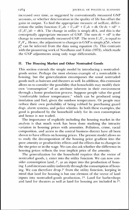