Embed Size (px)
Citation preview

2 Trade and Technology: The Ricardian Model 1. In this problem you will use the World Development Indicators (WDI) database from the
World Bank to compute the comparative advantage of two countries in the major sectors of gross domestic product (GDP): agriculture, industry (which includes manufacturing, mining, construction, electricity, and gas), and services. Go to the WDI website at http://wdi.worldbank.org, and choose “Online tables,” where you will be using the sections on “People” and on the “Economy.”
a. In the “People” section, start with the table “Labor force structure.” Choose two countries that you would like to compare, and for a recent year write down their total labor force (in millions) and the percentage of the labor force that is female. Then calculate the number of the labor force (in millions) who are male and the number who are female.
Answer:
2014
Labor Force
(million)
Female Labor
(%)
Male Labor
(million)
Female Labor
(million)
France
30.1
47
15.95
14.15
Thailand
40.1
46
18.45
21.65
b. Again using the “People” section of the WDI, now go to the “Employment by sector” table. For the same two countries that you chose in part (a) and for roughly the same year, write down the percent of male employment and the percent of female employment in each of the three sectors of GDP: agriculture, industry, and services. (If the data are missing in this table for the countries that you chose in part (a), use different countries.) Use these percentages along with your answer to part (a) to calculate the number of male workers and the number of female workers in each sector. Add together the number of male and female workers to get the total labor force in each sector.
Answer:
2011–2014
Agriculture
Male % Female %
Industry
Male % Female %
Service
Male % Female %
France
4
2
31
10
65
88
Thailand
44
39
23
18
33
43
International Economics 4th Edition Feenstra Solutions ManualFull Download: https://testbanklive.com/download/international-economics-4th-edition-feenstra-solutions-manual/
Full download all chapters instantly please go to Solutions Manual, Test Bank site: testbanklive.com

2011–2014 (million)
Agriculture
Male Female
Industry
Male Female
Service
Male Female
France
0.64
0.28
4.95
1.42
10.37
12.45
Thailand
8.12
8.44
4.24
3.90
6.09
9.31
c. In the “Economy” section, go to the table “Structure of output.” There you will find GDP (in $ billions) and the % of GDP in each of the three sectors: agriculture, industry, and services. For the same two countries and the same year that you chose in part (a), write down their GDP (in $ billions) and the percentage of their GDP accounted for by agriculture, by industry, and by services. Multiply GDP by the percentages to obtain the dollar amount of GDP coming from each of these sectors, which is interpreted as the value-added in each sector, that is, the dollar amount that is sold in each sector minus the cost of materials (not including the cost of labor or capital) used in production.
Answer:
2014
GDP (billion $)
Agriculture (%)
Industry (%)
Service (%)
France
2829.2 2
19
79
Thailand
404.8
20
37
53
d. Using your results from parts (b) and (c), divide the GDP from each sector by the labor force in each sector to obtain the value-added per worker in each sector. Arrange these numbers in the same way as the “Sales/Employee” and “Bushels/Worker” shown in Table 2-2. Then compute the absolute advantage of one country relative to the other in each sector, as shown on the right-hand side of Table 2-2. Interpret your results. Also compute the comparative advantage of agriculture/industry and agriculture/services (as shown at the bottom of Table 2-2), and the comparative advantage of industry/services. Based on your results, what should be the trade pattern of these two countries if they were trading only with each other?

Answer:
($1000)
France
Thailand Absolute Advantage France/Thailand Ratio
Service
97.94
13.93
7.03
Industry
84.39
18.4
4.59
Agriculture
61.50
4.89
12.58
Comparative Advantage
Agriculture/ Service
0.63
0.35
Agriculture/ Industry
0.73
0.27
Industry/Service
0.86
1.33
Thailand has a comparative advantage in both Service and Industry. Suppose that a farmer spends 1,000 hours per year in agriculture production. Multiplying the marginal product of an hour of labor in agriculture by 1,000, to obtain the marginal production of labor per year and dividing by the marginal production of labor in Service gives us the opportunity cost of Service. In France, this ratio is 0.63, indicating that $0.63 must be foregone to obtain an extra dollar of sales in Agriculture. In Industry, the ratio is 0.73 in France. These ratios are much smaller in Thailand, only 0.35 for Service and 0.27 for Industry. As a result, Thailand has a lower opportunity cost of both Industry and Service. Therefore, if assuming the two countries are trading only with each other, France will export Agriculture while Thailand will export Service and Industry.
2. At the beginning of the chapter, there is a brief quotation from David Ricardo; here is a longer version of what Ricardo wrote:
England may be so circumstanced, that to produce the cloth may require the labour of 100 men for one year; and if she attempted to make the wine, it might require the labour of 120 men for the same time. . . . To produce the wine in Portugal, might require only the labour of 80 men for one year, and to produce the cloth in the same country, might require the labour of 90 men for the same time. It would therefore be advantageous for her to export wine in exchange for cloth. This exchange might even take

place, notwithstanding that the commodity imported by Portugal could be produced there with less labour than in England.
Suppose that the amount of labor Ricardo describes can produce 1,000 yards of cloth or 2,000 bottles of wine in either country. Then answer the following:
a. What is England’s marginal product of labor in cloth and in wine, and
what is Portugal’s marginal product of labor in cloth and in wine? Which country has absolute advantage in cloth, and in wine, and why? Answer: In England, 100 men produce 1,000 yards of cloth, so MPLC = 1,000/100 = 10. 120 men produce 2,000 bottles of wine, so MPLW = 2,000/120 =16.6. In Portugal, 90 men produce 1,000 yards of cloth, so MPL*
C = 1,000/90 = 11.1. Eighty (80) men produce 2,000 bottles of wine, so MPL*
w = 2,000/80 = 25. So Portugal has an absolute advantage in both cloth and wine, because it has higher marginal products of labor in both industries than does England.
b. Use the formula PW/PC = MPLC/MPLW to compute the no-trade relative price of wine
in each country. Which country has comparative advantage in wine, and why? Answer: For England, PW/PC = MPLC/MPLW = 10/16.6 = 0.6, which is the no-trade relative price of wine (equal to the opportunity cost of producing wine). So the opportunity cost of wine in terms of cloth is 0.6, meaning that to produce 1 bottle of wine in England, the country gives up 0.6 yards of cloth. For Portugal, PW
*/PC*=
MPLC*/MPLW
* = 11.1/25 = 0.4, which is the no-trade relative price of wine (equal to the opportunity cost of producing wine). The no-trade relative price of wine is lower in Portugal, so Portugal has comparative advantage in wine, and England has comparative advantage in cloth. Portugal has comparative advantage in producing wine because it has lower opportunity cost (PW
*/PC*= 0.4) than England in the
production of wine (PW/PC = 0.6).

3. Suppose that each worker in Home can produce two cars or three TVs. Assume that
Home has four workers. a. Graph the production possibilities frontier for Home. Answer: See the following figure.
b. What is the no-trade relative price of cars in Home? Answer: The no-trade relative price of cars at Home is PC/PTV = 3/2 =
MPLTV/MPC. It is the slope of the PPF curve for Home. 4. Suppose that each worker in Foreign can produce three cars or two TVs. Assume that
Foreign also has four workers. a. Graph the production possibilities frontier for Foreign. Answer: See following figure.

b. What is the no-trade relative price of cars in Foreign? Answer: The no-trade relative price of cars in Foreign is P*
C/P*TV = 2/3 =
c. Using the information provided in Problem 3 regarding Home, in which good does
Foreign have a comparative advantage, and why? Answer: Foreign has a comparative advantage in producing televisions because it
has a lower opportunity cost than Home in the production of televisions. 5. Suppose that in the absence of trade, Home consumes two cars and nine TVs, while
Foreign consumes nine cars and two TVs. Add the indifference curve for each country to the figures in Problems 3 and 4. Label the production possibilities frontier (PPF), indifference curve (U1), and the no-trade equilibrium consumption and production for each country.
Answer: See following figures.

6. Now suppose the world relative price of cars is PC/PTV = 1. a. In what good will each country specialize? Briefly explain why. Answer: Home would specialize in TVs, export TVs, and import cars, whereas
the Foreign country would specialize in cars, export cars, and import TVs. The reason is because Home has a comparative advantage in TVs and Foreign has a comparative advantage in cars.
b. Graph the new world price line for each country in the figures in Problem 5, and
add a new indifference curve (U2) for each country in the trade equilibrium. Answer: See the following figures.
c. Label the exports and imports for each country. How does the amount of Home

exports compare with Foreign imports? Answer: See graph in part (b). The amount of Home TV exports is equal to the
amount of Foreign TV imports. In addition, Home imports of cars equal Foreign exports of cars. This is balanced trade, which is an essential feature of the Ricardian model.
d. Does each country gain from trade? Briefly explain why or why not. Answer: Both Home and Foreign benefit from trade relative to their no-trade
consumption because their utilities are both higher (consumption bundles located on higher indifference curves).
Work It Out Answer the following questions using the information given by the accompanying
table.
Home Foreign Absolute Advantage Number of bicycles produced per hour
4 6 ?
Number of snowboards produced per hour
6 8 ?
Comparative Advantage ? ?
a. Complete the table for this problem in the same manner as Table 2-2. Answer: See previous table. b. Which country has an absolute advantage in the production of bicycles? Which
country has an absolute advantage in the production of snowboards? Answer: Foreign has an absolute advantage in both production of bicycles and
snowboards, because it is able to produce more in an hour than Home. c. What is the opportunity cost of bicycles in terms of snowboards in Home? What
is the opportunity cost of bicycles in terms of snowboards in Foreign? Answer: The opportunity cost of one bicycle is 3/2 snowboards at Home (PB/PS =
MPLS/MPLB = 6/4 = 3/2). The opportunity cost of one bicycle is 4/3 snowboards in the Foreign country (PB
*/PS* = MPLS
*/MPLB* = 8/6 = 4/3).
d. Which product will Home export, and which product does Foreign export? Briefly explain why.
Answer: The opportunity cost of one bicycle is 3/2 snowboards at Home (PB/PS = MPLS/MPLB = 6/4 = 3/2). The opportunity cost of one bicycle is 4/3 snowboards in the Foreign country (PB
*/PS* = MPLS
*/MPLB* = 8/6 = 4/3). Home has a smaller
opportunity cost producing snowboards than the Foreign country. Home will export snowboards and Foreign will export bicycles.

7. Assume that Home and Foreign produce two goods, TVs and cars, and use the
information below to answer the following questions: In the No-Trade equilibrium:
Home Foreign WageTV = 12 WageC = ? Wage*
TV = ? Wage*C = 6
MPLTV = 4 MPLC = ? MPL*TV = ? MPL*
C = 1
PTV = ? PC = 4 P*TV = 8 P*
C = ? a. What is the marginal product of labor for TVs and cars in Home? What is the no-
trade relative price of TVs in Home? Answer: MPLC = 3, MPLTV = 4, and PTV/PC = MPLC /MPLTV = 3/4 b. What is the marginal product of labor for TVs and cars in Foreign? What is the
no-trade relative price of TVs in Foreign? Answer: MPL*
C = 1, MPL*TV = 3/4, and P*
TV/P*C = MPL*
C/MPL*TV = 4/3
c. Suppose the world relative price of TVs in the trade equilibrium is PTV/PC = 1.
Which good will each country export? Briefly explain why. Answer: Home will export TVs and Foreign will export cars because Home has a comparative advantage in TVs whereas Foreign has a comparative advantage in car. Each country will specialize in the goods with lower opportunity cost.
d. In the trade equilibrium, what is the real wage in Home in terms of cars and in
terms of TVs? How do these values compare with the real wage in terms of either good in the no-trade equilibrium?
Answer: Workers at Home are paid in terms of TVs because Home exports TVs. Home is better off with trade because its real wage in terms of cars has increased.
MPLTV = 4 units of TVHome wages with trade= or (PTV /PC ) ⋅MPLTV = (1) ⋅ =4 4 units of car
MPLTV = 4 units of TVHome wages w/o trade= or (PTV /PC ) ⋅MPLTV = (3/4) ⋅ =4 3 units of car

e. In the trade equilibrium, what is the real wage in Foreign in terms of TVs and in
terms of cars? How do these values compare with the real wage in terms of either good in the no-trade equilibrium?
Answer: Foreign workers are paid in terms of cars because Foreign exports cars. Foreign gains in terms of cars with trade.
(P /P ) ⋅MPL*
C TV C = (1) ⋅ =1 1 units of TVForeign wages with trade= or = MPL*
C 1 units of car
(P* */P ) ⋅MPL*C TV C = (3/4) ⋅ =1 3/4 unit of TV
Foreign wages w/o trade= or MPL*
C = 1 units of car f. In the trade equilibrium, do Foreign’s workers earn more or less than Home’s
workers, measured in terms of their ability to purchase goods? Explain why. Answer: Foreign workers earn less than workers at Home in terms of cars
because Home has an absolute advantage in the production of cars. Home workers also earn more than Foreign workers in terms of TVs
8. Why do some low-wage countries, such as China, pose a threat to manufacturers in
industrial countries, such as the United States, whereas other low-wage countries, such as Haiti, do not?
Answer: To engage in international trade, a country must have a minimal threshold of productivity. Countries such as China have the productivity necessary to compete successfully, but Haiti does not. China can enter the world market because it beats other industrial countries with a lower price. Under perfect competition, price is determined by both wage rate and productivity; that is, P = Wage/MPL. So the lower price in China comes from both a low wage rate and high MPL. Haiti has a low wage rate, but also low MPL. So Haiti’s price is not low enough to enter the world market.
Answer Problems 9 to 11 using the chapter information for Home and Foreign. 9. a. Suppose that the number of workers doubles in Home. What happens to the Home
PPF and what happens to the no-trade relative price of wheat?

Answer: With the doubling of the number of workers in Home, it can now
produce 200 = 4 · 50 bushels of wheat if it concentrates all resources in the production of wheat, or it could produce 100 = 2 · 50 yards of cloth by devoting all resources to the production of cloth. The PPF shifts out for both wheat and cloth. The no-trade relative price of wheat remains the same because both MPLW and MPLC are unchanged.
b. Suppose that there is technological progress in the wheat industry such that Home
can produce more wheat with the same amount of labor. What happens to the Home PPF and what happens to the relative price of wheat? Describe what would happen if a similar change occurred in the cloth industry.

Answer: Because the technological progress is only in the wheat industry,
Home’s production of cloth remains the same if it devotes all of its resources to producing cloth. If instead Home produces only wheat, it is able to produce more wheat using the same amount of labor. Home’s PPF shifts out in the direction of wheat production. Recall that the relative price of wheat is given by PW/PC = MPLC/MPLW. With the technological progress in wheat, the marginal product of labor in the wheat production increases. Thus, the relative price of wheat decreases. As shown in the graph, the relative price of wheat drops from 1/2 to 1/4.
If instead the technological progress is in the cloth industry, we would have the opposite results. Home’s PPF would shift out in the direction of cloth production and the relative price of wheat would increase.
10. a. Using Figure 2-5, show that an increase in the relative price of wheat from its
world relative price of 23 will raise Home’s utility.

Answer: The increase in the relative price of wheat from its international
equilibrium of 2/3 allows Home to consume at a higher utility, such as at point D. b. Using Figure 2-6, show that an increase in the relative price of wheat from its
world relative price of 23will lower Foreign’s utility. What is Foreign’s utility
when the world relative price reaches 1, and what happens in Foreign when the world relative price of wheat rises above that level?
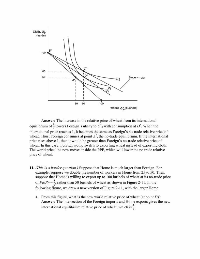
Answer: The increase in the relative price of wheat from its international equilibrium of 2
3 lowers Foreign’s utility to U*
3 with consumption at D*. When the international price reaches 1, it becomes the same as Foreign’s no-trade relative price of wheat. Thus, Foreign consumes at point A*, the no-trade equilibrium. If the international price rises above 1, then it would be greater than Foreign’s no-trade relative price of wheat. In this case, Foreign would switch to exporting wheat instead of exporting cloth. The world price line now moves inside the PPF, which will lower the no trade relative price of wheat. 11. (This is a harder question.) Suppose that Home is much larger than Foreign. For
example, suppose we double the number of workers in Home from 25 to 50. Then, suppose that Home is willing to export up to 100 bushels of wheat at its no-trade price of PW/PC = 1
2, rather than 50 bushels of wheat as shown in Figure 2-11. In the
following figure, we draw a new version of Figure 2-11, with the larger Home. a. From this figure, what is the new world relative price of wheat (at point D)? Answer: The intersection of the Foreign imports and Home exports gives the new
international equilibrium relative price of wheat, which is 12.

b. Using this new world equilibrium price, draw a new version of the trade
equilibrium in Home and in Foreign, and show the production point and consumption point in each country.
Answer: The international price of 12 is the same as Home’s no-trade relative price
of wheat. Home would consume at point A and produce at point B´. The difference between these two points gives Home exports of wheat of 80 units. (Notice that workers earn equal wages in the two industries, so production can occur anywhere along the PPF.)

Because the international price of 1/2 is lower than Foreign’s no-trade relative
price of wheat, Foreign is able to consume at point D*, which gives higher gains from trade than at point C*.

c. Are there gains from trade in both countries? Explain why or why not. Answer: The Foreign country gains a lot from trade, but the home country neither
gains nor loses: Its consumption point A is exactly the same as what it would be in the absence of trade. This shows that in the Ricardian model, a small country can gain the most from trade, whereas a large country may not gain (although it will not lose) because the world relative price might equal its own no-trade relative price. So the large country does not see a terms of trade (TOT) gain. This special result will not arise in other models that we study, but illustrates how being small can help a country on world markets!
12. Using the results from Problem 11, explain why the Ricardian model predicts that
Mexico would gain more than the United States when the two countries signed the North American Free Trade Agreement, establishing free trade between them.
Answer: The Ricardian model predicts that Mexico would gain more than the United States when the two countries join the regional trade agreement because relative to the United States in terms of economic size, Mexico is a small country. For the United States, the world price of its exports is similar to the domestic price. Thus, there is not much TOT gain. But for Mexico, the world price is much higher than the domestic price of its exports, so Mexico sees a big TOT improvement.

2 (13) Introduction to Exchange Rates and the Foreign Exchange Market 1. Discovering Data Not all pegs are created equal! In this question you will explore trends in exchange rates. Go to the St. Louis Federal Reserve’s Economic Data (FRED) website at https://research.stlouisfed.org/fred2/ and download the daily United States exchange rates with Venezuela, India, and Hong Kong from 1990 to present. These can be found most easily by searching for the country names and “daily exchange rate.”
a. Plot the Indian rupee to U.S. dollar exchange rate over this period. For what years does the rupee appear to be pegged to the dollar? Does this peg break? If so, how many times? Answer: The rupee appears to be pegged to the U.S. dollar at various rates from 1991 until about 1998 with intermittent volatility at places the peg appears to break. There are four distinct rates at which this peg remains, the longest of which lasting over two years from 1993 until mid 1995.
b. How would you characterize the relationship between the rupee and the dollar from 1998–2008? Does it appear to be fixed, crawling, or floating during this period? How would you characterize it from 2008 onward? Answer: Over this period the exchange rate appears to be a crawling peg. Although this crawl is relatively flat for a few years at the beginning of this period, it appears free to move. However, the lack of short-term volatility suggests that the exchange rate is still being controlled and is hence crawling. From 2008 onward this appears to be a freely floating currency. The line becomes more erratic with a greater deal of short-term volatility. c. The Hong Kong dollar has maintained its peg with the United States dollar since 1983. Over the course of the period that you have downloaded what are the highest and lowest values for this exchange rate?
0.0000
10.0000
20.0000
30.0000
40.0000
50.0000
60.0000
70.0000
80.0000
1990
-01-
0219
91-0
1-02
1992
-01-
0219
93-0
1-02
1994
-01-
0219
95-0
1-02
1996
-01-
0219
97-0
1-02
1998
-01-
0219
99-0
1-02
2000
-01-
0220
01-0
1-02
2002
-01-
0220
03-0
1-02
2004
-01-
0220
05-0
1-02
2006
-01-
0220
07-0
1-02
2008
-01-
0220
09-0
1-02
2010
-01-
0220
11-0
1-02
2012
-01-
0220
13-0
1-02
2014
-01-
0220
15-0
1-02
2016
-01-
02
Rupee/Dollar Exchange Rate

Answer: This peg has never broken over this period (although there is some movement if you allow the axis to be small enough). The highest rate that it has attained is 7.8289 Hong Kong dollars per US dollar on August 6, 2007, at the height of the financial crisis. The lowest it has gone is 7.7085 on October 6, 2003.
d. Venezuela has been less successful in its attempts to fix against the dollar. Since 1995 how many times has the Venezuelan bolívar peg to the dollar broken? What is the average length of a peg? What is the average size of a devaluation? Answer: I count seven breaks in this peg over this period. In 1998 they appear to move to a slow and managed crawl before floating for a short time and returning to a fixed rate. The longest period of any one peg appears to be when the exchange rate was set at 2.14 bolívar/dollar for about five years between 2005 and 2010.
7.0000
7.2000
7.4000
7.6000
7.8000
8.0000
8.2000
8.4000
8.6000
8.8000
9.000019
90-0
1-02
1991
-01-
0219
92-0
1-02
1993
-01-
0219
94-0
1-02
1995
-01-
0219
96-0
1-02
1997
-01-
0219
98-0
1-02
1999
-01-
0220
00-0
1-02
2001
-01-
0220
02-0
1-02
2003
-01-
0220
04-0
1-02
2005
-01-
0220
06-0
1-02
2007
-01-
0220
08-0
1-02
2009
-01-
0220
10-0
1-02
2011
-01-
0220
12-0
1-02
2013
-01-
0220
14-0
1-02
2015
-01-
0220
16-0
1-02
Hong Kong/US Exchange Rate

2. Refer to the exchange rates given in the following table:
January 20, 2016 January 20, 2015 Country (currency) FX per $ FX per £ FX per € FX per $ Australia (dollar) 1.459 2.067 1.414 1.223 Canada (dollar) 1.451 2.056 1.398 1.209 Denmark (krone) 6.844 9.694 7.434 6.430 Eurozone (euro) 0.917 1.299 1.000 0.865 Hong Kong (dollar) 7.827 11.086 8.962 7.752 India (rupee) 68.05 96.39 71.60 61.64 Japan (yen) 116.38 164.84 136.97 118.48 Mexico (peso) 18.60 26.346 16.933 14.647 Sweden (krona) 8.583 12.157 9.458 8.181 United Kingdom (pound) 0.706 1.000 0.763 0.600 United States (dollar) 1.000 1.416 1.156 1.000
Data from: U.S. Federal Reserve Board of Governors, H.10 release: Foreign Exchange Rates. Based on the table provided, answer the following questions: a. Compute the U.S. dollar–yen exchange rate E$/¥ and the U.S. dollar–Canadian
dollar exchange rate E$/C$ on January 20, 2016, and January 20, 2015. Answer: U.S. dollar–yen rates: January 20, 2015: E$/¥ = 1/(118.48) = $0.0084/¥ January 20, 2016: E$/¥ = 1/(116.38) = $0.0086/¥ January 20, 2015: E$/C$ = 1/(1.209) = $0.8271/C$ January 20, 2016: E$/C$ = 1/(1.451) = $0.6892/C$
0
2
4
6
8
10
12
Venezuela/US Exchange Rate
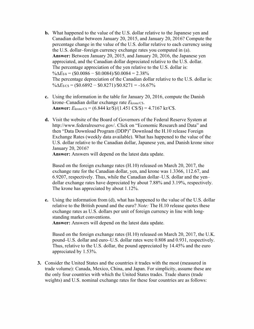
b. What happened to the value of the U.S. dollar relative to the Japanese yen and Canadian dollar between January 20, 2015, and January 20, 2016? Compute the percentage change in the value of the U.S. dollar relative to each currency using the U.S. dollar–foreign currency exchange rates you computed in (a).
Answer: Between January 20, 2015, and January 20, 2016, the Japanese yen appreciated, and the Canadian dollar depreciated relative to the U.S. dollar.
The percentage appreciation of the yen relative to the U.S. dollar is: %∆E$/¥ = ($0.0086 − $0.0084)/$0.0084 = 2.38% The percentage depreciation of the Canadian dollar relative to the U.S. dollar is: %∆E$/C$ = ($0.6892 − $0.8271)/$0.8271 = -16.67% c. Using the information in the table for January 20, 2016, compute the Danish
krone–Canadian dollar exchange rate Ekrone/C$. Answer: Ekrone/C$ = (6.844 kr/$)/(1.451 C$/$) = 4.7167 kr/C$. d. Visit the website of the Board of Governors of the Federal Reserve System at
http://www.federalreserve.gov/. Click on “Economic Research and Data” and then “Data Download Program (DDP)” Download the H.10 release Foreign Exchange Rates (weekly data available). What has happened to the value of the U.S. dollar relative to the Canadian dollar, Japanese yen, and Danish krone since January 20, 2016?
Answer: Answers will depend on the latest data update. Based on the foreign exchange rates (H.10) released on March 20, 2017, the
exchange rate for the Canadian dollar, yen, and krone was 1.3366, 112.67, and 6.9207, respectively. Thus, while the Canadian dollar–U.S. dollar and the yen–dollar exchange rates have depreciated by about 7.88% and 3.19%, respectively. The krone has appreciated by about 1.12%.
e. Using the information from (d), what has happened to the value of the U.S. dollar
relative to the British pound and the euro? Note: The H.10 release quotes these exchange rates as U.S. dollars per unit of foreign currency in line with long-standing market conventions.
Answer: Answers will depend on the latest data update. Based on the foreign exchange rates (H.10) released on March 20, 2017, the U.K.
pound–U.S. dollar and euro–U.S. dollar rates were 0.808 and 0.931, respectively. Thus, relative to the U.S. dollar, the pound appreciated by 14.45% and the euro appreciated by 1.53%.
3. Consider the United States and the countries it trades with the most (measured in
trade volume): Canada, Mexico, China, and Japan. For simplicity, assume these are the only four countries with which the United States trades. Trade shares (trade weights) and U.S. nominal exchange rates for these four countries are as follows:

Country (currency) Share of Trade $ per FX in 2015 $ per FX in 2016 Canada (dollar) 36% 0.8271 0.6892 Mexico (peso) 28% 0.0683 0.0538 China (yuan) 20% 0.1608 0.1522 Japan (yen) 16% 0.0080 0.0086
a. Compute the percentage change from 2015 to 2016 in the four U.S. bilateral
exchange rates (defined as U.S. dollars per unit of foreign exchange, or FX) in the table provided.
Answer: %∆E$/C$ = (0.6892 − 0.8271)/0.8271 = −16.67% %∆E$/pesos = (0.0538 − 0.0683)/0.0683 = −21.23% %∆E$/yuan = (0.1522 − 0.1608)/0.1608 = −5.35% %∆E$/¥ = (0.0086 − 0.008/0.008 = 7.50% b. Use the trade shares as weights to compute the percentage change in the nominal
effective exchange rate for the United States between 2015 and 2016 (in U.S. dollars per foreign currency basket).
Answer: The trade-weighted percentage change in the exchange rate is: %∆E = 0.36(%∆E$/C$) + 0.28(%∆E$/pesos) + 0.20(%∆E$/yuan) + 0.16(%∆E$/¥) %∆E = 0.36(−16.67 %) + 0.28(−21.23%) + 0.20(−5.35%) + 0.16(7.50%) = −11.82% c. Based on your answer to (b), what happened to the value of the U.S. dollar against
this basket between 2015 and 2016? How does this compare with the change in the value of the U.S. dollar relative to the Mexican peso? Explain your answer.
Answer: The dollar appreciated by 11.82% against the basket of currencies. Vis-à-vis the peso, the dollar appreciated by 21.23%. The average depreciation is smaller because the dollar depreciated by only 5.35% against China with a 20% trade share and appreciated against the yen with a 16% trade share.
4. Go to the FRED website: http://research.stlouisfed.org/fred2/. Locate the monthly
exchange rate data for the following: Look at the graphs and make your own judgment as to whether each currency was
fixed (peg or band), crawling (peg or band), or floating relative to the U.S. dollar during each time frame given.
a. Canada (dollar), 1980–2012 Answer: Floating exchange rate b. China (yuan), 1999–2004, 2005–09, and 2009–10 Answer: 1999–2004: fixed exchange rate; 2005–09: gradual appreciation vis-à-
vis the dollar; again fixed for 2009–10 c. Mexico (peso), 1993–95 and 1995–2012 Answer: 1993–95: crawl; 1995–2012: floating (with some evidence of a managed

float) d. Thailand (baht), 1986–97 and 1997–2012 Answer: 1986–97: fixed exchange rate; 1997–2012: floating e. Venezuela (bolívar), 2003–12 Answer: fixed exchange rate (with occasional adjustments) 5. Describe the different ways in which the government may intervene in the forex
market. Why does the government have the ability to intervene in this way, while private actors do not?
Answer: The government may participate in the forex market in a number of ways: capital controls, establishing an official market (with fixed rates) for forex transactions, and forex intervention by buying and selling currencies in the forex markets. The government has the ability to intervene in a way that private actors do not because through its central bank it has unlimited stock of its own currency and usually a large stock of foreign reserves. Its intervention is guided by policy rather than merely making profits on currency trade, which is the case with the private sector.
Work it out. Consider a Dutch investor with 1,000 euros to place in a bank deposit in
either the Netherlands or Great Britain. The (one-year) interest rate on bank deposits is 1% in Britain and 5% in the Netherlands. The (one-year) forward euro–pound exchange rate is 1.65 euros per pound and the spot rate is 1.5 euros per pound. Answer the following questions, using the exact equations for uncovered interest parity (UIP) and covered interest parity (CIP) as necessary.
a. What is the euro-denominated return on Dutch deposits for this investor? Answer: The investor’s return on euro-denominated Dutch deposits is equal to
€1,050 = €1,000 × (1 + 0.05). b. What is the (riskless) euro-denominated return on British deposits for this investor
using forward cover? Answer: The euro-denominated return on British deposits using forward cover is
equal to €1,111 (= €1,000 × (1.65/1.5) × (1 + 0.01)). c. Is there an arbitrage opportunity here? Explain why or why not. Is this an
equilibrium in the forward exchange rate market? Answer: Yes, there is an arbitrage opportunity. The euro-denominated return on
British deposits is higher than that on Dutch deposits. The net return on each euro deposit in a Dutch bank is equal to 5% versus 11.1% (= (1.65/1.5) × (1 + 0.01)) on a British deposit (using forward cover). This is not an equilibrium in the forward exchange market. The actions of traders seeking to exploit the arbitrage opportunity will cause the spot and forward rates to change.

d. If the spot rate is 1.5 euros per pound, and interest rates are as stated previously, what is the equilibrium forward rate, according to CIP?
Answer: CIP implies F€/£ = E€/£ (1 + i€)/(1 + i£) = 1.65 × 1.05/1.01 = €1.72 per £. e. Suppose the forward rate takes the value given by your answer to (d). Compute
the forward premium on the British pound for the Dutch investor (where exchange rates are in euros per pound). Is it positive or negative? Why do investors require this premium/discount in equilibrium?
Answer: Forward premium = (F€/£/E€/£ − 1) = (1.72/1.50) − 1 = 0.1467 or 14.67%. The existence of a positive forward premium would imply that investors expect the euro to depreciate relative to the British pound. Therefore, when establishing forward contracts, the forward rate is higher than the current spot rate.
f. If UIP holds, what is the expected depreciation of the euro (against the pound)
over one year? Answer: If UIP holds, the expected euro–pound exchange rate is the same as the
forward rate, that is, € 1.72 per £ (see part (d) above). The expected depreciation of Euro against pound is therefore 14.67%.
g. Based on your answer to (f), what is the expected euro–pound exchange rate one
year ahead? Answer: Following the answer to parts (d) and (f), the expected euro–pound
exchange rate is €1.72 per £ or 1/1.72 = 0.5814 £/€. 6. Suppose quotes for the dollar–euro exchange rate E$/€ are as follows: in New York
$1.05 per euro, and in Tokyo $1.15 per euro. Describe how investors use arbitrage to take advantage of the difference in exchange rates. Explain how this process will affect the dollar price of the euro in New York and Tokyo.
Answer: Investors will buy euros in New York at a price of $1.05 each because this is relatively cheaper than the price in Tokyo. They will then sell these euros in Tokyo at a price of $1.15, earning a $0.10 profit on each euro. With the influx of buyers in New York, the price of euros in New York will increase. With the influx of traders selling euros in Tokyo, the price of euros in Tokyo will decrease. This price adjustment continues until the exchange rates are equal in both markets.
7. You are a financial adviser to a U.S. corporation that expects to receive a payment of
60 million Japanese yen in 180 days for goods exported to Japan. The current spot rate is 100 yen per U.S. dollar (E$/¥ = 0.01000). You are concerned that the U.S. dollar is going to appreciate against the yen over the next six months.
a. Assuming the exchange rate remains unchanged, how much does your firm expect
to receive in U.S. dollars? Answer: The firm expects to receive $600,000 (= ¥60,000,000/100).

b. How much would your firm receive (in U.S. dollars) if the dollar appreciated to
110 yen per U.S. dollar (E$/¥ = 0.00909)? Answer: The firm would receive $545,454 (= ¥60,000,000/110). c. Describe how you could use an options contract to hedge against the risk of losses
associated with the potential appreciation in the U.S. dollar. Answer: The firm could buy ¥60 million in call options on dollars, say, for
example, at a rate of 105¥ per dollar. A call option gives the buyer a right to buy dollars at the price agreed upon. If the dollar appreciates such that its price rises above 105¥, say to 110¥, the firm will exercise the option. This ensures the firm’s yen receipts will at least be worth $571,428 (= ¥60,000,000/105).
8. Consider how transactions costs affect foreign currency exchange. Rank each of the
following foreign exchanges according to their probable spread (between the “buy at” and “sell for” bilateral exchange rates) and justify your ranking.
a. An American returning from a trip to Turkey wants to exchange his Turkish lira
for U.S. dollars at the airport. b. Citigroup and HSBC, both large commercial banks located in the United States
and United Kingdom, respectively, need to clear several large checks drawn on accounts held by each bank.
c. Honda Motor Company needs to exchange yen for U.S. dollars to pay American workers at its Ohio manufacturing plant.
d. A Canadian tourist in Germany pays for her hotel room using a credit card. Answer: Ranking (highest spread first): (a), (d), (c), (b). Both (a) and (d) involve
small transactions that will involve a go-between who will charge a premium to convert the currency. (d) involves a credit card company (a commercial bank or nonbank financial institution) that likely is involved in large volumes of transactions each day. (c) involves a corporation that can negotiate a better rate (versus an individual) because it will likely engage in a large currency exchange, or Honda could simply enter the market without going through a broker. Finally, (b) involves two large commercial banks that regularly engage in large-volume foreign exchange trading.

13 Introduction to Exchange Rates and the Foreign Exchange Market
Notes to the Instructor
Chapter Summary This chapter introduces students to exchange rates, to the foreign exchange (forex)
market, to the way foreign currency is exchanged in private and government transactions,
and to arbitrage conditions in the forex market. The chapter begins with a discussion of
the ways exchange rates affect international trade and asset transactions. After covering
the basics, the chapter covers foreign exchange markets, spot exchange rates, interest
rates, and arbitrage in both spot and asset markets.
Comments Although most students have heard of exchange rates (either in the media or in previous
economics classes), few will understand how the foreign exchange market works and
how arbitrage is important in financial markets. This chapter serves two functions: (1) to
provide information on how the foreign exchange market works in practice (Sections 1
through 3), and (2) to establish a foundation for model-building in subsequent chapters
(Sections 4 and 5).
The chapter contains a large amount of detailed information. Because much of it is
fundamental in the development of concepts and models throughout the text, it is worth
spending more time on this material than might otherwise be devoted to a typical
textbook chapter. There are optional advanced topics and case studies that the instructor
may elect to skip without compromising material in later chapters.

An outline of the chapter follows.
1. Exchange Rate Essentials
a. Defining the Exchange Rate
b. Appreciations and Depreciations
c. Multilateral Exchange Rates
d. Example: Using Exchange Rates to Compare Prices in a Common Currency
i. Scenario 1
ii. Scenario 2
iii. Scenario 3
iv. Scenario 4
v. Generalizing
2. Exchange Rates in Practice
a. Exchange Rate Regimes: Fixed Versus Floating
b. Application: Recent Exchange Rate Experiences
i. Evidence from Developed Countries
ii. Evidence from Developing Countries
iii. Currency Unions and Dollarization
iv. Exchange Rate Regimes of the World
v. Looking Ahead
3. The Market for Foreign Exchange
a. The Spot Contract
b. Transaction Costs
c. Derivatives
d. Application: Foreign Exchange Derivatives
i. Forwards
ii. Swaps
iii. Futures
iv. Options
e. Private Actors
f. Government Actions
4. Arbitrage and Spot Exchange Rates
a. Arbitrage with Two Currencies
b. Arbitrage with Three Currencies
c. Cross Rates and Vehicle Currencies
5. Arbitrage and Interest Rates
i. The Problem of Risk
a. Riskless Arbitrage: Covered Interest Parity
i. What Determines the Forward Rate?
b. Application: Evidence on Covered Interest Parity
c. Risky Arbitrage: Uncovered Interest Parity
i. Side Bar: Assets and Their Attributes
ii. What Determines the Spot Rate?
d. Application: Evidence on Uncovered Interest Parity
e. Uncovered Interest Parity: A Useful Approximation
6. Conclusions

Lecture Notes
The exchange rate affects both the price Americans pay for foreign goods and services
and the price foreigners pay for U.S. goods and services. The exchange rate also affects
the cost of investment across countries. For these reasons, policy makers are concerned
with the value of the domestic currency relative to the rest of the world. Before
examining how the exchange rate fits into the economy, this chapter begins with defining
the exchange rate and then describes the market for foreign exchange.
1 Exchange Rate Essentials
An exchange rate (E) is the price of a foreign currency expressed in terms of a home
currency. Because an exchange rate is the relative price of two currencies, it may be
quoted in either of two ways:
1. The number of home currency units that can be exchanged for one unit of foreign
currency. For example, if the United States is considered home, the dollar/euro
exchange rate might be $1.15 per euro (or 1.15 $/€). To buy one euro, you would
have to pay $1.15.
2. The number of foreign currency units that can be exchanged for one unit of home
currency. For example, the $1.15/€ exchange rate can also be expressed as €0.87
per U.S. dollar (or 0.87 €/$). To buy one dollar, you would have to pay €0.87.
The examples in this section of the Instructor's Manual parallel those in the text but
use different currencies and exchange rates. In all cases, the United States is the home
country. These examples are for instructors who don’t want their lecture to explain only
what’s in the textbook.

Defining the Exchange Rate By convention, the exchange rate is defined as units of domestic currency per unit of
foreign currency. Thus, E1/2 is the number of units of country 1’s currency needed to buy
one unit of country 2’s currency.
Consider two countries: the United States and the United Kingdom. These regions use
the U.S. dollar ($) and the British pound (£), respectively.
The exchange rate above implies an American must pay $1.80 for each British pound.
We can use this exchange rate to determine how much a U.K. resident would pay for a
U.S. dollar:
𝐸𝐸£/$ = 1𝐸𝐸£/$
= 11.80
= 0.56
This means a British resident must pay 0.56 British pounds to buy one U.S. dollar.
Appreciations and Depreciations Appreciation and depreciation are terms used to describe how the value of a currency
changes over time. Because we’ve defined the exchange rate as a bilateral exchange rate,

an increase in the value of one currency (appreciation) implies a decrease in the value of
the other currency (depreciation). For example, if the dollar–pound exchange rate falls
from E$/£ = 1.80 to E$/£ = 1.60, Americans must pay fewer U.S. dollars for the same
British pound. Since it takes fewer dollars to buy one pound, the dollar has appreciated
vis-à-vis the pound. And it must be true that the pound has depreciated vis-à-vis the
dollar. At the initial American terms exchange rate of $1.80/£, the European terms
exchange rate was £0.56/$. An exchange rate of $1.60/£ implies £0.62/$. Since it takes
more pounds to buy one dollar (or, technically, a larger fraction of one pound), the pound
has depreciated vis-à-vis the dollar.
To measure the degrees to which the currency appreciates or depreciates, we can
calculate the percentage change in the exchange rate:
Using the American terms exchange rate, the dollar has appreciated 11.1% vis-à-vis the
pound.
However, there is an asymmetry. Calculating the percentage depreciation of the
pound using the European terms exchange rate, we get
When we use the European terms exchange rate, the pound has depreciated by 11.6% vis-

à-vis the dollar. But the pound’s depreciation should be equal to the dollar’s appreciation.
Therefore, we adopt this convention when calculating percentage changes in exchange
rates:
% appreciation in home country currency relative to
foreign currency
Multilateral Exchange Rates Because a currency may appreciate relative to some currencies while depreciating
relative to others, we need a measure of the exchange rate that accounts for these
changes. One such measure is the effective exchange rate, which uses the importance of
trade to weight appreciation/depreciation in different bilateral exchange rates. For
example, for simplicity, suppose that the United States trades only with three countries:
Canada (Canadian dollars, C$), Mexico (pesos), and Japan (yen). The percentage change
in the nominal effective exchange rate would be calculated as
We use the share of the foreign country’s trade in the total trade to “weight” the relative
importance of the appreciation/depreciation in the currency. If U.S. trade with Canada
accounts for a large share of total U.S. trade, then an appreciation/depreciation with
respect to the Canadian dollar will have a relatively larger effect on the overall value of

the U.S. dollar.
Example: Using Exchange Rates to Compare Prices in a Common Currency This case study considers the price for a new tuxedo James Bond would pay in three
countries—Hong Kong, the United States, and the United Kingdom—in four different
scenarios.
Suppose James Bond is considering purchasing a tuxedo in three different markets.
The prices of a tuxedo in these three markets are:
London: £2,000
Hong Kong: HK$30,000
New York: $4,000
For comparison purposes, let’s convert all prices into British pounds. The table below
summarizes the calculations.
Scenario 1 2 3 4
Cost of the
tuxedo in local
currency
London £2,000 £2,000 £2,000 £2,000
Hong Kong HK$ 30,000 HK$ 30,000 HK$ 30,000 HK$ 30,000
New York $4,000 $4,000 $4,000 $4,000
Exchange rates HK$/£ 15 16 14 14
$/£ 2 1.9 2.1 1.9
Cost of the London £2,000 £2,000 £2,000 £2,000

tuxedo in
pounds
Hong Kong £2,000 £1,875 £2,143 £2,143
New York £2,000 £2,105 £1,905 £2,105
• Scenario 1: The exchange rates make the pound price of the tuxedo the same in all
three countries.
• Scenario 2: The pound has appreciated vis-à-vis the HKD but has depreciated vis-
à-vis the dollar. Thus, the tuxedo’s price has fallen in Hong Kong but is higher in
New York.
• Scenario 3: This is the opposite of scenario 2. The pound depreciates vis-à-vis the
HKD but appreciates vis-à-vis the dollar. The tuxedo is now cheaper in New York
but more expensive in Hong Kong.
• Scenario 4: The pound has depreciated vis-à-vis both currencies. Bond might as
well stay home and buy his tuxedo on Savile Row.
Generalizing The previous example highlights how changes in the exchange rate affect
the relative price of goods (in this case, James Bond’s tuxedo) across countries. There are
two important lessons from this example:
1. When comparing goods and services across countries, we can use the exchange
rate to compare prices in the same currency terms.
2. Changes in the exchange rate affect the relative prices of goods across countries
but do not affect the domestic price of the good in domestic currency terms:

■ An appreciation in the home currency leads to an increase in the relative price
of its exports to foreigners and a decrease in the relative price of imports from
abroad.
■ A depreciation in the home currency leads to a decrease in the relative price of
its exports to foreigners and an increase in the relative price of imports from
abroad.
2 Exchange Rates in Practice
Changes in the exchange rate affect the relative prices of a country’s exports to foreigners
and imports from abroad. These changes can be dramatic and difficult to predict. Why?
Exchange rates fluctuate over time. Some bilateral exchange rates can move as much as
10% or more over a year.
Exchange Rate Regimes: Fixed Versus Floating Large changes in exchange rates have important implications for a country’s exports and
imports, prompting some governments to try to limit changes in the exchange rate. An
exchange rate regime refers to a government’s policy regarding the exchange rate. A
floating, or flexible, exchange rate regime is one in which the government allows the
value of the currency to change over time. A fixed, or pegged, exchange rate regime is
one in which the government attempts to peg the value of its currency to another, thereby
partially or entirely eliminating changes in the exchange rate. Fixed exchange rates are
achieved through government intervention, whereas floating exchange rates involve
minimal government intervention.
This description of exchange rate regimes is somewhat simplified. For instance, in
what is known as a “dirty float,” governments may choose to intervene in the foreign
exchange markets some of the time but allow the exchange rate to float at other times.
Also, governments may announce one exchange rate policy and implement another in
practice. It is important to look at data to determine a country’s exchange rate regime.
APPLICATION
Recent Exchange Rate Experiences This case study highlights exchange rate regimes in practice across developed and
developing countries.
Evidence from Developed Countries Most currencies appear to float against each other.
This is known as a free float. A few European countries use an exchange rate band to
manage their domestic currency against the euro. Exchange rates can exhibit high short-
run volatility.
Evidence from Developing Countries Exchange rates in developing countries tend to be
more volatile. Some countries tried adopting fixed exchange rate regimes but were forced
to abandon them after coming under “speculative attack”. For example, Thailand and
Korea experienced an exchange rate crisis, or a sudden depreciation in their currencies
when currency traders bet against the governments’ abilities to maintain international
payments. Many use variants of the exchange rate regimes mentioned previously, such as
managed float, which is designed to prevent dramatic changes in the exchange rate
without committing to a strict peg. Another variant is a crawl, in which the exchange rate
follows a trend rather than a strict peg. In a few cases, countries that have experienced

exchange rate crises change their regimes to the most extreme form of a fixed exchange
rate: abandoning their national currency and adopting another country’s currency as their
official medium of exchange. Ecuador did this in 2000. More recently, Zimbabwe broke
out of a severe hyperinflation by “dollarizing” its economy, using the U.S. dollar as its
internal medium of exchange.
Currency Unions and Dollarization A currency union is a group of countries that
agrees to adopt a common currency. The euro is, of course, the most recent example of
such a monetary union. Dollarization occurs when a country gives up its independent
currency and uses another country’s money as its medium of exchange. The example
given in the text is the Pitcairn Islands, whose 50 residents use the New Zealand dollar as
their currency. As noted earlier, Ecuador and Zimbabwe have both resorted to
dollarization in response to crises. (Note that this policy is called dollarization even if the
currency being used is not the dollar.)
Exchange Rate Regimes of the World There are official and unofficial exchange rate
regimes. The difference occurs because some countries that adopt one regime follow
another in practice. Some countries have no currency of their own. Others have a strict

peg through the use of a currency board. In the countries with strict pegs, there are
varying degrees of regimes between fixed and floating. Figure 13-4 in the text is very
useful for describing the spectrum of exchange rate regimes in the world today.
Looking Ahead The data on exchange rates in practice have important implications for
the models and analysis in the remainder of the textbook. First, the world is divided into
fixed and floating regimes, so we must understand how both regimes work. Second, there
are patterns in which countries float versus fix their exchange rates. Advanced countries
are more likely to float, whereas the fixed exchange rate regime is relatively common
among developing countries.
3 The Market for Foreign Exchange
The market for foreign exchange (forex market, or FX market) is where currencies are
traded and the exchange rate is determined. Like any market, participants include
individuals, businesses, governments, central banks, and nongovernmental organizations.
This market is huge. In 2007, the Bank for International Settlements (BIS) estimated
volume at $3.21 trillion per day. (U.S. GDP is about $15 trillion per year.) The most
basic transactions in this market take place in the spot market, so we’ll look at it first.
The Spot Contract Spot contracts are contracts for immediate (“on-the-spot”) delivery. In terms of volume,
most spot contracts are executed by banks and other large financial intermediaries.
Naturally, when a tourist exchanges euros for dollars, that trade is executed in the spot
market. Those transactions are a very small fraction of the total volume of spot trades.

The spot market price is called the spot exchange rate. Throughout the rest of the
textbook, the term “exchange rate” when used without any modifier refers to the spot
rate.
Today, spot trades are free of default risk (settlement risk). Modern technology means
these trades clear in real time. Since 1997, this continuously linked settlement (CLS)
system has been used by all major banks around the world.
Transaction Costs Like most financial markets, there are huge economies of scale in the forex market. When
a French tourist on vacation at Yosemite uses euros to buy dollars, the exchange rate will
not be the same as the rate offered for the high-volume transactions mentioned earlier.
Instead, the tourist will pay the retail price (exchange rate). Small transactions carry
higher costs, meaning the bank will charge a higher price for those transactions. The
spread is the difference between the “buy” and “sell” prices. To add that the banks try to
buy low and sell high would be superfluous. However, it’s generally true that buying and
selling major currencies will carry a lower spread than obscure currencies with thin
trading volumes. Our French tourist will get one of the lowest spreads for trading two
major currencies. (Naturally, the spread will be a bit higher when the transaction occurs
at a tourist location such as Yosemite.) The retail spread is usually between 2% and 5%.
Contrast this with the spreads on high-volume transactions. Those can be as low as
0.01%.
For example, suppose the “wholesale” exchange rate is 0.80 euro per dollar (E$/€ =
$1.250). If our French tourist wants to buy dollars with euros, the bank is likely to charge
slightly more than this, say, 0.81 euros per dollar. (This is called the ask price.) Thus, our

French tourist will receive $1,234.57 in exchange for 1,000 €. But if the tourist
immediately converts those dollars back to euros, the exchange rate will be slightly
lower, say, 0.79 € per dollar. (This is called the bid price.) The tourist will only get
975.31 €. The round-trip cost is 24.69 €, about 2.5%.
If a currency is not heavily traded in the foreign exchange market, then banks may
require a higher spread to compensate themselves for exchanging an asset with less
liquidity. Therefore, the spread reflects market friction. In the foreign exchange markets,
these frictions are generally very small (less than $0.0001 for large trades of major
currencies).
The spread is an example of a transaction cost, or market friction that creates a wedge
between the price paid by the buyer and the price received by the seller. Fortunately,
spreads can largely be ignored in macroeconomic analysis.
Derivatives Derivatives are financial instruments that derive (i.e., are created from) a spot rate. There
are many different foreign exchange rate derivatives discussed further in the following
application. Derivatives are designed to increase flexibility, both in the exchange of
goods and services across countries and in investor hedging and speculation.
APPLICATION
Foreign Exchange Derivatives This application discusses four foreign exchange derivatives: forwards, swaps, futures,
and options. Forwards and swaps are most often used as a hedge for foreign currency
traders and for businesses engaged in high-volume transactions. Futures and options are

primarily used for foreign currency speculation and comprise a very small share of the
foreign currency market.
Forwards allow two parties to exchange currency at an agreed-upon rate (forward
rate) in the future. Swaps combine the spot sale of foreign currency with a forward
repurchase of the same currency. These derivatives are very important for banks and
businesses engaged in large-volume transactions that are scheduled to occur in the future
(forwards), especially if they involve the same currency today and in the future (swaps).
Futures are essentially the same as forwards except they are standardized (in
denomination and maturity date) and tradable in the foreign exchange market. Options
give the buyer the right to buy (call) or sell (put) at a prespecified date and exchange rate.
Private Actors There are three types of private actors in the foreign exchange markets: commercial
banks, large corporations, and non-bank financial institutions. It is important to note
that individuals do not directly engage in foreign exchange transactions—they go through
banks or non-bank institutions to exchange currency.
Commercial banks account for the largest share of foreign currency operations. Many
of these operations are through interbank trading of bank deposits. A large corporation
may choose to engage in foreign currency operations rather than paying a bank for this
service, especially if it regularly deals with the same businesses and banks abroad. Non-
bank financial institutions include companies such as mutual fund companies that are
investing in large volumes of foreign assets.

Government Actions The government may participate in the forex market in a number of ways: capital
controls, official market (with fixed rates), and intervention.
The government may establish capital controls to restrict the movement of forex
operations either coming into the country or exiting the country. The government may
establish an official market with fixed exchange rates, making it illegal to trade at any
other exchange rate. This often gives rise to black markets (or parallel markets) as private
parties seek to exchange foreign currency at a free market rate.
The government may intervene in the forex market, which is usually the central
bank’s responsibility. The central bank can use foreign exchange reserves to buy or sell
the domestic currency, affecting its value in the forex market. For example, if China’s
central bank sees the value of the yuan rising against the U.S. dollar, it may sell yuan
(and buy dollars, adding to its foreign exchange reserves) to prevent the yuan’s
appreciation. Fixed exchange rate regimes are costly because these countries must keep
foreign reserves on hand as a buffer to buy/sell currency. If the central bank runs out of
reserves, it will be forced to float.
4 Arbitrage and Spot Exchange Rates
The market equilibrium is determined by a no-arbitrage condition. Arbitrage is a
strategy that exploits profit opportunities arising from differences in prices among
markets. The equilibrium is defined as the price at which these opportunities are
exhausted so that there is no tendency for change.
The examples below mirror those in the text but use different currencies and
exchange rates. Also, these examples are numerical, whereas the text discusses the cases

generically.
Arbitrage with Two Currencies Consider the exchange rate between the U.S. dollar and
the Mexican peso. These currencies are traded in both Tokyo and New York.
Case 1: ENY$/peso > ETok
$/peso
Suppose ENY$/peso = $0.095 and ETok$/peso = $0.085. An arbitrager James can sell 10,000
Mexican pesos at a price of $0.095 per peso in New York (generating $950), then buy
10,000 pesos in Tokyo at $0.085 (costing $850). With this transaction, James has
generated a $100 profit. Notice that other arbitragers will do the same, flooding the New
York market with pesos and reducing the availability of pesos in Tokyo. The result
should be an increase in the price of pesos in Tokyo and a decrease in the New York
price.
Case 2: ENY$/peso < ETok
$/peso
Suppose ENY$/peso = $0.095 and ETok$/peso = $0.100. James can buy 10,000 Mexican pesos
at a price of $0.095 per peso in New York (costing $950), then sell 10,000 pesos in
Tokyo at $0.100 (generating $1,000). With this transaction, James has generated a $50
profit. The Tokyo market will see a dramatic increase in pesos, pushing down their price
in Tokyo. The reverse happens in New York: a decrease in the availability of pesos will
push up the ENY$/peso.
Case 3: ENY$/peso = ETok
$/peso

Regardless of whether the market begins in Case 1 or Case 2, we know that it will settle
here, where the exchange rates in both markets are the same. When the New York price
of pesos is higher than the Tokyo price, arbitrage causes a decrease in the New York
price and an increase in the Tokyo price. In this case, James cannot earn a profit from
buying currency in one location and selling it in another.
Arbitrage with Three Currencies This occurs when an arbitrager seeks to gain a profit
from the triangular trade of three currencies. Consider two exchange rates. The first rate
is between the U.S. dollar and the Mexican peso. The second is between the U.S. dollar
and the Canadian dollar (C$). These currencies are traded in both Tokyo and New York.
A triangular trade occurs in the following way. First, the arbitrager buys Mexican
pesos. Then, she sells her pesos in exchange for Canadian dollars. Finally, she sells
Canadian dollars for U.S. dollars.
Case 1: E$/peso > E$/C$ EC$/peso
Suppose E$/peso = $0.015, E$/C$ = $0.80, and EC$/peso = $0.0125. An arbitrager Ava has
$400. She can sell her 400 U.S. dollars for 500 Canadian dollars (C$500) at the rate
E$/C$ = $0.80. Ava then sells her 500 Canadian dollars for 40,000 pesos at the rate EC$/peso
= $0.0125. Finally, she sells her 40,000 pesos for $600. Ava generates a $200 profit from
arbitrage. As other arbitragers engage in similar transactions, this will put downward
pressure on the E$/peso rate because many arbitragers are selling pesos in exchange for
U.S. dollars. Similarly, there will be upward pressure on the rates E$/C$ and EC$/peso.

Case 2: E$/peso < E$/C$ EC$/peso
Suppose E$/peso = $0.01, E$/C$ = $0.80, and EC$/peso = $0.015. In this case, Ava can sell her
400 U.S. dollars for 40,000 pesos at the rate E$/peso = $0.01. Ava then sells her 40,000
pesos for 600 Canadian dollars at the rate EC$/peso = $0.015. Finally, she sells her 600
Canadian dollars for $480. Therefore, Ava generates an $80 profit from arbitrage. Notice
that her actions (and those of other arbitragers) will put upward pressure on the E$/peso rate
because many arbitragers are selling U.S. dollars in exchange for pesos. Similarly, there
will be downward pressure on the rates E$/C$ and EC$/peso.
Case 3: E$/peso = E$/C$ EC$/peso
Suppose E$/peso = $0.01, E$/C$ = $0.80, and EC$/peso = $0.0125. In this case, arbitragers
such as Ava will be unable to turn a profit from arbitrage.
In studying arbitrage among three currencies, we see that we can use ratios of
exchange rates to convert between several different currencies:
The term on the right-hand side of the previous expression is known as the cross rate.
Note that the Canadian dollars (C$) cancel, leaving the U.S. dollar–Mexican peso
exchange rate.
Cross Rates and Vehicle Currencies The vast majority of currency pairs are exchanged through a third currency. This is
because some foreign exchange transactions are relatively rare, making it more difficult
to exchange currency directly. When a third currency is used in these types of
transactions, it is known as a vehicle currency. As of April 2007, the most common
vehicle currency was the U.S. dollar, which was used in 86% of all foreign exchange
transactions. The euro is the vehicle currency for 37% of all trades, with the yen and the
British pound accounting for 17% and 15% respectively.
5 Arbitrage and Interest Rates
Recall that most foreign currency operations involve bank deposits. A bank deposit is an
asset that generates interest for the depositor. The decision of where to maintain deposits
is largely a matter of convenience for most. However, for investors, this decision is
driven by the desire to generate a profit, or arbitrage.
The key difference between bank deposits at home and abroad is exchange rate risk.
There is a chance that the exchange rate will change between when the funds are
deposited abroad and when they are converted back into the home currency. When
investors decide where to maintain deposits, their actions lead to a no-arbitrage condition
known as uncovered interest parity (UIP).
To hedge against exchange rate risk, investors can use derivatives such as forwards.
In this way, the arbitrager eliminates exchange rate risk, that is, he or she is “covered.”
Covered interest parity creates riskless arbitrage, whereas uncovered interest parity
implies risky arbitrage. This leads to a no-arbitrage condition known as covered interest
parity (CIP). Covered interest parity creates riskless arbitrage, whereas uncovered
interest parity implies risky arbitrage.

Riskless Arbitrage: Covered Interest Parity This presentation mirrors the one in the text, but makes use of different exchange rates.
Riskless arbitrage refers to arbitrage that does not involve exchange rate risk. To
eliminate this risk, investors will make use of a forward contract. This allows the investor
to exchange foreign deposits at a predetermined rate (forward exchange rate) at a
specified date in the future.
Suppose that an American investor Katya is considering whether to put her $800
savings into a U.S. bank account or in a British bank account for the next year. She must
evaluate the expected rate of return from these two investment strategies. (The numbers
used in this example approximate the actual values of the variables as of October 12,
2010; the data tables at http://www.wsj.com were our source. Also, the calculations and
data are included in the Excel workbook for this chapter, making it easy for instructors to
update the table to current values.)
The return on the U.S. deposits is equal to one plus the U.S. interest rate (1 + i$). This
is the gross dollar return Katya receives from her investment at the end of one year. For
the purposes of our example, suppose i$ is 0.252%.
The return on the British deposits includes two components. Katya receives one plus
the British interest rate (1 + i£) as gross pound return after one year. Suppose i£ is
0.490%. But pounds are not money in the United States. Katya must convert her British
pounds back into U.S. dollars. Therefore, any gain or loss she earns when she converts
her pounds back into U.S. dollars affects her rate of return.
This gain or loss is determined by the forward exchange rate, F$/£ (1.6090), and the
current spot rate, E$/£ (1.6114). Converting one U.S. dollar into British pounds would cost
1/E$/£ today. One year from today, converting the British pounds back into U.S. dollars at

the forward rate would yield F$/£ dollars. Therefore, the return on British deposits, in U.S.
dollars, is
At equilibrium, these two returns must be the same. If British deposits paid a higher
return than U.S. deposits, investors would sell U.S. dollars in exchange for British
pounds, causing the dollar to depreciate. For a given forward rate, this would lead to an
increase in the exchange rate E$/£, reducing the gain from converting British pounds into
U.S. dollars. Similarly, if American deposits paid a higher return than British deposits,
investors would sell British pounds for U.S. dollars, causing the pound to depreciate. This
would increase the gain from converting pounds to dollars at a given forward rate.
Utilizing the figures given above, we can use any three variables to calculate the
implied value of the remaining one. For example, the implied value of F$/£ is 1.6076. The
actual value was 1.6090. These tiny differences are most likely caused by transaction
costs and other frictions.
Thus, we have derived the covered interest parity condition (CIP):
Summary CIP provides a theory of how forward contracts are formed. Rewriting the CIP

condition yields
This highlights the reason forward contracts are known as “derivatives.” They are based
on the spot rate and the current interest rates paid on bank deposits in the two countries.
APPLICATION
Evidence on Covered Interest Parity To test whether covered interest parity holds, we can determine whether foreign
exchange traders could, in fact, earn a profit through establishing forward and spot
contracts. This application considers the German Deutsch Mark (GER) relative to the
British pound (U.K.). (The text uses the Deutsch Mark because the discussion centers on
the period immediately after the United States and Germany eliminated capital controls,
1979–1981.)
The profit from this type of arrangement is
The data illustrate that arbitrage led to zero profits in the absence of capital controls.
When capital controls are removed, arbitrage profits decrease.
As financial systems become more liberalized, arbitrage opportunities disappear
quickly. When governments imposed capital controls in the foreign exchange market,
arbitrage opportunities were greater because it was more difficult to move currency from
one country to another. When capital controls are removed, more investors are free to
engage in arbitrage. With increased access, covered arbitrage opportunities have virtually
disappeared.
Risky Arbitrage: Uncovered Interest Parity Risky arbitrage does not “cover” investors with a forward contract. Instead, investors
must make their decisions based on what they think the exchange rate will be in the
future. The expected future exchange rate replaces the forward exchange rate in the CIP
example shown previously, and repeated below.
Suppose that an American investor Katya is considering whether to put her $800 savings
into a U.S. bank account or in a British bank account for the next year. She must evaluate
the expected rate of return from these two investment strategies. (The numbers used in
this example approximate the actual values of the variables as of October 12, 2010; the
data tables at http://www.wsj.com were our source. Also, the calculations and data are
included in the Excel workbook for this chapter, making it easy for instructors to update
the table to current values.)
The return on the U.S. deposits is equal to one plus the U.S. interest rate (1 + i$). This

is the gross dollar return Katya receives from her investment at the end of one year. For
the purposes of our example, suppose i$ is 0.252%.
The return on the British deposits includes two components. Katya receives one plus
the British interest rate (1 + i£) as gross pound return after one year. Suppose i£ is
0.490%. But pounds are not money in the United States. Katya must convert her British
pounds back into U.S. dollars. Therefore, any gain or loss she earns when she converts
her pounds back into U.S. dollars affects her rate of return.
This gain or loss will be determined by the spot exchange rate one year from now.
We call this the expected exchange rate, Ee$/£. Given the current spot rate, E$/£ (1.6114)
and the interest rates on the two accounts, we can calculate the market’s forecast of the
exchange rate one year from now, 1.6076$/£. Converting one U.S. dollar into British
pounds would cost 1/E$/£ today. One year from today, converting the British pounds
back into U.S. dollars at the forward rate would yield F$/£ dollars. Therefore, the return
on British deposits, in U.S. dollars, is
But, unlike covered interest parity, the forward exchange rate is not known. The
unknown variable in the uncovered interest parity equation is the expected exchange rate
one year from now, Ee$/£. As seen earlier, for our example, the expected exchange rate
one year from now is 1.6076$/£.
Thus, we have derived the uncovered interest parity condition (UIP).

APPLICATION
Evidence on Uncovered Interest Parity If the UIP and CIP hold, this implies the forward exchange rate is equal to the expected
future exchange rate. If we divide the CIP condition by the UIP condition, we get
Canceling terms yields
This implies F$/£ = Ee$/£.
The earlier empirical evidence on CIP was favorable, so we will assume CIP holds.
We can test whether UIP holds by comparing the forward premium ([F$/€/E$/€] – 1) with
the expected rate of depreciation over the next year or ([Ee$/€/E$/€] − 1), or

The expression on the left-hand side is the forward premium. To estimate the right-
hand side, we rely on surveys of foreign exchange traders. The slope of the estimated line
is slightly greater than the 45-degree line, meaning UIP is weakly supported. The
differences could be caused by transaction costs and risk aversion. Or the errors could
simply be the result of foreign exchange traders’ errors in forming their expectations.
Uncovered Interest Parity: A Useful Approximation It will be convenient to use the following approximation:
The left side of the equation is simply the interest earned from U.S. dollar deposits. This
approximately equals the interest earned from British pound deposits, plus the expected
depreciation of the dollar vis-à-vis the British pound during the next year.
UIP provides a theory of how expectations are linked to the current spot exchange
rate and to interest rates across countries. Rewriting the UIP condition yields
For example, suppose that the current spot rate is E$/£ = $1.50, the interest rate on U.S.
dollar deposits is 5%, and the interest rate on English deposits is 4%. Using the data, we
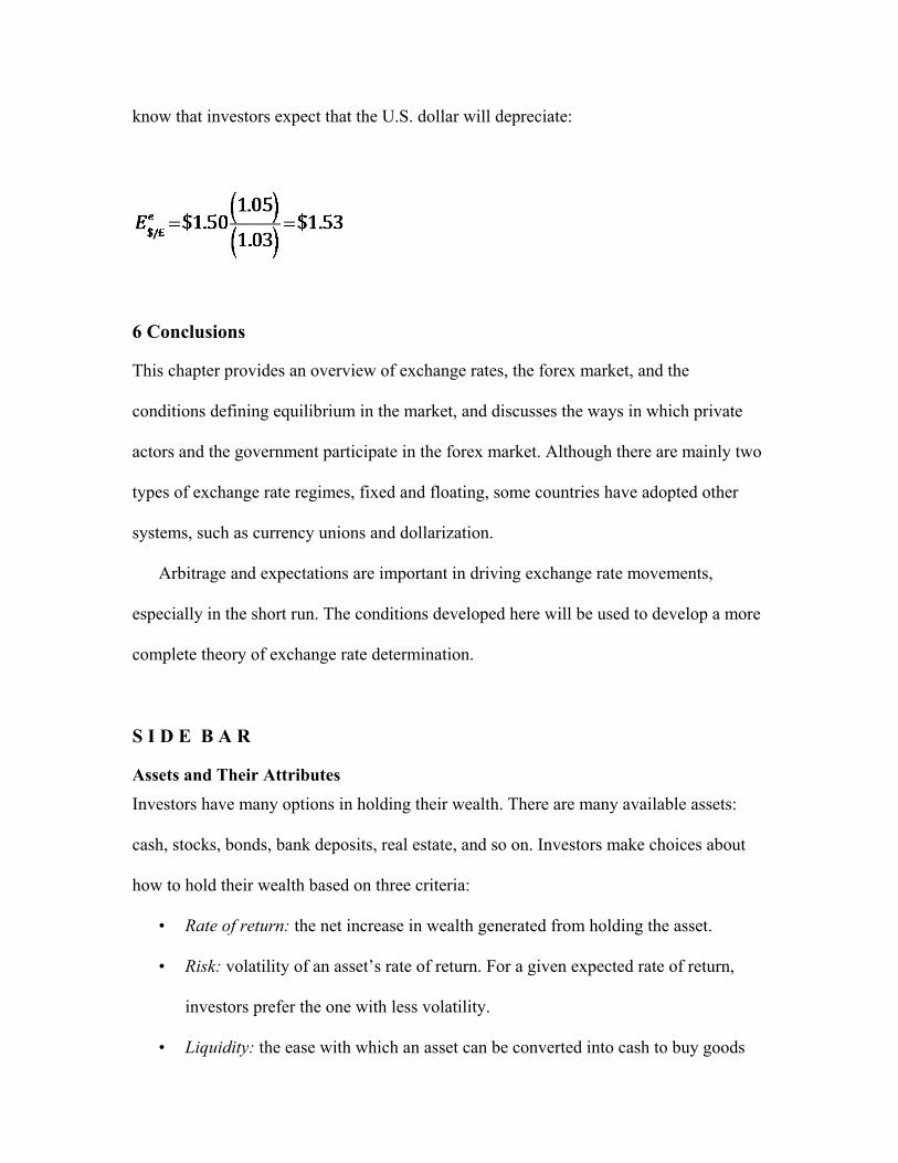
know that investors expect that the U.S. dollar will depreciate:
6 Conclusions
This chapter provides an overview of exchange rates, the forex market, and the
conditions defining equilibrium in the market, and discusses the ways in which private
actors and the government participate in the forex market. Although there are mainly two
types of exchange rate regimes, fixed and floating, some countries have adopted other
systems, such as currency unions and dollarization.
Arbitrage and expectations are important in driving exchange rate movements,
especially in the short run. The conditions developed here will be used to develop a more
complete theory of exchange rate determination.
S I D E B A R
Assets and Their Attributes Investors have many options in holding their wealth. There are many available assets:
cash, stocks, bonds, bank deposits, real estate, and so on. Investors make choices about
how to hold their wealth based on three criteria:
• Rate of return: the net increase in wealth generated from holding the asset.
• Risk: volatility of an asset’s rate of return. For a given expected rate of return,
investors prefer the one with less volatility.
• Liquidity: the ease with which an asset can be converted into cash to buy goods

and services (e.g., the ease with which it can be liquidated or sold). Investors
prefer more liquid assets.
These observations lead to two conclusions. First, investors are willing to trade off more
of one attribute for less of the other(s). That implies that all assets are substitutes for each
other (although they may not be very close substitutes). Second, expectations matter.
Most assets do not have guaranteed rates of return (especially if we look at the real rates
of return). Investors’ forecast of the rate of return is called the expected rate of return.
Teaching Tips
Teaching Tip 1: Uncovered interest parity says the difference between the U.S. interest
rate and the foreign interest rate should equal the expected rate of depreciation of the U.S.
dollar. The Excel workbook for this chapter includes a worksheet that shows comparable
2009 interest rates for a number of countries as well as for the United States. The United
States – foreign difference is also included. Show this table to your students and ask them
to discuss the results. For example, Iceland’s currency is expected to appreciate by
11.24%. Do you believe that result? (Data are from the IMF’s International Financial
Statistics database, accessed December 2010.)
Teaching Tip 2: In this chapter, we assumed frictionless trading in the forex market.
This assumption is relaxed in the last chapter of the textbook. For now, explore the bid-
ask spread with your students. The bid price is the price at which a dealer is willing to
sell a security or currency. The ask price is the willingness-to-buy price. Dealers make a
living on the bid-ask spread. In foreign currency markets, this spread is quoted in pips.
For most currencies, a pip is equal to 0.0001 on the exchange rate. For the yen, however,

one pip is 0.01 of the exchange rate. Exchange rates are conventionally quoted as foreign
currency per U.S. dollar. For example, in the euro–U. S. dollar market, suppose the bid
price is 1.4745 and the ask price is 1.4746. The spread is 1 pip. OANDA’s website offers
a complete list of bid-ask spreads for its trades
(http://fxtrade.oanda.com/why/spreads/recent). You can assign this as an individual or
group project. Either way, have each person or team calculate the round-trip cost of a
trade in which $1,000 (U.S. dollars) are used to buy a foreign currency at the bid price.
The foreign currency is then used to purchase U.S. dollars at the ask price. The difference
between the ending dollar amount and $1,000 is the round-trip cost. (Tell your students to
avoid trades on Saturdays and Sundays because the spreads are larger, reflecting the fact
that forex markets are closed on those days.)
(There are three examples for this chapter in the Excel workbook. OANDA’s website
is loaded with educational material. Begin with http://fxtrade.oanda.com/learn/intro-to-
currency-trading/conventions/ and work through the links on that page. Pay special
attention to http://fxtrade.oanda.com/learn/intro-to-currency-
trading/conventions/currency-pairs and http://fxtrade.oanda.com/learn/intro-to-currency-
trading/conventions/currency-pairs.)
IN-CLASS PROBLEMS
1. Use Table 13-1 in the textbook to answer the following questions:
Exchange Rates on June 30, 2010 Exchange Rates on June 30, 2009
(one year previous)
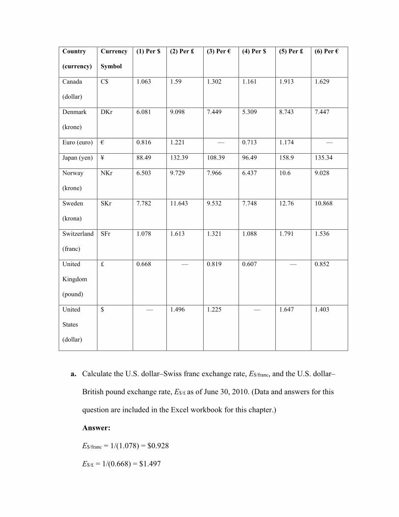
Country
(currency)
Currency
Symbol
(1) Per $ (2) Per £ (3) Per € (4) Per $ (5) Per £ (6) Per €
Canada
(dollar)
C$ 1.063 1.59 1.302 1.161 1.913 1.629
Denmark
(krone)
DKr 6.081 9.098 7.449 5.309 8.743 7.447
Euro (euro) € 0.816 1.221 — 0.713 1.174 —
Japan (yen) ¥ 88.49 132.39 108.39 96.49 158.9 135.34
Norway
(krone)
NKr 6.503 9.729 7.966 6.437 10.6 9.028
Sweden
(krona)
SKr 7.782 11.643 9.532 7.748 12.76 10.868
Switzerland
(franc)
SFr 1.078 1.613 1.321 1.088 1.791 1.536
United
Kingdom
(pound)
£ 0.668 — 0.819 0.607 — 0.852
United
States
(dollar)
$ — 1.496 1.225 — 1.647 1.403
a. Calculate the U.S. dollar–Swiss franc exchange rate, E$/franc, and the U.S. dollar–
British pound exchange rate, E$/£ as of June 30, 2010. (Data and answers for this
question are included in the Excel workbook for this chapter.)
Answer:
E$/franc = 1/(1.078) = $0.928
E$/£ = 1/(0.668) = $1.497

b. What happened to the value of the U.S. dollar relative to the Swiss franc and the
British pound between 2009 and 2010? Calculate the percentage change in the
value of the U.S. dollar relative to each currency using the U.S. dollar–foreign
currency exchange rates you calculated in (a).
Answer: Between those two years, the value of the U.S. dollar depreciated
against the British pound and appreciated against the Swiss franc. The percentage
of appreciation/depreciation in each currency relative to the dollar is given in the
following:
%∆E$/franc = ($0.928 − $0.919)/$0.9191 = 0.0093 = 0.93% appreciation in the
franc vis-à-vis the dollar
%∆EC$/$ = ($1.497 − $1.647)/$1.647 = −0.0913 = 9.13% appreciation in the
pound vis-à-vis the dollar
c. Using the information in the table for the most recent year, calculate the Japanese
yen–Norwegian krone exchange rate.
Answer:
2010: E¥/$ = (88.49¥/(6.503krone/$) = 13.61 krone/ ¥
2. Suppose that the U.S. dollar has appreciated relative to the Chinese yuan and
depreciated relative to the Mexican peso. What has happened to the value of the
dollar based on the effective exchange rate? How is your answer based on the relative
importance of U.S. trade with China and Mexico? Explain.
Answer: When the dollar depreciates against one currency (peso) and appreciates
relative to another (yuan), the effective exchange rate weights the percentage change

in the exchange rates according to how much the U.S. trades with each country.
Because the United States trades more with Mexico than with China (Mexico is the
United States’ second-largest trading partner after Canada), the depreciation will
receive greater weight. Therefore, looking at the effective exchange rate, the U.S.
dollar has depreciated against a basket that includes the peso and the yuan.
3. Use the table below to answer the following questions.
Exchange Rate Quotations
Foreign Currency Units per
U.S. dollar
Country
(currency)
Currency
Symbol
June 30, 2010 June 30, 2005
Brazil (real) BRL 1.7973 2.3555
China (yuan) ¥ (CNY) 6.8086 8.2865
Mexico (peso) MXN 12.8355 10.7630
Data from: http://www.oanda.com.
You and a friend Yi are considering a summer vacation to one of two locales, Mexico
or Brazil. Mexico’s currency unit is the Mexican (new) peso and the real is used in
Brazil. You live in the United States and Yi lives in China. The cost of the hotel is
denominated in local currency units. You and Yi are trying to choose the locale with
the lowest hotel expenses. The price of a hotel room is 200 reals per night in Brazil
and 800 pesos per night in Mexico. Assume these prices remain unchanged between
2005 and 2010.
a. Calculate the U.S. dollar price of a hotel room in Brazil and in Mexico for June
2005. Calculate these prices for 2010. Based on your answers, where would you
spend your vacation in June 2005? In June 2010?
Answer:
The U.S. dollar price of hotel rooms in June 2010:
Brazil: 200 reals per room/1.7973 reals per dollar = $111.28
Mexico: 800 pesos per room/12.8355 pesos per dollar = $117.50
The U.S. dollar price of hotel rooms in June 2005:
Brazil: 200 reals per room/2.3555 reals per dollar = $84.91
Mexico: 800 pesos per room/10.7630 pesos per dollar = $96.54
In both years, the Brazilian hotel has a lower dollar price.
b. For June 2005 and June 2010, calculate the following:
Real–yuan exchange rate, Ereal/yuan
Peso–yuan exchange rate, Epeso/yuan
Answer:
June 2005: Ereal/yuan = Ereal/$/Eyuan/$ = 1.7973/6.8086 = 0.2640 reals per yuan
June 2010: Ereal/yuan = 2.3555/8.2865 = 0.2843 reals per yuan
June 2005: Epeso/yuan = Epeso/$/Eyuan/$ = 12.8355/6.8086 = 1.8852 pesos per yuan
June 2010: Epeso/yuan = 10.7630/8.2865 = 1.2989 pesos per yuan
c. Using your answers from (b) and the information in the table, calculate the
Chinese yuan price of a hotel room in Brazil and in Mexico for June 2005.

Calculate these prices for 2010. Based on your answers, where would Yi prefer to
spend her vacation in June 2005? In June 2010?
Answer:
June 2005 yuan price of hotel room:
Brazil: 200 reals per room/0.2843 reals per yuan = 703.5873 yuan per room
Mexico: 800 pesos per room/1.2989 pesos per yuan = 615.9249 yuan per
room
June 2010 yuan price of hotel room:
Brazil: 200 reals per room/0.2640 reals per yuan = 757.6476 yuan per room
Mexico: 800 pesos per room/1.8852 pesos per yuan = 424.3606 yuan per
room
In both years, Mexico has a lower hotel price. Looks like you and Yi will be
taking separate vacations.
4. Go to the Federal Reserve Bank of St. Louis Economics Database (FRED) and look
up exchange rate data for the following currencies (relative to the U.S. dollar) for the
past four years: Chinese yuan, euro, Brazilian real, and Hong Kong dollar. Are these
exchange rates fixed or floating relative to the U.S. dollar? If the currency is floating
against the U.S. dollar, does the exchange rate change by more than 15% in a given
year?
Answer: The euro and the Brazilian real are floating against the U.S. dollar. The
Hong Kong dollar is fixed against the U.S. dollar. Both the euro and the real have
changed in value relative to the U.S. dollar by more than 10% over the last four years.

While the Chinese yuan is pegged to the dollar, there has been a gradual appreciation
since 2004, totaling 17.47%. (The data for this problem are contained in the Excel
workbook for this chapter, as are graphs of the four exchange rates.)
5. As the volume of transactions in the foreign exchange market grows, how do you
expect this to affect the government’s ability to effectively intervene in the market?
Consider the different tools the government has and their effectiveness in influencing
exchange rates.
Answer: As the volume of transactions increases, the government’s ability to
intervene in the foreign exchange market will be limited. First, the effectiveness of
interventions will be weaker because the government’s interventions will have less of
an effect in a high-volume market. Second, it will be more difficult to enforce and
maintain capital controls on a higher volume of transactions. In this case, there will be
substantial profits associated with the establishment of a black market.
6. Explain how triangular arbitrage works. Why is this important for vehicle currencies
in global markets?
Answer: A triangular trade occurs in the following way. First, the arbitrager buys one
currency, A. Then, she sells A for another currency, B. Finally, she sells B for a third
currency, C. The vast majority of currency pairs are exchanged through a third
currency. This is because some foreign exchange transactions are relatively rare,
which makes it more difficult to exchange currency directly. When a third currency is
used in these types of transactions, it is known as a vehicle currency.

7. In June 2006, a Korean investor is considering investing in bank deposits in Korea
and Japan. The annual interest rate on Korean deposits is 6.25%, versus 3.75% on
deposits in Japan. Suppose that the forward rate in June 2006 is equal to Fwon/¥ = 8.2. In
June 2006, the expected exchange rate is 8.2 won/¥. For the remainder of this question,
please use the linear approximations for uncovered and covered interest rate parity. The
spot exchange rate in June 2006 is Ewon/¥ = 8.
a. Does covered interest parity hold in this example? If so, how do you know?
Calculate the expected return in Japanese deposits (denominated in Korean won)
in this case.
Answer:
CIP: iwon = i¥ + (Fwon/¥ − Ewon/¥)/Ewon/¥
Return on Korean deposits: iwon = 6.25%
Return on Japanese deposit (in won, covered by forward contract): i¥ +
(Fwon/¥ − Ewon/¥)/Ewon/¥ = 3.75% + (8.2 − 8)/8 = 3.75% + 3.13% = 6.88%
Yes, CIP does hold because the return on a Korean deposit is equal to the return
on the Japanese yen deposit (covered by a forward contract).
b. Does uncovered interest parity hold in this example? If so, how do you know? If
not, what is the implied risk premium? Which deposits pay a higher expected
return? Calculate the return on Japanese deposits (denominated in Korean won) in
this case.
Answer:
UIP: iwon + i¥ + (EEwon/¥ − Ewon/¥)/Ewon/¥

iwon = 6.25%
Expected return on Japanese deposit (in won, not covered by forward contract):
i¥ + (EEwon/¥ − Ewon/¥)/Ewon/¥ = 3.75% + (8.25 − 8)/8 = 3.75% + 3.125% =
6.875%
UIP does not hold in this case because the expected returns are not equal.
c. Suppose the exchange rate in June 2007 is equal to 8.528 won per yen. Calculate
the Korean investor’s actual return, assuming that he invests in Japanese deposits
in June 2006. How do these answers compare with those from (b)?
Answer: We know what happened to the won. It appreciated by 6.6% against the
yen.
Actual return on Japanese deposit: i¥ + (E2007won/¥ − E2006won/¥)/E2006won/¥ = 3.75% +
(−6.6%) = –2.85%
If an investor left his deposits in the Japanese bank for the whole year, he would
have earned a loss.
d. Consider two Korean investors: one uses speculation and the other uses hedging.
Based on your previous answers, which one earned a higher return (or smaller
loss) on Japanese assets between June 2006 and 2007? Explain briefly why.
Answer: Although investors expected a depreciation back in June 2006, the won
actually appreciated against the yen between June 2006 and June 2007. Therefore,
speculators who bet on the won depreciation will lose. The investors who hedged
against the depreciation in the won will earn higher returns (or earn relatively
smaller losses).

8. Consider an investor seeking to invest in France. Using the UIP condition (allowing
for risk), explain how each of the following would affect the value of the euro and
U.S. dollar.
a. A decrease in U.S. interest rates
Answer: i$ decreases → return on $ deposits decreases → $ depreciates, €
appreciates, E$/€ increases
b. An increase in France’s interest rates
Answer: i€ increases → return on € deposits increases → $ depreciates, €
appreciates, E$/€ decreases
c. A decrease in the expected future exchange rate, Ee$/€
Answer: Ee$/€ decreases → return on € deposits increases → $ appreciates, €
depreciates, E$/€ decreases
9. Consider the different interest rate parity conditions studied in the chapter. Why
might the exchange rate used in forward contracts differ from the current spot rate?
Why might the forward rate differ from the future spot rate expected by investors?
Explain.
Answer: According to CIP, the difference between the forward rate and the current
spot rate reflects differences in interest rates over time. Because investors can easily
arbitrage away these differences without risk, the CIP holds, but this does not imply
that forward rates and spot rates are equal.
If UIP and CIP hold, then F$/£ = Ee$/£. Therefore, we would expect that the forward
rate and expected future spot rate are equal. If they differ, this would reflect errors in

investors’ forecasts. It is worth noting, however, that UIP involves risky arbitrage—
investors are trading on their forecasts expected exchange rates, without the cover of a
forward contract.

1
2 Trade and Technology: The Ricardian Model
Notes to Instructor
Chapter Summary
The first chapters of this textbook address the question of why countries trade with one another. We will
find that the reasons for trade include differences in technology, resources, cost of offshoring, and
proximity to trading partners.
This chapter addresses the first item above, technology, as an explanation for trade. This reason was first
proposed by David Ricardo, a nineteenth-century economist. Thus, the model is called the Ricardian
model.
The Ricardian model is based on the level of technology in use within nations. As the use of technology
within industries varies, some goods will have a comparative advantage over other goods. Having a
comparative advantage in a good means that a country can produce some goods at a lower opportunity
cost compared with their other goods. The Ricardian model will show that a nation will trade in the good
in which it has the comparative advantage in spite of having an absolute advantage with other nations in
producing all goods.
We will also learn that although comparative advantage will determine patterns of trade, absolute
advantage will determine wages within countries. A nation will pay higher wages for the very reason
that it has an absolute advantage in all goods: If it has better technology, its workers will be more
productive and thus will be paid the value of the resulting higher marginal product.

2
The three key lessons of the Ricardian model are as follows: (1) Comparative advantage determines the
pattern of trade; (2) there are mutual gains from trade; and (3) wages are determined by absolute
advantage.
As a sidenote, the snowboard example in the beginning of the chapter serves as an introduction to all the
trade chapters (Chapters 2–7), allowing the instructor to skip Chapter 1 if desired. Keep in mind, though,
that Chapter 1 provides a good overview of who trades with whom and by how much in the real world.
It is also a good overview of the international trade topics that this book discusses. Chapter 1 provides
an excellent background and springboard for students that may help to guide them toward an
understanding of what international trade is really all about today. Too often, we assume it is only about
goods traded across borders, but much more is traded in the factors of production, like capital. And
migration has become a controversial issue as well, and this chapter makes clear why migration is
fundamentally an international trade issue. This material may also help students to connect what they
read in the news with the international trade topics covered in this text. Chapter 1 also offers a good
historical perspective, suggesting that globalization and interconnectedness are not new to the
international stage. In essence, the material in Chapter 1 will connect students to today’s international
trade issues and challenges, while providing an overview of what international trade entails and what
will be covered in this text. However, if you are short on time, this is probably the one chapter that could
be skipped.
Comments
Although most students may be familiar with the concept of comparative advantage from principles of
microeconomics, it is a good idea to reintroduce this concept because many students find it challenging.
This chapter also provides a more in-depth analysis of the Ricardian model by covering the

3
determination of relative prices as well as the relationship between wages and absolute advantage. The
latter is particularly interesting as it is not covered in most trade textbooks. A corresponding application
provides convincing evidence regarding a country’s level of technology and wages.
Lecture Notes
Introduction
Most manufactured products are traded between countries, including the snowboard. In 2014, the United
States imported 350.6 thousand snowboards worth $28.2 million from 18 different countries. The top 12
countries selling snowboards to the United States are shown in Table 2-1, with China at the top of the
list, followed by Austria, the United Arab Emirates, Taiwan, Canada, Switzerland, Germany, Slovenia,
the Netherlands, France, Tunisia, and Slovak Republic. But, why does the United States purchase
snowboards from these countries at all when it already has the resources and technology to produce the
snowboards?

4
To answer this question and understand why countries trade goods with each other, we will examine the
reasons for trade. These trade determinants include proximity (geographic distance between countries),
resources (land, labor, and capital), offshoring, and differences in level of technology.
This chapter focuses mainly on the latter reason, technological differences across countries, and will use
the “Ricardian model” named for nineteenth-century economist David Ricardo to explain trade between
countries with differing levels of technology. The level of technology used by a country will determine
the pattern of trade as well as the wages paid to labor.
1 Reasons for Trade
Proximity The proximity of Canada to the United States means lower transportation costs relative to

5
trade between the United States and countries in Asia or Europe. This close distance between the two
neighboring countries may explain why Canada is not only one of the top exporters of snowboards to the
United States, but also one of its largest trading partner overall. Proximity may additionally be the
reason why Europeans countries mainly trade with each other, whereas Japan or China is the largest
trading partner for many Asian countries. Countries located in close proximity of one another often join
free-trade areas to promote trade by eliminating barriers to trade such as tariffs and quotas.
Resources Resources are another reason that helps to explain why nations trade with one another.
Consider Austria that sells some 30 times more in value to the United States than does Canada, in spite
of Canada being significantly closer. And Mexico (included in the “All other countries” category) sells
only some $6,000. How do we explain why Austria and Canada sell so much more than Mexico?
The reason may lie in the fact that, in contrast to Mexico, both Austria and Canada have cold snowy
mountains ideal for snowboarding. Austria and Canada’s geographic resource provides another reason
for trade. Other resources are land, which also provides minerals; labor resources of various education
and skills; and capital, such as machinery and infrastructure. Land, labor, and capital are often referred
to as factors of production because these resources are used to produce goods and services. Favorable
geographic conditions also help to explain the appearance of some of the other top 12 exporters of
snowboards to the United States, namely, Switzerland, Germany, Slovenia, and France.
And it is important to note that a country can create a comparative advantage. Consider Germany’s
invention of ice wine, which is now also produced in the Niagara Falls region of Canada (see Side Bar:

6
Can Comparative Advantage Be Created?). The United Arab Emirates is another such example, with a
Ski Dubai indoor ski center having opened there. The country has since initiated an industry that
produces high-quality snowboards.
The lower-priced snowboards from Canada ($18) and Mexico ($14) may be indicative of companies
selling unfinished boards that require further processing. The process of trading unfinished goods and
spreading production across several countries is called offshoring. This type of trade is covered in
Chapter 7.
Absolute Advantage Although Germany also has a natural resource, the Alps on its southern border,
the reason it is the seventh largest exporter of snowboards to the United States may be better explained
by its advanced technology. As a world leader in the production of many manufactured goods, Germany
has an absolute advantage in producing snowboards because it has the best technology to produce the
good. Germany is known for producing many products, including machine tools, motor vehicles, and
steel products that require high levels of technology.
However, this raises the question as to why the United States imports about 4 times more snowboards
from China, a country with less-advanced technology relative to Germany. Indeed, it is also puzzling
why the United States, with technology equal to that of Germany, would import snowboards from either
country, rather than producing snowboards on its own.
S I D E B A R
Can Comparative Advantage Be Created? The Case of “Icewine”
By linking the production of “icewine,” first developed in Germany in 1794, to the cold climate of its

7
Niagara Falls region, Canada is able to create a new comparative advantage in producing this sweet
dessert wine.
Comparative Advantage To determine trade patterns, we need to examine the relative rather than
absolute differences in technology between countries. To gain a better understanding of the topic, we
turn to the concept of comparative advantage, introduced by David Ricardo using a simple example
consisting of two countries (Portugal and England) trading two goods (wine and cloth). Ricardo allowed
Portugal to have the best technology or absolute advantage in the production of both goods. In contrast,
although England is capable of producing both goods, it is relatively more difficult for England to
produce wine. Given Ricardo’s assumption that England is better at producing cloth than wine, England
has a comparative advantage in the production of cloth and should export cloth to Portugal. In exchange
for the cloth from England, Portugal should export wine because it has a comparative advantage in the
production of that good.
The concept of comparative advantage may explain why the United States imports more snowboards
from China than Germany, even though China has less-advanced technology in the production of
snowboards relative to Germany or the United States. The remainder of the chapter provides more detail
about this fundamental theory in international trade.
S I D E B A R
David Ricardo and Mercantilism
David Ricardo introduced the concept of comparative advantage as the basis for trade in response to the
mercantilist school of thought that a country should actively export while preventing imports with high

8
tariffs on foreign goods. Assuming that countries have balanced trade, Ricardo showed that these
countries could benefit by engaging in free trade. Ricardo’s ideology of trade without barriers is the
foundation of many international institutions, such as the United Nations, World Bank, and World Trade
Organization (WTO).
2 Ricardian Model This section provides a detailed example of the Ricardian model with the home
country trading wheat and cloth. We will find that absolute advantage is not a good reason for trade and
that a better understanding of trade comes from a good understanding of comparative advantage within a
nation. The comparative advantage model will show that the home country (Home) should export wheat
and import cloth in spite of being able to produce both wheat and cloth cheaper than its trading partners.
The Home Country To gain a better understanding of the main concepts of the Ricardian model, we
simplify the example by assuming that labor is the only factor of production for both goods. We use the
information that one worker at Home can produce 4 bushels of wheat or 2 yards of cloth per hour. The
marginal product of labor (MPL) of each good per hour at Home is then given by MPLW = 4 · MPLC =
2.
Home Production Possibilities Frontier Suppose that there are = 25 workers in the home country.
We will begin by plotting Home’s production possibilities frontier (PPF). To graph the PPF, we
calculate the maximum bushels of wheat Home could produce in an hour if all workers were employed
in producing wheat. They could produce QW = MPLW · = 4 · 25 = 100 bushels of wheat per hour. If
instead all workers were employed in cloth, then they could produce QC = MPLC · = 2 · 25 = 50 yards

9
of cloth per hour. Connecting the two production points gives us the straight-line PPF unique to the
Ricardian model, as shown in Figure 2-1. The PPF is a straight line because the marginal products of
labors are constant, a result of the earlier assumption that production does not include land and capital.
This means that there are no diminishing returns in the Ricardian model.
The slope of the PPF, equal to the ratio of the marginal products in the two goods, gives the opportunity
cost of one good (on horizontal axis) in terms of the other (on vertical axis).
Slope of 𝑃𝑃𝑃𝑃𝑃𝑃 = 50100
= 𝑀𝑀𝑀𝑀𝑀𝑀𝑐𝑐 · 𝑀𝑀𝑀𝑀𝑀𝑀𝑀𝑀𝑤𝑤 · 𝑀𝑀
=𝑀𝑀𝑀𝑀𝑀𝑀𝑐𝑐𝑀𝑀𝑀𝑀𝑀𝑀𝑤𝑤
= −12
The slope of the PPF gives the opportunity cost of 1 bushel of wheat in terms of cloth. The slope of − 12
means that Home gives up 12
yard of cloth to increase the output of wheat by 1 bushel. To see this,
notice that home country must give up one quarter of a worker’s time to produce cloth to obtain 1
bushel of wheat. By shifting the 15 minutes from cloth to wheat, Home reduces cloth output by 12
yard.

10
Thus, 12
yard of cloth is the opportunity cost of obtaining one more bushel of wheat and this is exactly
the slope of the PPF.
You might point out to students that to calculate the opportunity cost of a good (in the denominator) in
terms of the other good (in the numerator), the units will always be in the units of whatever is in the
numerator. This always causes confusion for students.
Home Indifference Curve To determine the level of wheat and cloth production, we examine Home’s
demand for the two goods, as represented by the country indifference curves. Similar to indifference
curves representing individual preferences, an indifference curve for a country reflects higher levels of
utility the further away it is from the origin. In addition, Home is indifferent between any two
combinations of wheat and cloth on the same indifference curve. For example, in Figure 2-2, the
consumer is indifferent between points A and B. But, at point C, a higher indifference curve indicates
that a higher level of utility is possible. In Figure 2-2, we are examining the entire nation and
considering the preferences of the entire country. Notice that utility at U0 represents a lower level of
utility for all consumers in the country.

11
Home Equilibrium Without international trade, Home will produce at the point where the indifference
curve is just tangent to the PPF, which acts like the country’s budget constraint. Figure 2-2 shows that
Home achieves the most satisfaction at the “no-trade” or the “pre-trade” equilibrium denoted by point A,
at which U1 represents the highest indifference curve Home can obtain by having its own firms produce
and sell the two goods under perfect competition.
The highest level of utility that can be achieved in Figure 2-2 is at point A, where Home produces 25
yards of cloth and 50 bushels of wheat. This is the Autarky or no international trade position. This point
assumes a competitive market, with many firms as price takers. This price for wheat and cloth is
therefore given, and point A represents the highest level of well-being possible and is an example of
Adam Smith’s invisible hand at work.
Opportunity Cost and Prices Under perfect competition, at the no-trade equilibrium, the opportunity

12
cost and relative price of wheat (on horizontal axis) are equal. This result follows from assuming that
labor is perfectly mobile between the two industries and that firms will hire labor up to the point where
wage in an industry equals the price of the good times the marginal product of labor in the sector
producing the good.
We will now show that this equality between the opportunity costs and the relative price of wheat holds
at point A.
Wages With labor freely able to move between the industries, wages across the industries must be equal,
which gives the equality of the price ratio with the ratio of the marginal products in the two goods.
Setting wage equal in the two sectors
· wage ·W W C CP MPL P MPL= =
and rearranging gives
The right side is the slope of the PPF, which also is the opportunity cost of wheat in terms of cloth,
whereas the left side is the relative price of wheat. Substituting the marginal product of labor in wheat
and cloth, we find that the relative price of wheat in the home country without international trade is
equal to 12
(PW/PC = MPLW/MPLC = 12
).

13
The price ratio (PW/PC ) denotes the relative price of the good in the numerator and is measured in terms
of how much of the good in the denominator must be given up. Thus, PW/PC is the relative price of
wheat, which is on the horizontal axis. Note that the relative price of wheat represents the slope of the
PPF.
The Foreign Country We have seen the equilibrium in both countries in the absence of trade. Now let’s
see what happens when trade begins. The lesson we will learn is that each country will export that good
in which it has a comparative advantage over its trading partner, even though it may have an absolute
advantage in both goods. This means that patterns of trade are determined, in the Ricardian model, by
the opportunity costs of production.
In our model, the foreign country is assumed to have an inferior technology, or an absolute disadvantage
in producing both wheat and cloth, as compared with Home. In particular, one worker can produce 1
bushel of wheat or 1 yard of cloth. Thus, the marginal product of labor in wheat and cloth in Foreign
are 𝑀𝑀𝑃𝑃𝑀𝑀 𝑊𝑊∗ = 1 and 𝑀𝑀𝑃𝑃𝑀𝑀 𝐶𝐶∗ = 1, respectively.
With = 100, Foreign is able to produce a maximum of 𝑀𝑀𝑃𝑃𝑀𝑀 𝑊𝑊∗ · 𝑀𝑀 = 100 bushels of wheat per hour
if all workers were producing wheat. If instead all workers were employed in cloth production, Foreign
would be able to produce a maximum of 𝑀𝑀𝑃𝑃𝑀𝑀 𝐶𝐶∗ · 𝑀𝑀 = 100 yards of cloth per hour.

14
Foreign Production Possibilities Frontier The Foreign PPF, given in Figure 2-3, is the straight line
between the two Foreign production points. The slope of the Foreign PPF, measured by the ratio of the
marginal products in the two goods, is −1. We will now turn to the concept of comparative advantage to
understand why the United States, with its superior technology in the production of both wheat and
cloth, would import most of its clothing from countries in Asia and Latin America.
Comparative Advantage The opportunity cost of 1 bushel of wheat in terms of yards of cloth in the
foreign country is equal to 1. But, the opportunity cost of 1 bushel of wheat in terms of yards of cloth in
the home country (𝑀𝑀𝑀𝑀𝑀𝑀𝑊𝑊𝑀𝑀𝑀𝑀𝑀𝑀𝐶𝐶
= 12) is lower than that in the foreign country (𝑀𝑀𝑀𝑀𝑀𝑀𝑊𝑊
∗
𝑀𝑀𝑀𝑀𝑀𝑀𝐶𝐶∗ = 1) . This means that
Home gives up less cloth to produce 1 bushel of wheat than Foreign. Because Home has a lower
opportunity cost of producing wheat than Foreign, Home has a comparative advantage in producing
wheat, whereas Foreign has a comparative advantage in producing cloth (𝑀𝑀𝑀𝑀𝑀𝑀𝐶𝐶𝑀𝑀𝑀𝑀𝑀𝑀𝑊𝑊
= 2 > 𝑀𝑀𝑀𝑀𝑀𝑀𝐶𝐶∗
𝑀𝑀𝑀𝑀𝑀𝑀𝑊𝑊∗ = 1),
because its opportunity cost of producing cloth is lower than Home’s opportunity cost. A country has a

15
comparative advantage in a good when it is able to produce the good at a lower opportunity cost than its
trading partner. Importantly, we get this result despite the assumption that Home has an absolute
advantage in the production of both goods.
Applying the same methodology for Home, we include Foreign’s preferences for wheat and cloth with
indifference curves to obtain the no-trade equilibrium. Figure 2-4 shows that under competitive markets,
Foreign will produce at point A*, at which it achieves the highest level of utility. The slope of the foreign
PPF gives us the relative price as well as the opportunity cost of wheat without trade
( ). The comparative advantage that the home country has in the production of
wheat is also reflected by the lower relative price of wheat at Home (PW/PC = 12
), compared with
Foreign.

16
APPLICATION
Comparative Advantage in Apparel, Textiles, and Wheat
Table 2-2 shows that a worker in the United States generates 2.6 times more apparel sales and 12 times
more textiles sales per year than a worker in China. With its absolute advantage in the production of
both industries, why does the United States import apparel and textiles from China and other Asian
countries? The answer has to do with the fact that a typical wheat farmer in the United States is 33 times
more productive than a farmer in China. With its absolute and comparative advantage in the production
of grain, the United States exports grain to China in exchange for apparel and textiles, as predicted by
the Ricardian model.

17
3 Determining the Pattern of International Trade
International Trade Equilibrium We now examine why the two countries participate in international
trade. Because the relative price of wheat in the home country (PW/PC = 12
) is lower than the relative
price of wheat in the foreign country ( ), producers of wheat at Home would want to export
wheat to Foreign. Conversely, producers of cloth in the foreign country would want to export cloth since
the relative price of cloth is higher in the home country (PC/PW = 2) than the foreign country
( ). Therefore, differences in no-trade prices provide an incentive for the two countries to
trade.
As predicted by the Ricardian model, both countries export the good in which they have a comparative
advantage. This is the fundamental law that determines trade patterns in the Ricardian model.
International trade equilibrium between the two countries occurs only when the relative price of wheat
(or cloth) is the same across the countries. This occurs because as Home exports wheat, the supply of
wheat in the home country falls, bidding up the price, while the supply of wheat in the foreign country
increases, bidding down the price, leading to a higher relative price at Home and a lower relative price at
Foreign. Similarly, the foreign country’s export of cloth drives up the relative price of cloth in Foreign
as supply decreases and leads to a fall in the relative price at Home. In the next section, we will
determine the relative price of wheat at the trade equilibrium and examine how the change in the relative
price of wheat, due to trade, affects production and consumption in each of the countries.

18
Change in Production and Consumption We must address two questions to fully understand the
international trade position:
1. What will be the relative price of wheat (cloth) in the trade equilibrium?
2. How does trade impact production and consumption in both Home and Foreign?
We will address the second question first and assume a relative price has been established. To determine
how trade impacts each country’s production and consumption patterns, we begin by supposing that the
international relative price of wheat is equal to 23
, which is in-between Home’s ( 12
) and Foreign’s (1)
no-trade relative price. Given the higher international relative price of wheat ( 23
> 12
), producers in the
home country would want to export wheat abroad and all workers would want to work in the wheat
industry.
To see that workers at Home would receive a higher wage working in the wheat industry than the cloth
industry, we compute the ratio of wages in the two industries using the international relative price of
wheat (PW/PC = 23
), and the marginal product of labor for cloth = MPLC (2) and wheat = MPLW (4):
Wage𝑤𝑤Wage𝑐𝑐
= 𝑃𝑃𝑤𝑤 · 𝑀𝑀𝑃𝑃𝑀𝑀𝑤𝑤𝑃𝑃𝐶𝐶 · 𝑀𝑀𝑃𝑃𝑀𝑀𝑐𝑐
= (23
)(42
) =86
> 1, which implies 𝑃𝑃𝑤𝑤 · 𝑀𝑀𝑃𝑃𝑀𝑀𝑤𝑤 > 𝑃𝑃𝐶𝐶 · 𝑀𝑀𝑃𝑃𝑀𝑀𝑐𝑐
Because of the higher wages in the wheat industry, no cloth is produced and the home country fully
specializes in the production of wheat, as occurs at point B in Figure 2-5. This fully specialized position

19
is due to the straight line for the PPF.
International Trade Starting from Home’s production point (point B in Figure 2-5), we know that with
the international relative price of wheat at 23
, Home can export 1 bushel of wheat in exchange for 23
yard of cloth from Foreign. Tracing out Home’s international trade gives the international trade line
shown as BC in Figure 2-5. The international trade line implies a “new” budget constraint for the home
country that has a steeper slope (− 23
) than Home’s PPF. This line, BC, is the world price line and is
equal to the negative of the world relative price. This world price line represents the consumption
possibilities that the nation is able to reach by specializing in only one good and then engaging in trade.
This, in essence, allows the country to experience a higher budget constraint under international trade.

20
Home’s budget constraint is above its pre-trade PPF budget constraint and is thus able to choose a
consumption point (point C) that is on a higher indifference curve (U2). Therefore, Home gains from
trade by obtaining a higher utility with international trade than under no-trade.
Pattern of Trade and Gains from Trade With the international relative price of wheat at 23
, Home
produces 100 bushels of wheat (point B) but consumes only 40 bushels (point C). The extra 60 bushels
are exported to the foreign country in exchange for 40 yards of cloth imported from Foreign. The value
of the wheat in terms of cloth is determined by multiplying the international relative price of wheat by
the amount of wheat export, ( 23
) · 60 = 40 yards of cloth. Because the value of exported wheat is equal
to the value of imported cloth, trade in the home country is balanced.
The results for the foreign country produce trade patterns that are opposite those of the home country
because the international relative price of wheat is less than the foreign no-trade relative price of wheat.
These results are shown below in Figure 2-6. Workers in the foreign country will flock to the cloth
industry as producers in this industry take advantage of the higher international relative price of cloth
(reciprocal of the international relative price of wheat) to export cloth. Foreign becomes fully
specialized in the production of cloth, denoted by point B* in Figure 2-6. Tracing out Foreign’s
international trade at the exchange of 23
yards of cloth for 1 bushel of wheat gives the international
trade line, B*C*, which equals the negative of the slope of the international relative price of wheat ( 23
)
and is flatter than Foreign’s PPF. The foreign country also gains from trade by acquiring a higher utility
given by the tangency of indifference curve 𝑈𝑈𝐶𝐶∗ with the international relative price of wheat at point C*.

21
Similar to the home country, trade in the foreign country is also balanced. By specializing in the
production of cloth, Foreign produces 100 yards, 60 of which it keeps for consumption and the other 40
it exports to Home in exchange for 60 bushels of wheat. Note that the amount of cloth Foreign exports is
exactly equal to the 40 yards that Home imports. Likewise, Foreign imports 60 bushels of wheat, which
is the same amount that Home exports.
With international trade, the home country exports wheat, in which it has a comparative advantage, and
the foreign country exports cloth because it has a comparative advantage in cloth. Both countries enjoy
mutual gains from trade by consuming at a higher level of utility relative to their no-trade levels. These

22
two findings are consistent with the Ricardian model, where the pattern of trade is determined by
comparative advantage and both countries gain from trade.
A very important third lesson can be inferred from the Ricardian model. We have just learned that prices
for the goods converge to a single equilibrium price. Is this also true for wages? Do wages converge to a
single value across trading partners? The Ricardian model does not predict this. Even though trading
patterns are determined by comparative advantage, wage determination within the countries is
determined by absolute advantage within each nation. We will address this important corollary next.
Solving for Wages Across Countries In this section, we examine the relationship between absolute
advantage and how wages are determined across countries. At Home, workers are paid in terms of wheat
because the home country produces and exports this good. The workers could either consume their
“real” wage, measured in terms of wheat, or exchange for cloth with Foreign at the international relative
price of PW/PC = 23
. Wages at Home are summarized by the following:
MPLW = 4 bushels of wheat
Home wages = or
(PW/PC) · MPLW = 83
yards of cloth
In the foreign country, workers are paid in terms of cloth as Foreign produces and exports cloth. The real
wage of workers in Foreign is 𝑀𝑀𝑃𝑃𝑀𝑀𝐶𝐶∗ = 1 yards of cloth, which they can either consume or trade for
wheat in the international market. Cloth workers sell their product on the world market for 32
bushels.

23
This means that their real wage in terms of wheat is 32
bushels. Foreign wages are summarized by the
following:
(P*C/P*W) · 𝑀𝑀𝑃𝑃𝑀𝑀𝐶𝐶∗ = 32
bushels of wheat
Foreign wages = or
𝑀𝑀𝑃𝑃𝑀𝑀𝐶𝐶∗ = 1 yards of cloth
Wages across the countries depend on the marginal products of labor and the international trade relative
price of the goods.
Absolute Advantage Note that the because Home has an absolute advantage in both goods, Foreign
workers earn less than Home workers, as made evident by how much less they can purchase of either
good—1 yard of cloth or 32
bushels of wheat compared to Home’s ability to purchase 83
yards of cloth
or 4 bushels of wheat. Home workers can afford to purchase more of wheat and cloth than Foreign
workers because the home country has an absolute advantage in the production of both goods. This is
implied by the Ricardian model. Since trade is determined by comparative advantage, if a country has
poor technology, the only way that it can compete and sell at a price that Home is willing to pay is if
Foreign’s wages are lower.
This does not imply that for developing countries, trade will only occur if wages are low. In fact, as
trade progresses and the country begins to develop, so, too, will its technology. As it becomes more
technologically advanced and thus more productive, its wages will begin to increase as well. The

24
Ricardian model predicts this very scenario.
Data support this theory as both China and India have experienced it. After 36 years of international
trade in China, the nation’s per capita income by 2014 had increased nearly 8 times from $1,600 to
$12,400, implying that the real income of Chinese consumers doubled every 12 years. Similarly, in
India, its per capita income increased 4 times in 36 years of international trade from $1,300 to $5,600,
implying that real income doubled every 18 years.
APPLICATION
Labor Productivity and Wages
Using value-added per hour as the measure for labor productivity, we see from Figure 2-7 that there is a
relationship between labor productivity and wages. Of the seven countries presented, the United States
has the highest level of productivity and enjoys the highest wage, whereas Taiwan has the lowest level
of productivity and thus receives the lowest wage. Figure 2-8 shows the labor productivity and wages
over time for each of the seven countries. The graphs indicate a close connection between labor
productivity and wages, with both rising over time.

25

26
4 Solving for International Prices
Instead of assuming that the international relative price of wheat is between the two countries’ no-trade
relative prices as we did in the previous section, we now solve for it using supply and demand curves,
in which the world supply curve is derived from the Home export supply curve, whereas the world
demand curve is derived from the Foreign import demand curve. The intersection of the export supply
curve and the import demand curve determines the international prices.
Home Export Supply Curve We use panel (a) of Figure 2-9, which is a replica of Figure 2-5, to
construct the Home export supply curve, in which the vertical axis measures the relative price of wheat
and the horizontal axis measures the exports of wheat. The export supply curve of wheat is equal to zero
when the international relative price of wheat is below the home country’s no-trade price ratio ( 12
).
When the international relative price of wheat is equal to the home country’s no-trade price ratio, the
export supply curve is flat, starting from zero to the home country’s no-trade consumption point [points
A' and B' in panel (b) of Figure 2-9 corresponding with points A and B in panel (a)]. At the international
relative price of wheat ( 23
), Home could be entirely self-sufficient by producing and consuming at point
A or it could completely specialize in the production of wheat by producing 100 bushels at point B.
Because Home consumes only 40 bushels of wheat, the rest are exported to Foreign in exchange for 40
yards of cloth. In addition, with wages equal across the two industries, workers can freely move from
one industry to another so that Home would produce on any point on the PPF between A and B. If the
international relative price of wheat is 23
, we know from the earlier analysis that Home exports 60
bushels of wheat, corresponding with point C' in panel (b). The export supply curve rises as the relative

27
prices of wheat increase.
Foreign Import Demand Curve Using the same reasoning, the import demand curve for wheat is equal
to zero when the international relative price of wheat is above the foreign no-trade relative price of
wheat. If the international relative price of wheat is equal to 1, Foreign could either consume all of the
wheat and cloth it produces on its own [points A* and A*′ in panels (a) and (b) of Figure 2-10,
respectively] or specialize in the production of cloth by producing 100 yards and exporting 50 yards to
the home country [points B* and B*′ in panel (a) and points A*′ and B*′ in panel (b)]. Because wages are
equal across the two industries, Foreign could produce anywhere on its PPF between points A* and B*,
which gives the flat segment of the import demand curve when the international relative price of wheat
equals the foreign country’s no-trade relative price. As the relative price of wheat decreases, for
example, from 1 to 23
, the foreign country will specialize in cloth and import more wheat, leading to the

28
downward-sloping import demand curve for wheat. The flat portion of the import demand is unique to
the Ricardian model because of the straight-line production possibilities frontier.
International Trade Equilibrium Combining the Home export supply curve and the Foreign import
demand curve gives the world market for wheat, as shown in Figure 2-11. The intersection of the world
supply and demand curves, denoted by point C′, gives the international trade equilibrium, in which the
Home export of wheat is equal to Foreign import of wheat at the equilibrium relative price of wheat.

29
The Terms of Trade This is defined as the price of a country’s exports divided by the price of its
imports. The home country’s terms of trade, defined by PW/PC, improve as the price of wheat increases
or as the price of cloth falls. This means that the home country is able to purchase more cloth while
exporting the same amount of wheat. For the foreign country, its terms of trade (PC/PW) rise following a
higher price of cloth (its export) or a lower price of wheat (its imports). The terms of trade can make a
country better off (earning more for exports or less for imports) or worse off (earning less for exports or
paying more for imports).
APPLICATION
The Terms of Trade for Primary Commodities
In 1950, economists Raúl Prebisch and Hans Singer hypothesized that over time, the price of primary
commodities such as agricultural products and minerals would decline relative to the price of
manufactured goods. The decline of primary commodities would lead to a worsening of the terms of
trade for developing countries, the source of most of these products. The three graphs in Figure 2-12
show that the relative price of primary commodities has increased, decreased, and remained roughly the

30
same over time, depending on the product traded.
5 Conclusion
The Ricardian model consists of the simple concept that the pattern of trade is determined by
comparative advantage. By exporting the good in which a country has the lowest opportunity cost
relative to producing another good, the country could benefit from participating in international trade by
consuming at a higher level of utility than it would under no trade. In addition, the Ricardian model also
shows that wages across countries are determined by absolute advantage, in which the country

31
possessing the more advanced technology will enjoy higher real wages. Another result of the Ricardian
model is that a small country will gain from trading with a large country, but the larger country will
neither gain nor lose from the trade. The reason is because the international equilibrium price ratio will
equal the large country’s relative no-trade prices.
TEACHING TIPS
Tip 1: Comparative Advantage
Comparative advantage is perhaps the most important concept in international trade. Therefore, it
warrants substantial treatment in this course. Ask students to break into groups or work on their own to
come up with additional example of comparative advantage that need not relate to international trade.
Discussing examples, such as lawyers paying landscapers to mow their lawns, may help students better
grasp the concept.
Tip 2: An Introduction to Trade Data
To familiarize students with international trade data and sources, have students explore the part of the
United States International Trade Commission website that accesses trade data
(http://dataweb.usitc.gov/prepared_reports.asp). Direct students to explore U.S. trade balances sectors,
noting any trends they might find. Ask them to consider what role comparative advantage might play in
the trends they observe.
Tip 3: Individual Products, Trade Flows, and Comparative Advantage
Yet another way to engage students in empirical international trade is to ask them to look up specific

32
goods and the United States’ major trading partners. Have your class go to the website of the
International Trade Administration at the U.S. Department of Commerce
(http://www.trade.gov/mas/ian/otii/index.asp). Students can then follow the TradeStatsExpress link
(scroll down and click on the icon), next click on National Trade Data, and finally click on Global
Patterns of U. S. Merchandise Trade.
Here, students can pick their own goods to investigate U.S. imports, exports, and trade balance. Ask
them to look up a good they expect the United States to have a comparative advantage or disadvantage
in and to test their beliefs with current data.
Some examples of goods and their harmonized system codes follow. After students click the “Change”
button under “Product,” tell them to be sure to click the “HS Radio” button before they look for “HS
Codes.” To enter the six-digit codes below, they will need to click the “Product Code” tab in the “Select
Products for Report” dialog box.
Harmonized System
Codes (HS Codes)
Product Description
880240 Airplanes and other aircraft, of an unladen weight
exceeding 15,000 kilograms
480300 Toilet or facial tissue stock, towel or napkin stock
and similar paper of a kind used for household or
sanitary purposes, cellulose wadding and webs
660110 Garden or similar umbrellas

33
Harmonized System
Codes (HS Codes)
Product Description
920300 Keyboard pipe organs; harmoniums and similar
keyboard instruments with free metal reeds
180100 Cocoa beans (whole or broken)
IN-CLASS PROBLEMS
1. What determines the pattern of international trade between two countries in the Ricardian model?
Answer: The pattern of trade is determined by comparative advantage. The country with a
comparative advantage in the production of a product will export the good.
2. Using the Ricardian model, explain why American workers receive higher wages in the production
of automobiles than Chinese workers.
Answer: American automobile workers receive higher wages than Chinese automobile workers
because the United States has an absolute advantage in the production of many goods, including
automobiles.
3. Why is the production possibilities frontier a straight line in the Ricardian model?
Answer: The production possibilities frontier is a straight line in the Ricardian model because of the
assumption that the marginal products of labor are constant. The Ricardian model ignores the role of

34
land and capital, so there are no diminishing returns.
4. Refer to the following table and assume that the total labor supply in Taiwan is 4 and the total labor
supply in Vietnam is 8.
Taiwan Vietnam Absolute
Advantage
Number of
telephones produced
per hour
10 5 ?
Number of radios
produced per hour
50 10 ?
Comparative
advantage
? ?
a. What is the opportunity cost of 1 unit of telephones in terms of radios in Taiwan? In Vietnam?
Answer: See the following table.
Opportunity Cost of
1 Telephone (in Terms
of Units of Radio
Given Up)
1 Radio (in Terms of Units
Telephone Given Up)
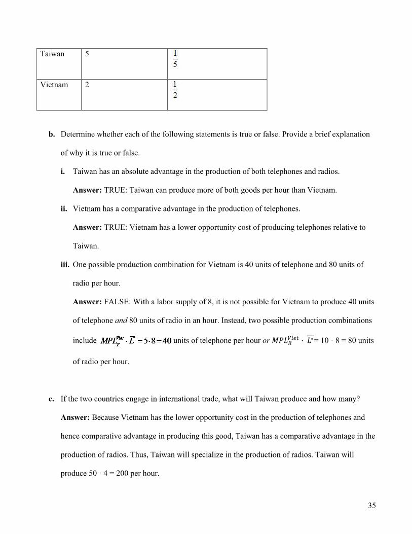
35
Taiwan 5
Vietnam 2
b. Determine whether each of the following statements is true or false. Provide a brief explanation
of why it is true or false.
i. Taiwan has an absolute advantage in the production of both telephones and radios.
Answer: TRUE: Taiwan can produce more of both goods per hour than Vietnam.
ii. Vietnam has a comparative advantage in the production of telephones.
Answer: TRUE: Vietnam has a lower opportunity cost of producing telephones relative to
Taiwan.
iii. One possible production combination for Vietnam is 40 units of telephone and 80 units of
radio per hour.
Answer: FALSE: With a labor supply of 8, it is not possible for Vietnam to produce 40 units
of telephone and 80 units of radio in an hour. Instead, two possible production combinations
include units of telephone per hour or 𝑀𝑀𝑃𝑃𝑀𝑀𝑅𝑅𝑉𝑉𝑉𝑉𝑉𝑉𝑉𝑉 · 𝑀𝑀∗= 10 · 8 = 80 units
of radio per hour.
c. If the two countries engage in international trade, what will Taiwan produce and how many?
Answer: Because Vietnam has the lower opportunity cost in the production of telephones and
hence comparative advantage in producing this good, Taiwan has a comparative advantage in the
production of radios. Thus, Taiwan will specialize in the production of radios. Taiwan will
produce 50 · 4 = 200 per hour.

36
d. What is the real wage in Taiwan in terms of radio? What is the real wage in Vietnam in terms of
telephone?
Answer: The real wage in Taiwan in terms of radio is units of radio. The real wage
in Vietnam in terms of telephone is 𝑀𝑀𝑃𝑃𝑀𝑀𝑇𝑇𝑉𝑉𝑉𝑉𝑉𝑉𝑉𝑉 = 5 units of telephone.
e. Will Taiwan and Vietnam trade if the international relative price of telephone is 3? Briefly
explain why or why not.
Answer: Because the no-trade prices are in Taiwan and 𝑀𝑀𝑇𝑇𝑉𝑉𝑉𝑉𝑉𝑉𝑉𝑉
𝑀𝑀𝑅𝑅𝑉𝑉𝑉𝑉𝑉𝑉𝑉𝑉 = 2 in Vietnam, two
countries will engage in trade if the international relative price of telephone is 3. In particular,
Vietnam will export telephones because the international relative price of telephone is higher
than its no-trade equilibrium price. By contrast, Taiwan will import telephones because the
international relative price of telephone is lower than its no-trade equilibrium price.
5. Refer to the following table in answering the questions that follow. Assume each country has 100
laborers.
Australia United
States
Absolute
Advantage
Pounds of beef
produced per hour
17 35 ?
Bushels of wheat 51 105 ?

37
produced per hour
Comparative
advantage
? ?
a. Which country has an absolute advantage in the production of wheat?
Answer: The United States has an absolute advantage in the production of wheat because it can
produce 105 pounds of wheat per hour, whereas Australia can produce 51 pounds in the same
hour.
b. Using the Ricardian model, would trade between Australia and the United States be mutually
beneficial? Briefly explain why or why not.
Answer: Australia and the United States will not engage in trade because there are no
differences in opportunity costs between the two countries, so there are no opportunities to gain
from trade according to the Ricardian model.
Opportunity Cost of
1 Pound of Beef
(in Terms of
Bushels of Wheat
Given Up)
1 Bushel of
Wheat (in Terms
of Pounds of Beef
Given Up)
Australia 3

38
United States 3
6. Would your answers to Problem 5 be different if a worker in the United States became more
productive and could produce 70 pounds of beef or 140 bushels of wheat per hour?
Answer: With the increase in productivity in the United States, the two countries now have
differences in opportunity costs and will find trade mutually beneficial.
Opportunity Cost of
1 Pound of Beef
(in Terms of
Bushels of Wheat
Given Up)
1 Bushel of
Wheat (in Terms
of Pounds of Beef
Given Up)
Australia 3
United States 2
7. Answer the questions below using the information given in the following table.
China France
Pairs of boots produced per
hour
4 8
Bottles of wine produced per 2 16

39
hour
Comparative advantage ? ?
a. Which country has a comparative advantage in the production of boots?
Answer: China has a comparative advantage in producing boots because it has a lower
opportunity cost in producing boots ( 1/ / 22
China China France FranceB W B WMPL MPL MPL MPL= < = ).
b. Provide the range of the international relative price of wine at which the two countries would
trade.
Answer: The range of the international relative price of wine at which the two countries would
trade would be between their no-trade relative prices, which are and
1/2
France FranceW BP P = in China and France, respectively.
c. Suppose that researchers in France discover a new technology that doubles the marginal product
of labor in boots. Would China and France continue to trade? Briefly explain why.
Answer: Although the new technology would allow workers in France to be more productive,
and thus earn higher wages, France will continue to trade with China as long as there are
differences in opportunity costs between the two countries.
8. Some Americans fear that as countries such as China and India become more productive in
industries such as computers and computer programming, once dominated by the United States, the
wages of workers in the United States will fall. Should U.S. workers fear foreign competition for this
reason according to the Ricardian model? Briefly explain why or why not.

40
Answer: Suppose the initial productivity in China and the United States is given by the first two
columns in the table below. In this case, the United States has an absolute advantage in the
production of both computer programs (programs) and wheat. China has a comparative advantage in
producing wheat, whereas the United States has a comparative advantage in the production of
computer programs.
Initial New
China United States China United States
Numbers of
programs produced
per hour
1 10 5 10
Bushels wheat
produced per hour
10 50 10 50
Initial Opportunity Cost of
1 Number of Programs (in
Terms of Bushels of Wheat
Given Up)
1 Bushel of Wheat (in
Terms of Numbers of
Program Given Up)
China 10 1/10
United States 5 1/5
Suppose that the world relative price of computer programs is 8. Then the initial U.S. wage is given

41
by
MPLp = 10 numbers of program
Initial U.S. wage = or
(Pp/PW) · MPLp = 80 bushels of wheat
Let’s assume that China becomes more productive in producing computer programs although
everything else remains constant, as given by the last two columns on the right in the above table.
Now China has a comparative advantage in producing computer programs.
New Opportunity Cost of
1 Number of Programs (in
Terms of Bushels of Wheat
Given Up)
1 Bushel of Wheat (in
Terms of Numbers of
Program Given Up)
China 2
United States 5
Suppose the new world relative price of computer program is 4
(PW/Pp) · MPLW = 12.5 numbers of program
New U.S. wage = or
MPLW = 50 bushels of wheat

42
This example shows that when China increases productivity in computer programming, wages of
workers in the United States fall in terms of wheat and rise in terms of computer programs. The gain
in terms of number of computer programs results from the lower world relative price of computer
programs.
9. Refer to the following table. Assume there are two workers in Mexico and three workers in the
United States.
Mexico
Labor = 2
United States
Labor = 3
Bottles of tequila produced per hour 7 5
Pounds of rice produced per hour 5 10
Comparative advantage ? ?
a. Determine the pre-trade relative price of tequila in Mexico and the United States.
Answer: The pre-trade relative price of tequila in Mexico and the United States are
𝑀𝑀𝑀𝑀𝑀𝑀𝑅𝑅𝑀𝑀𝑀𝑀𝑀𝑀𝑇𝑇
= and 𝑀𝑀𝑀𝑀𝑀𝑀𝑅𝑅𝑀𝑀𝑀𝑀𝑀𝑀𝑇𝑇
= / 2US UST RP P = in Mexico and the United States,
respectively.
b. Given your answer in part (a), which country has a comparative advantage in the production of
rice?
Answer: The United States has a comparative advantage in producing rice.

43
c. What is the lowest international relative price of tequila Mexico is willing to accept to engage in
trade with the United States? Briefly explain why.
Answer: The international relative price of tequila must be at least 57
for Mexico to engage in
trade. This is because Mexico’s no-trade relative price of tequila is 57
.
10. Use the information provided in Problem 9, but suppose the number of laborers in the United States
is 300, while the number of laborers in Mexico remains the same at 2.
a. Determine the terms of trade for the United States.
Answer: The United States exports rice, so its term of trade is the price of its exports over the
price it receives for its imports = PR/PT.
b. Which country gains more from trade? Briefly explain why.
Answer: Given the relative size of the two countries, the world relative price will be closer to the
no-trade relative price of tequila in the United States so that Mexico gains more from trade.
11. Provide an example of how the mercantilist school of thought continues to exist today.
Answer: The mercantilist school of thought continues to exist in countries such as the United States
in which certain groups favor limiting imports while pushing for exports.
12. Suppose there are two countries producing two goods using only labor. Refer to the following table
to answer the questions.

44
Italy France Absolute
Advantage
Pairs of shoes produced
per hour
6 3 ?
Bottles of wine produced
per hour
2 1 ?
Comparative advantage ? ?
a. Which country has absolute advantage in the production of shoes? Wine?
Answer: Italy has an absolute advantage in the production of shoes and wine.
b. Which country has a comparative advantage in the production of shoes? Wine?
Answer: Because the countries have the same opportunity costs in terms of shoes, neither
country has a comparative advantage in the production of shoes. The same goes for the
production of wine.
c. Does Italy gain from trading with France? Briefly explain why or why not using the Ricardian
model.
Answer: Without differences in opportunity costs, there are no gains from trade according to the
Ricardian model.

Introduction to Exchange Rates and the Foreign Exchange MarketQuestions to Consider
1. What features of exchange rates do we need to understand?
2. How does the foreign exchange market operate?
3. Why do arbitrage and expectations matter for exchange rates?
© 2017 Worth Publishers International Economics, 4e | Feenstra/Taylor
1

Introduction
• Exchange rates affect large flows of international trade
by influencing the prices of goods in different currencies,
and also affect international trade in assets, via the prices
of stocks, bonds, and other investments.
• In the foreign exchange market, trillions of dollars are
traded each day and the economic implications of shifts in
the market can be dramatic.
© 2017 Worth Publishers International Economics, 4e | Feenstra/Taylor
2

Introduction
In this chapter, we begin to study the nature and impact of
activity in the foreign exchange market. The topics we cover
include:
• Exchange rate basics
• Basic facts about exchange rate behavior
• The foreign exchange market
• Two key market mechanisms: arbitrage and expectations
© 2017 Worth Publishers International Economics, 4e | Feenstra/Taylor
3

1 Exchange Rate Essentials
An exchange rate (E) is the price of some foreign currency expressed in terms of a home (or domestic) currency.
• Because an exchange rate is the relative price of two currencies, it may be quoted in either of two ways:
o The number of home currency units that can be exchanged for one unit of foreign currency
o The number of foreign currency units that can be exchanged for one unit of home currency
• To avoid confusion, we must specify which country is the home country and which is foreign.
© 2017 Worth Publishers International Economics, 4e | Feenstra/Taylor
4

1 Exchange Rate Essentials
Defining the Exchange Rate
When we refer to a particular country’s exchange rate, we will quote it in units of home currency per units of foreign currency.
• For example:
o The U.S. exchange rate with Japan is quoted as U.S. dollars per yen (or $/¥).
o Denmark’s exchange rate with the Eurozone is quoted as Danish krone per euro (or kr/€).
© 2017 Worth Publishers International Economics, 4e | Feenstra/Taylor
5

1 Exchange Rate Essentials
TABLE 2-1
Exchange Rate Quotations This table shows major exchange rates as they might appear in the financial media. Columns (1) to (3) show rates on December 31, 2015. For comparison, columns (4) to (6) show rates on December 31, 2014. For example, column (1) shows that at the end of 2015, one U.S. dollar was worth 1.501 Canadian dollars, 6.870 Danish krone, 0.921 euros, and so on. The euro–dollar rates appear in bold type.
E$/€ = 1.086 = U.S. exchange rate (American terms)
E€/$ = 0.921 = Eurozone exchange rate (European terms)$/€
€/$
© 2017 Worth Publishers International Economics, 4e | Feenstra/Taylor
6

1 Exchange Rate Essentials
Appreciations and Depreciations
• If one currency buys more of another currency, we say it has experienced an appreciation.
o We also might say it has risen in value, appreciated, or strengthened against the other currency.
• If a currency buys less of another currency, we say it has experienced a depreciation.
o We also might say it has fallen in value, depreciated, or weakened against the other currency.
© 2017 Worth Publishers International Economics, 4e | Feenstra/Taylor
7

1 Exchange Rate Essentials
Appreciations and Depreciations
In U.S. terms, the following holds true:
• When the U.S. exchange rate E$/€ rises, more dollars are needed to buy one euro. The price of one euro goes up in dollar terms, and the U.S. dollar experiences a depreciation. It has fallen in value or weakened against the euro.
• When the U.S. exchange rate E$/€ falls, fewer dollars are needed to buy one euro. The price of one euro goes down in dollar terms, and the U.S. dollar experiences an appreciation. It has risen in value or strengthened against the euro.
© 2017 Worth Publishers International Economics, 4e | Feenstra/Taylor
8
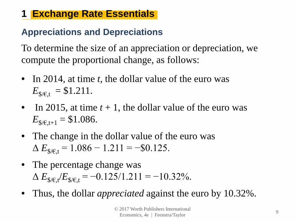
1 Exchange Rate Essentials
Appreciations and Depreciations
To determine the size of an appreciation or depreciation, we compute the proportional change, as follows:
• In 2014, at time t, the dollar value of the euro was E$/€,t = $1.211.
• In 2015, at time t + 1, the dollar value of the euro was E$/€,t+1 = $1.086.
• The change in the dollar value of the euro wasΔ E$/€,t = 1.086 − 1.211 = −$0.125.
• The percentage change was Δ E$/€,t/E$/€,t = −0.125/1.211 = −10.32%.
• Thus, the dollar appreciated against the euro by 10.32%.
© 2017 Worth Publishers International Economics, 4e | Feenstra/Taylor
9

1 Exchange Rate Essentials
Appreciations and Depreciations
Similarly, over the same year:
• In 2014, at time t, the euro value of the dollar was E€ /$,t = €0.826.
• In 2015, at time t + 1, the euro value of the dollar wasE€ /$,t+1 = €0.921.
• The change in the dollar value of the euro was ΔE€ /$,t = 0.921 − 0.826 = +€0.095.
• The percentage change was ΔE€/$,t / E€/$,t = +0.095/0.826 = +11.50%.
• Thus, the euro depreciated against the dollar by 11.50%.
© 2017 Worth Publishers International Economics, 4e | Feenstra/Taylor
10

1 Exchange Rate Essentials
Multilateral Exchange Rates
Economists calculate multilateral exchange rate changes by aggregating bilateral exchange rates using trade weights to construct an average over each currency in the basket. The resulting measure is called the change in the effective exchange rate. For example:
• Suppose 40% of Home trade is with country 1 and 60% is with country 2. Home’s currency appreciates 10% against 1 but depreciates 30% against 2.
• To find the change in Home’s effective exchange rate, multiply each exchange rate change by the trade share and sum:
(−10% • 40%) + (30% • 60%) = (−0.1 • 0.4) + (0.3 • 0.6) =
−0.04 + 0.18 = 0.14 = +14%.
• Home’s effective exchange rate has depreciated by 14%.© 2017 Worth Publishers International
Economics, 4e | Feenstra/Taylor11

1 Exchange Rate Essentials
Multilateral Exchange Rates
In general, suppose there are N currencies in the basket, and Home’s trade with all N partners is:
Trade = Trade1 + Trade2 + . . . + TradeN.
Applying trade weights to each bilateral exchange rate change, the home country’s effective exchange rate (Eeffective) will change according to the following weighted average:
���������
���������
�
�
� �
�
� �
�
�
�������������� ������� �� ��������� ������� �������� ���� �������
© 2017 Worth Publishers International Economics, 4e | Feenstra/Taylor
12

1 Exchange Rate Essentials
Multilateral Exchange Rates
FIGURE 2-1
Effective Exchange Rates: Change in the Value of the U.S. Dollar, 2002–2015 The chart shows the value of the dollar using two different baskets of foreign currencies. Against a basket of 7 major currencies, the dollar had depreciated by 35% by early 2008. Against a broad basket of 26 currencies, the dollar had lost only 25% by 2008. This is because the dollar was floating against the major currencies, but the broad basket included important U.S. trading partners (such as China) that maintained fixed or tightly managed exchange rates against the dollar. These trends only briefly reversed during the global financial crisis of 2008 before continuing up to 2015.
© 2017 Worth Publishers International Economics, 4e | Feenstra/Taylor
13

1 Exchange Rate Essentials
Example: Using Exchange Rates to Compare Prices in a Common Currency
TABLE 2-2
Using the Exchange Rate to Compare Prices in a Common Currency Now pay attention, 007! This table shows how the hypothetical cost of James Bond’s next tuxedo in different locations depends on the exchange rates that prevail.
© 2017 Worth Publishers International Economics, 4e | Feenstra/Taylor
14
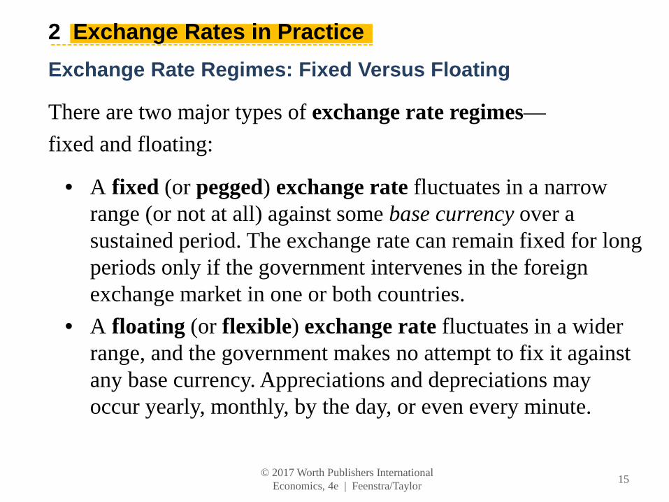
2 Exchange Rates in Practice
Exchange Rate Regimes: Fixed Versus Floating
There are two major types of exchange rate regimes—
fixed and floating:
• A fixed (or pegged) exchange rate fluctuates in a narrow range (or not at all) against some base currency over a sustained period. The exchange rate can remain fixed for long periods only if the government intervenes in the foreign exchange market in one or both countries.
• A floating (or flexible) exchange rate fluctuates in a wider range, and the government makes no attempt to fix it against any base currency. Appreciations and depreciations may occur yearly, monthly, by the day, or even every minute.
© 2017 Worth Publishers International Economics, 4e | Feenstra/Taylor
15

APPLICATION
FIGURE 2-2 (1 of 2) Exchange Rate Behavior: Selected Developed Countries, 1996–2015
This figure shows the exchange rates of three currencies against the U.S. dollar. The U.S. dollar is in a floating relationship with the yen, the pound, and the Canadian dollar (or loonie). The U.S. dollar is subject to a great deal of volatility because it is in a floating regime, or free float.
© 2017 Worth Publishers International Economics, 4e | Feenstra/Taylor
16

APPLICATION
FIGURE 2-2 (2 of 2) Exchange Rate Behavior: Selected Developed Countries, 1996–2015 (cont.)
This figure shows exchange rates of three currencies against the euro, which was introduced in 1999. The pound and the yen float against the euro. The Danish krone provides an example of a fixed exchange rate. There is only a tiny variation around this rate, no more than plus or minus 2%. This type of fixed regime is known as a band.
© 2017 Worth Publishers International Economics, 4e | Feenstra/Taylor
17

APPLICATION
FIGURE 2-3 (1 of 2) Exchange Rate Behavior: Selected Developing Countries, 1996–2015
Selected Developing Countries, 1996–2015 Exchange rates in developing countries show a wide variety of experiences and greater volatility. Pegging is common but is punctuated by periodic crises (you can see the effects of these crises in graphs for Thailand, South Korea, and India).
© 2017 Worth Publishers International Economics, 4e | Feenstra/Taylor
18

APPLICATION
FIGURE 2-3 (2 of 2) Exchange Rate Behavior: Selected Developing Countries, 1996–2015 (cont.)
India is an example of a middle ground, somewhere between a fixed rate and a free float, called a managed float. Colombia is an example of a crawling peg. The Colombian peso is allowed to crawl gradually, and it steadily depreciated at an almost constant rate for several years from 1996 to 2002. Dollarization occurred in Ecuador in 2000, a process that occurs when a country unilaterally adopts the currency of another country.
© 2017 Worth Publishers International Economics, 4e | Feenstra/Taylor
19

APPLICATION
Recent Exchange Rate Experiences
Exchange Rate Regimes of the World
• Figure 2-4 shows an IMF classification of exchange rate regimes around the world, which allows us to see the prevalence of different regime types across the whole spectrum, from fixed to floating.
• The classification covers 182 economies for the year 2010, and regimes are ordered from the most rigidly fixed to the most freely floating.
• Six of these countries have a currency board, a type of fixed regime that has special legal and procedural rules designed to make the peg “harder”—that is, more durable.
© 2017 Worth Publishers International Economics, 4e | Feenstra/Taylor
20

APPLICATION
FIGURE 2-4 A Spectrum of Exchange Rate Regimes
This figure shows IMF classification of exchange rate regimes around the world for 182 economies in 2010. Regimes are ordered from the most rigidly fixed to the most freely floating. Six countries use an ultra-hard peg called a currency board, while 35 others have a hard peg.
© 2017 Worth Publishers International Economics, 4e | Feenstra/Taylor
21

APPLICATION
FIGURE 2-4) A Spectrum of Exchange Rate Regimes (continued)
An additional 43 counties have bands, crawling pegs, or crawling bands, while 46 countries have exchange rates that either float freely, are managed floats, or are allowed to float within wide bands.
© 2017 Worth Publishers International Economics, 4e | Feenstra/Taylor
22

3 The Market for Foreign Exchange
Exchange rates the world over are set in the foreign exchange market (or forex or FX market).
• The forex market is not an organized exchange: Trade is conducted “over the counter.”
• In January 2013, the global forex market traded $5.3 trillion per day in currency.
• The three major foreign exchange centers are located in the United Kingdom, the United States, and Japan.
• Other important centers for forex trade include Hong Kong, Paris, Singapore, Sydney, and Zurich.
© 2017 Worth Publishers International Economics, 4e | Feenstra/Taylor
23

3 The Market for Foreign Exchange
The Spot Contract
• The simplest forex transaction is a contract for the immediate exchange of one currency for another between two parties. This is known as a spot contract.
• The exchange rate for this transaction is often called the spot exchange rate.
• The use of the term “exchange rate” always refers to the spot rate for our purposes.
• The spot contract is the most common type of trade and appears in almost 90% of all forex transactions.
© 2017 Worth Publishers International Economics, 4e | Feenstra/Taylor
24

3 The Market for Foreign Exchange
Derivatives
• In addition to the spot contracts other forex contracts include forwards, swaps, futures, and options.
• Collectively, all these related forex contracts are termed derivatives.
• The spot and forward rates closely track each other.
FIGURE 2-5
© 2017 Worth Publishers International Economics, 4e | Feenstra/Taylor
25

APPLICATION
Foreign Exchange Derivatives
Forwards
A forward contract differs from a spot contract in that the two parties make the contract today, but the settlement date for the delivery of the currencies is in the future, or forward. The time to delivery, or maturity, varies. However, because the price is fixed as of today, the contract carries no risk.
Swaps
A swap contract combines a spot sale of foreign currency with a forward repurchase of the same currency. This is a common contract for counterparties dealing in the same currency pair over and over again. Combining two transactions reduces transactions costs.
© 2017 Worth Publishers International Economics, 4e | Feenstra/Taylor
26

APPLICATION
Foreign Exchange Derivatives
Futures
A futures contract is a promise that the two parties holding the contract will deliver currencies to each other at some future date at a prespecified exchange rate, just like a forward contract. Unlike the forward contract, futures contracts are standardized, mature at certain regular dates, and can be traded on an organized futures exchange.
Options
An option provides one party, the buyer, with the right to buy (call) or sell (put) a currency in exchange for another at a prespecified exchange rate at a future date. The buyer is under no obligation to trade and will not exercise the option if the spot price on the expiration date turns out to be more favorable.
© 2017 Worth Publishers International Economics, 4e | Feenstra/Taylor
27

APPLICATION
Foreign Exchange Derivatives
Derivatives allow investors to engage in hedging (risk avoidance) and speculation (risk taking).
• Example 1: Hedging. As chief financial officer of a U.S. firm, you expect to receive payment of €1 million in 90 days for exports to France. The current spot rate is $1.20 per euro. Your firm will incur losses on the deal if the euro weakens to less than $1.10 per euro. You advise that the firm buy €1 million in call options on dollars at a rate of $1.15 per euro, ensuring that the firm’s euro receipts will sell for at least this rate. This locks in a minimal profit even if the spot rate falls below $1.15. This is hedging.
© 2017 Worth Publishers International Economics, 4e | Feenstra/Taylor
28

APPLICATION
Foreign Exchange Derivatives
Derivatives allow investors to engage in hedging (risk avoidance) and speculation (risk taking).
• Example 2: Speculation. The market currently prices one-year euro futures at $1.30, but you think the dollar will weaken to $1.43 in the next 12 months. If you wish to make a bet, you would buy these futures, and if you are proved right, you will realize a 10% profit. Any level above $1.30 will generate a profit. If the dollar is at or below $1.30 a year from now, however, your investment in futures will be a total loss. This is speculation.
© 2017 Worth Publishers International Economics, 4e | Feenstra/Taylor
29

3 The Market for Foreign Exchange
Private Actors
• Most forex traders work for commercial banks. About 75% of all forex transactions globally are handled by just 10 banks.
• The exchange rates for these trades underlie quoted market exchange rates.
• Some corporations may trade in the market if they are engaged in extensive transactions in foreign markets.
Government Actions
• Some governments engage in policies that restrict trading, movement of forex, or cross-border financial transactions. These are called a form of capital control.
• In lieu of capital controls, the central bank must stand ready to buy or sell its own currency to maintain a fixed exchange rate.
© 2017 Worth Publishers International Economics, 4e | Feenstra/Taylor
30

4 Arbitrage and Spot Exchange Rates
FIGURE 2-6
Arbitrage and Spot Rates Arbitrage ensures that the trade of currencies in New York along the path AB occurs at the same exchange rate as via London along path ACDB. At B the pounds received must be the same, regardless of the route taken to get to B:
£/$�.�.
£/$������
© 2017 Worth Publishers International Economics, 4e | Feenstra/Taylor
31

4 Arbitrage and Spot Exchange Rates
Arbitrage with Three Currencies
In general, three outcomes are again possible.
1. The direct trade from dollars to pounds has a better rate: E£/$ > E£/€ E€/$
2. The indirect trade has a better rate: E£/$ < E£/€ E€/$
3. The two trades have the same rate and yield the same result: E£/$ = E£/€ E€/$. Only in the last case are there no profit opportunities. This is the no-arbitrage condition:
The right-hand expression, a ratio of two exchange rates, is called a cross rate. © 2017 Worth Publishers International
Economics, 4e | Feenstra/Taylor32
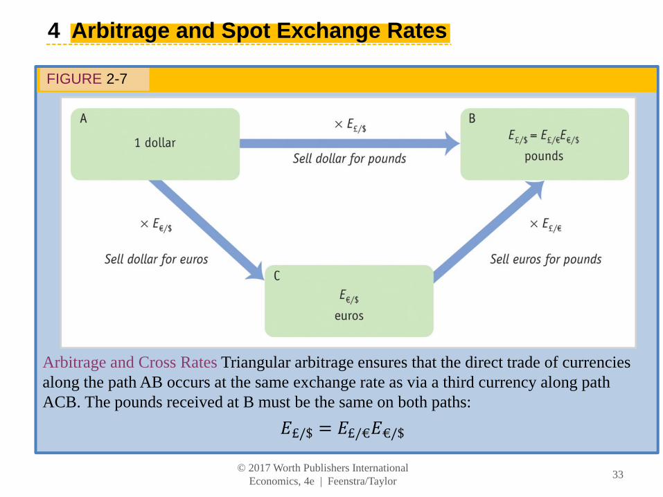
4 Arbitrage and Spot Exchange Rates
FIGURE 2-7
Arbitrage and Cross Rates Triangular arbitrage ensures that the direct trade of currencies along the path AB occurs at the same exchange rate as via a third currency along path ACB. The pounds received at B must be the same on both paths:
© 2017 Worth Publishers International Economics, 4e | Feenstra/Taylor
33
£/$ £/€ €/$
4 Arbitrage and Spot Exchange Rates
Cross Rates and Vehicle Currencies
• The majority of the world’s currencies trade directly with only one or two of the major currencies, such as the dollar, euro, yen, or pound.
• Many countries do a lot of business in major currencies such as the U.S. dollar, so individuals always have the option to engage in a triangular trade at the cross rate.
• When a third currency, such as the U.S. dollar, is used in these transactions, it is called a vehicle currency because it is not the home currency of either of the parties involved in the trade and is just used for intermediation.
© 2017 Worth Publishers International Economics, 4e | Feenstra/Taylor
34

5 Arbitrage and Interest Rates
An important question for investors is in which currency they should hold their liquid cash balances.
• Would selling euro deposits and buying dollar deposits make a profit for a banker?
• These decisions drive demand for dollars versus euros and the exchange rate between the two currencies.
The Problem of Risk
A trader in New York cares about returns in U.S. dollars. A dollar deposit pays a known return, in dollars. But a euro deposit pays a return in euros, and one year from now we cannot know for sure what the dollar–euro exchange rate will be.
• Riskless arbitrage and risky arbitrage lead to two important implications, called parity conditions.
© 2017 Worth Publishers International Economics, 4e | Feenstra/Taylor
35

5 Arbitrage and Interest Rates
Riskless Arbitrage: Covered Interest Parity
Contracts to exchange euros for dollars in one year’s time carry an exchange rate of F$/€ dollars per euro. This is known as the forward exchange rate.
• If you invest in a dollar deposit, your $1 placed in a U.S. bank account will be worth (1 + i$) dollars in one year’s time. The dollar value of principal and interest for the U.S. dollar bank deposit is called the dollar return.
• If you invest in a euro deposit, you first need to convert the dollar to euros. Using the spot exchange rate, $1 buys 1/E$/€
euros today.
• These 1/E$/€ euros would be placed in a euro account earning i€, so in a year’s time they would be worth (1 + i€)/E$/€ euros.
© 2017 Worth Publishers International Economics, 4e | Feenstra/Taylor
36

5 Arbitrage and Interest Rates
Riskless Arbitrage: Covered Interest Parity
To avoid that risk, you engage in a forward contract today to make the future transaction at a forward rate F$/€.
• The (1 + i€)/E$/€ euros you will have in one year’s time can then be exchanged for (1 + i€)F$/€/E$/€ dollars, or the dollar return on the euro bank deposit.
$/€
$/€
• This is called covered interest parity (CIP) because all exchange rate risk on the euro side has been “covered” by use of the forward contract.
© 2017 Worth Publishers International Economics, 4e | Feenstra/Taylor
37

5 Arbitrage and Interest Rates
FIGURE 2-8
Arbitrage and Covered Interest Parity Under CIP, returns to holding dollar deposits accruing interest going along the path AB must equal the returns from investing in euros going along the path ACDB with risk removed by use of a forward contract. Hence, at B, the riskless payoff must be the same on both paths:
© 2017 Worth Publishers International Economics, 4e | Feenstra/Taylor
38

APPLICATION
Evidence on Covered Interests Parity
FIGURE 2-9 (1 of 2) Financial Liberalization and Covered Interest Parity
Financial Liberalization and Covered Interest Parity: Arbitrage Between the United Kingdom and Germany The chart shows the difference in monthly pound returns on deposits in British pounds and German marks using forward cover from 1970 to 1995. In the 1970s, the difference was positive and often large: Traders would have profited from arbitrage by moving money from pound deposits to mark deposits, but capital controls prevented them from freely doing so.
© 2017 Worth Publishers International Economics, 4e | Feenstra/Taylor
39

APPLICATION
Evidence on Covered Interest Parity
FIGURE 2-9 (2 of 2) Financial Liberalization and Covered Interest Parity (continued)
After financial liberalization, these profits essentially vanished, and no arbitrage opportunities remained. The CIP condition held, aside from small deviations resulting from transactions costs and measurement errors.
© 2017 Worth Publishers International Economics, 4e | Feenstra/Taylor
40

5 Arbitrage and Interest Rates
Risky Arbitrage: Uncovered Interest Parity
• In this case, traders face exchange rate risk and must make a forecast of the future spot rate. We refer to the forecast as
, which we call the expected exchange rate.
• Based on the forecast, you expect that the euros you will have in one year’s time will be worth when converted into dollars; this is the expected dollar returnon euro deposits.
• The expression for uncovered interest parity (UIP) is:
$/€�
€ $/€
€ $/€�
$/€
© 2017 Worth Publishers International Economics, 4e | Feenstra/Taylor
41

5 Arbitrage and Interest Rates
FIGURE 2-10
Arbitrage and Uncovered Interest Parity Under CIP, returns to holding dollar deposits accruing interest going along the path AB must equal returns from investing in euros going along the risky path ACDB. Hence, at B, the expected payoff must be the same on both paths:
$$/€�
$/€€
© 2017 Worth Publishers International Economics, 4e | Feenstra/Taylor
42

5 Arbitrage and Interest Rates
Risky Arbitrage : Uncovered Interest Parity
What Determines the Spot Rate?
• Uncovered interest parity is a no-arbitrage condition that describes an equilibrium in which investors are indifferent between the returns on unhedged interest-bearing bank deposits in two currencies.
• We can rearrange the terms in the uncovered interest parity expression to solve for the spot rate:
© 2017 Worth Publishers International Economics, 4e | Feenstra/Taylor
43

Assets and Their Attributes
• An investor’s entire portfolio of assets may include stocks, bonds, real estate, art, bank deposits in various currencies, and so on. All assets have three key attributes that influence demand: return, risk, and liquidity.
• An asset’s rate of return is the total net increase in wealth resulting from holding the asset for a specified period of time, typically one year.
• The risk of an asset refers to the volatility of its rate of return.
• The liquidity of an asset refers to the ease and speed with which it can be liquidated, or sold.
• We refer to the forecast of the rate of return as the expected rate of return.
© 2017 Worth Publishers International Economics, 4e | Feenstra/Taylor
44

APPLICATION
Evidence on Uncovered Interest Parity
• Dividing the UIP by the CIP, we obtain $/€�
$/€ , or
• Although the expected future spot rate and the forward rate are used in two different forms of arbitrage—risky and riskless, in equilibrium they should be exactly the same!
• If both covered interest parity and uncovered interest parity hold, the forward must equal the expected future spot rate.
• Risk-neutral investors have no reason to prefer to avoid risk by using the forward rate versus embracing risk by awaiting the future spot rate.
© 2017 Worth Publishers International Economics, 4e | Feenstra/Taylor
45

APPLICATION
Evidence on Uncovered Interest Parity
• If the forward rate equals the expected spot rate, the expected rate of depreciation equals the forward premium (the proportional difference between the forward and spot rates):
• While the left-hand side is easily observed, the expectations on the right-hand side are typically unobserved.
© 2017 Worth Publishers International Economics, 4e | Feenstra/Taylor
46

APPLICATION
Evidence on Uncovered Interest Parity
FIGURE 2-11
Evidence on Interest Parity
When UIP and CIP hold, the 12-month forward premium should equal the 12-month expected rate of depreciation. A scatterplot showing these two variables should be close to the diagonal 45-degree line.
Using evidence from surveys of individual forex traders’ expectations over the period 1988 to 1993, UIP finds some support, as the line of best fit is close to the diagonal.
© 2017 Worth Publishers International Economics, 4e | Feenstra/Taylor
47

5 Arbitrage and Interest Rates
Uncovered Interest Parity: A Useful Approximation
$
�������������� ������ ��������
������� ���� �� �������� ������ ��������
€
�������������� ���� ��������
$/€�
$/€
�������� ���� �� �������������� ��� ������
�������� ������ ���� �� �������� ���� ��������
• This approximate equation for UIP says that the home interest rate equals the foreign interest rate plus the expected rate of depreciation of the home currency.
• Suppose the dollar interest rate is 4% per year and the euro 3%. If UIP is to hold, the expected rate of dollar depreciation over a year must be 1%. The total dollar return on the euro deposit is approximately equal to the 4% that is offered by dollar deposits.
© 2017 Worth Publishers International Economics, 4e | Feenstra/Taylor
48

5 Arbitrage and Interest Rates
Summary
FIGURE 2-12
How Interest Parity Relationships Explain Spot and Forward Rates In the spot market, UIP provides a model of how the spot exchange rate is determined. To use UIP to find the spot rate, we need to know the expected future spot rate and the prevailing interest rates for the two currencies. In the forward market, CIP provides a model of how the forward exchange rate is determined. When we use CIP, we derive the forward rate from the current spot rate (from UIP) and the interest rates for the two currencies.
© 2017 Worth Publishers International Economics, 4e | Feenstra/Taylor
49

KEY POINTS
1. The exchange rate in a country is the price of a unit of foreign currency expressed in terms of the home currency. This price is determined in the spot market for foreign exchange.
© 2017 Worth Publishers International Economics, 4e | Feenstra/Taylor
50

2. When the home exchange rate rises, less foreign currency is bought/sold per unit of home currency; the home currency has depreciated. If home currency buys x% less foreign currency, the home currency is said to have depreciated by x%.
KEY POINTS
© 2017 Worth Publishers International Economics, 4e | Feenstra/Taylor
51

KEY POINTS
3. When the home exchange rate falls, more foreign currency is bought/sold per unit of home currency; the home currency has appreciated. If home currency buys x% more foreign currency, the home currency is said to have appreciated by x%.
© 2017 Worth Publishers International Economics, 4e | Feenstra/Taylor
52

KEY POINTS
4. The exchange rate is used to convert the prices of goods and assets into a common currency to allow meaningful price comparisons.
© 2017 Worth Publishers International Economics, 4e | Feenstra/Taylor
53

KEY POINTS
5. Exchange rates may be stable over time or they may fluctuate. History supplies examples of the former (fixed exchange rate regimes) and the latter (floating exchange rate regimes) as well as a number of intermediate regime types.
© 2017 Worth Publishers International Economics, 4e | Feenstra/Taylor
54

KEY POINTS
6. An exchange rate crisis occurs when the exchange rate experiences a sudden and large depreciation. These events are often associated with broader economic and political turmoil, especially in developing countries.
© 2017 Worth Publishers International Economics, 4e | Feenstra/Taylor
55

KEY POINTS
7. Some countries may forgo a national currency to form a currency union with other nations (e.g., the Eurozone), or they may unilaterally adopt the currency of another country (“dollarization”).
© 2017 Worth Publishers International Economics, 4e | Feenstra/Taylor
56

KEY POINTS
8. Looking across all countries today, numerous fixed and floating rate regimes are observed, so we must understand both types of regime.
© 2017 Worth Publishers International Economics, 4e | Feenstra/Taylor
57

KEY POINTS
9. The forex market is dominated by spot transactions, but many derivative contracts exist, such as forwards, swaps, futures, and options.
© 2017 Worth Publishers International Economics, 4e | Feenstra/Taylor
58

KEY POINTS
10. The main actors in the market are private investors and (frequently) government authorities, usually represented by the central bank.
© 2017 Worth Publishers International Economics, 4e | Feenstra/Taylor
59

KEY POINTS
11. Arbitrage on currencies means that spot exchange rates are approximately equal in different forex markets. Cross rates (for indirect trades) and spot rates (for direct trades) are also approximately equal.
© 2017 Worth Publishers International Economics, 4e | Feenstra/Taylor
60

KEY POINTS
12. Riskless interest arbitrage leads to the covered interest parity (CIP) condition. CIP says that the dollar return on dollar deposits must equal the dollar return on euro deposits, where forward contracts are used to cover exchange rate risk.
© 2017 Worth Publishers International Economics, 4e | Feenstra/Taylor
61

KEY POINTS
13. Covered interest parity says that the forward rate is determined by home and foreign interest rates and the spot exchange rate.
© 2017 Worth Publishers International Economics, 4e | Feenstra/Taylor
62

KEY POINTS
14. Risky interest arbitrage leads to the uncovered interest parity (UIP) condition. UIP says that when spot contracts are used and exchange rate risk is not covered, the dollar return on dollar deposits must equal the expected dollar returns on euro deposits.
© 2017 Worth Publishers International Economics, 4e | Feenstra/Taylor
63
KEY POINTS
15. Uncovered interest parity explains how the spot rate is determined by the home and foreign interest rates and the expected future spot exchange rate.
© 2017 Worth Publishers International Economics, 4e | Feenstra/Taylor
64

KEY TERMSexchange rate
appreciation
depreciation
effective exchange rate
exchange rate regimes
fixed (or pegged) exchangerates
floating (or flexible) exchangerates
free float exchange rate regime
band
managed float
exchange rate crises
crawling peg
currency (or monetary) union
dollarization
currency board
foreign exchange (forex or FX)market
spot contract
spot exchange rate
spread
market friction
transaction costs
derivatives
forward
swap
futures
option
commercial banks
interbank trading
corporations
nonbank financialinstitutions
capital control
official market
black market
intervention
arbitrage
equilibrium
no-arbitrage condition
cross rate
vehicle currency
forward exchange rate
covered interest parity (CIP)
rate of return
risk
liquidity
expected rate of return
expected exchange rate
uncovered interest parity(UIP)
expected rate ofdepreciation
forward premium
© 2017 Worth Publishers International Economics, 4e | Feenstra/Taylor
65
Trade and Technology: The Ricardian ModelQuestions to Consider
1. What are reasons for countries to trade?
2. Will the country that is best at producing a good always export it?
3. How can countries compete with low-wage exporters, like China?
© 2017 Worth Publishers International Economics, 4e | Feenstra/Taylor
1

Introduction
Where did Jamie Anderson’s snowboard come from?
• In 2014 the United States imported(i.e., purchased from other countries) $28 million of snowboards from 18 different countries.
• China exported (i.e., sold to another country) nearly $13 million worth of snowboards to the United States in 2014.
Doug Pensinger/Getty Images
© 2017 Worth Publishers International Economics, 4e | Feenstra/Taylor
2

Introduction
TABLE 2-1 U.S. Imports of Snowboards, 2014
Table 2-1 shows that the U.S. imported 350,600 snowboards from 18 countries in 2014 that were worth more than $28 million.
This pattern raises a question: With all the manufacturing capability in the United States, why does it purchase snowboards from these countries at all instead of producing them domestically?
© 2017 Worth Publishers International Economics, 4e | Feenstra/Taylor
3

Introduction
In this chapter, we will:
• Learn the reasons countries trade
• Distinguish between absolute and comparative advantage
• Understand the Ricardian model
• Understand the no-trade equilibrium using each country’s PPF and indifference curve
• Solve for wages across countries
• Solve for international prices
• Derive the home export supply and Foreign import demand curve and how to arrive at international trade equilibrium © 2017 Worth Publishers International
Economics, 4e | Feenstra/Taylor4

Introduction
Reasons countries trade goods with each other
• Differences in the technology used in each country (i.e., differences in each country’s ability to manufacture products)
• Differences in the total amount of resources (including labor, capital, and land) found in each country
• Differences in the costs of offshoring (i.e., producing the various parts of a good in different countries and then assembling it in a final location)
• The proximity of countries to each other (i.e., how close they are to one another)
© 2017 Worth Publishers International Economics, 4e | Feenstra/Taylor
5

Introduction
In this chapter, we focus on technology differences across countries as an explanation for trade, called the Ricardian model.
• The Ricardian model explains how the level of a country’s technology affects its trade pattern.
• It also explains the concept of comparative advantage and why it works as an explanation for trade patterns.
© 2017 Worth Publishers International Economics, 4e | Feenstra/Taylor
6

1 Reasons for Trade
Proximity
• The closer countries are, the lower the costs of transportation. For example, the largest trading partner of most European countries is another European country.
Resources
• Geography includes natural resources, as well as labor resources and capital. A country’s resources are often collectively called its factors of production, the land, labor, and capital used to produce goods and services.
© 2017 Worth Publishers International Economics, 4e | Feenstra/Taylor
7

1 Reasons for Trade
Absolute Advantage
• When a country has the best technology for producing a good, it has an absolute advantage in the production of that good.
• Absolute advantage is not a good explanation for trade patterns.
Comparative Advantage
• Instead, comparative advantage is the primary explanation for trade among countries.
• A country has comparative advantage in producing those goods that it produces best compared with how well it produces other goods.
© 2017 Worth Publishers International Economics, 4e | Feenstra/Taylor
8
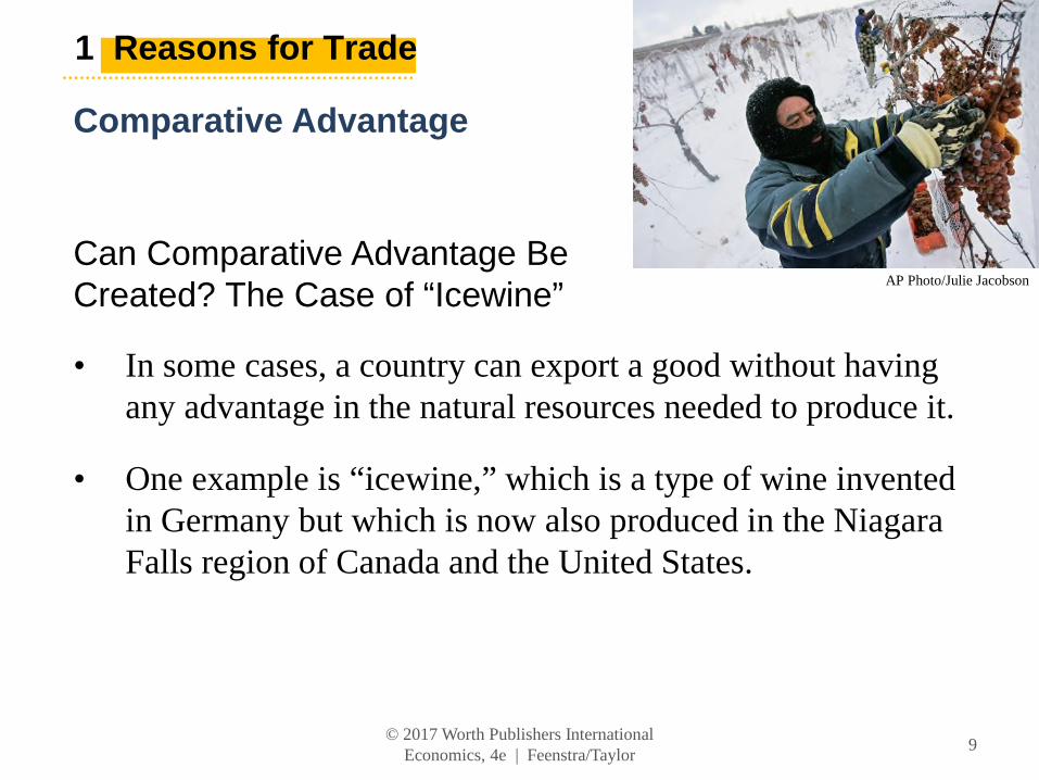
1 Reasons for Trade
Comparative Advantage
Can Comparative Advantage BeCreated? The Case of “Icewine”
• In some cases, a country can export a good without having any advantage in the natural resources needed to produce it.
• One example is “icewine,” which is a type of wine invented in Germany but which is now also produced in the Niagara Falls region of Canada and the United States.
AP Photo/Julie Jacobson
© 2017 Worth Publishers International Economics, 4e | Feenstra/Taylor
9

David Ricardo and Mercantilism
• Mercantilists believed that exporting was goodbecause it generated gold and importing was bad because it drained gold from the national treasury.
• Mercantilists were in favor of high tariffs to ensure high exports and low imports.
• Ricardo showed that countries could benefit from international trade without having to use tariffs.
• Many of today’s major international institutions around the world were founded at least in part on the idea that free trade between countries brings gains for all trading partners.
Bettman/Corbis
© 2017 Worth Publishers International Economics, 4e | Feenstra/Taylor
10

2 Ricardian Model
The Home Country
To develop a Ricardian model of trade, we will use an example with two goods:
• Wheat and other grains are major exports of the United States and Europe.
• Many types of cloth are imported into these countries.
For simplicity, we ignore the role of land and capital and suppose that both goods are produced with labor alone.
© 2017 Worth Publishers International Economics, 4e | Feenstra/Taylor
11

2 Ricardian Model
The Home Country
We assume that labor is the only resource used to produce goods. The marginal product of labor (MPL) is the extra output obtained by using one more unit of labor.
• In Home, one worker produces 4 bushels of wheat, so MPLW = 4.
• Alternatively, one worker can produce 2 yards of cloth, so MPLC = 2.
© 2017 Worth Publishers International Economics, 4e | Feenstra/Taylor
12

2 Ricardian Model
The Home Country
Home Production Possibilities Frontier
• We can graph Home’s production possibilities frontier (PPF) using the marginal products for wheat and cloth.
• The slope of the PPF is also the opportunity cost of wheat, the amount of cloth that must be given up to obtain one more unit of wheat.
• If Home had 25 workers and all were employed in wheat, Home could produce 100 bushels. If all were employed in cloth, they could produce 50 yards.
© 2017 Worth Publishers International Economics, 4e | Feenstra/Taylor
13

2 Ricardian Model
The Home Country
Home Production Possibilities FrontierFIGURE 2-1
The Home PPF is a straight line between 50 yards of cloth and 100 bushels of wheat.
The slope of the PPF equals the negative of the opportunity cost of wheat. Equivalently, the magnitude of the slope can be expressed as the ratio of the marginal products of labor for the two goods.
�
�
�
�© 2017 Worth Publishers International
Economics, 4e | Feenstra/Taylor14

2 Ricardian Model
The Home Country
Home Indifference Curve
We will represent demand in the Home economy using indifference curves that have the following properties:
• All points on an indifference curve have the same level of utility.
• Points on higher indifference curves have higher utility.
• Each indifference curve shows the combinations of two goods, such as wheat and cloth, that a person or economy can consume and be equally satisfied.
© 2017 Worth Publishers International Economics, 4e | Feenstra/Taylor
15

2 Ricardian Model
Home Indifference Curve
FIGURE 2-2 Home Equilibrium with No Trade
Points A and B lie on the same indifference curve and give the Home consumers the level of utility U1.
The highest level of Home utility on the PPF is obtained at point A, which is the no-trade equilibrium.
Point D is also on the PPF but would give lower utility.
Point C represents a higher utility level but is off of the PPF, so it is not attainable in the absence of international trade.
© 2017 Worth Publishers International Economics, 4e | Feenstra/Taylor
16

2 Ricardian Model
The Home Country
Opportunity Cost and Prices
• The slope of the PPF reflects the opportunity cost of producing one more bushel of wheat.
• Under perfect competition the opportunity cost of wheat should also equal the relative price of wheat.
• Price reflects the opportunity cost of a good.
© 2017 Worth Publishers International Economics, 4e | Feenstra/Taylor
17

2 Ricardian Model
The Home Country
Wages
• In competitive markets firms hire workers up to the point at which the hourly wage equals the value of one more hour of production.
• The value of one more hour of labor equals the amount of goods produced in that hour (MPL) times the price of the good.
• Labor will be hired up to the point where wage equals P • MPL for each industry.
© 2017 Worth Publishers International Economics, 4e | Feenstra/Taylor
18
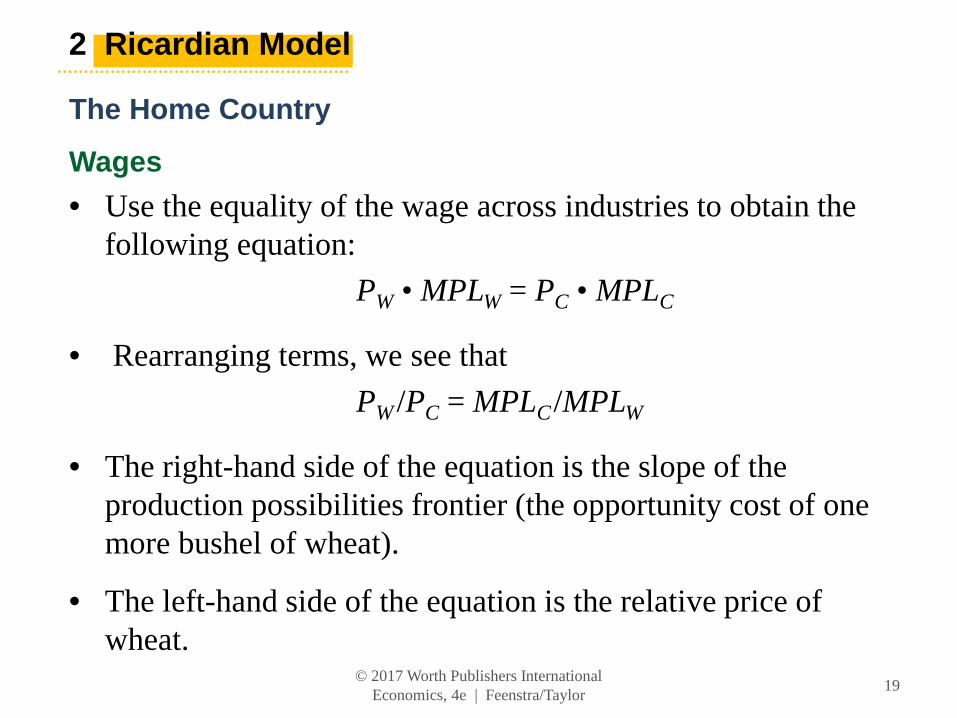
2 Ricardian Model
The Home Country
Wages
• Use the equality of the wage across industries to obtain the following equation:
PW • MPLW = PC • MPLC
• Rearranging terms, we see that
PW /PC = MPLC/MPLW
• The right-hand side of the equation is the slope of the production possibilities frontier (the opportunity cost of one more bushel of wheat).
• The left-hand side of the equation is the relative price of wheat.
© 2017 Worth Publishers International Economics, 4e | Feenstra/Taylor
19
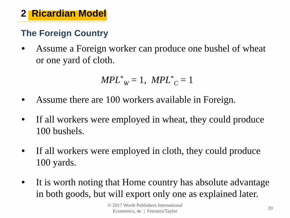
2 Ricardian Model
The Foreign Country
• Assume a Foreign worker can produce one bushel of wheat or one yard of cloth.
MPL*W = 1, MPL*
C = 1
• Assume there are 100 workers available in Foreign.
• If all workers were employed in wheat, they could produce 100 bushels.
• If all workers were employed in cloth, they could produce 100 yards.
• It is worth noting that Home country has absolute advantage in both goods, but will export only one as explained later.
© 2017 Worth Publishers International Economics, 4e | Feenstra/Taylor
20

2 Ricardian Model
The Foreign Country
Foreign Production Possibilities Frontier
FIGURE 2-3
The Foreign PPF is a straight line between 100 yards of cloth and 100 bushels of wheat.
The slope of the PPF equals the negative of the opportunity cost of wheat.
The opportunity cost is the amount of cloth that must be given up (1 yard) to obtain 1 more bushel of wheat.
© 2017 Worth Publishers International Economics, 4e | Feenstra/Taylor
21

2 Ricardian Model
Comparative Advantage
• A country has a comparative advantage in a good when it has a lower opportunity cost of producing than another country.
• By looking at the chart we can see that Foreign has a comparative advantage in producing cloth. Home has a comparative advantage in producing wheat.
© 2017 Worth Publishers International Economics, 4e | Feenstra/Taylor
22
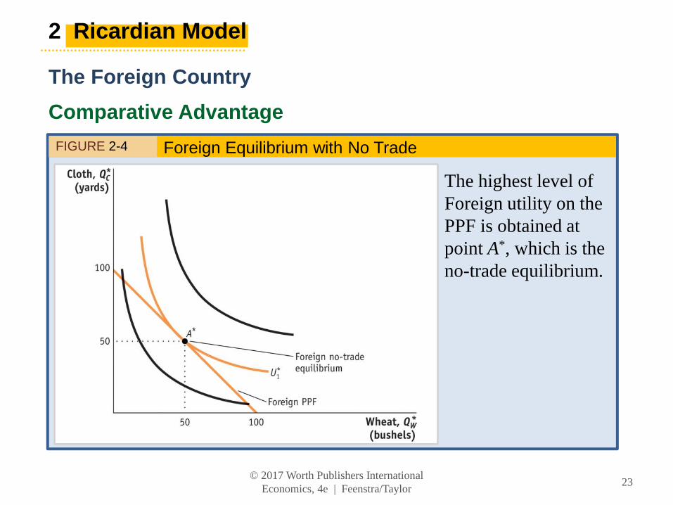
2 Ricardian Model
The Foreign Country
Comparative Advantage
FIGURE 2-4 Foreign Equilibrium with No Trade
The highest level of Foreign utility on the PPF is obtained at point A*, which is the no-trade equilibrium.
© 2017 Worth Publishers International Economics, 4e | Feenstra/Taylor
23

APPLICATIONS
Comparative Advantage in Apparel, Textiles, and Wheat
TABLE 2-2 Apparel, Textiles, and Wheat in the United States and China
This table presents sales per employee for the apparel and textile industries in the United States and China, as well as bushels per hour in producing wheat. The United States has an absolute advantage in all of these products, but it has a comparative advantage in producing wheat.
© 2017 Worth Publishers International Economics, 4e | Feenstra/Taylor
24
3 Determining the Pattern of International Trade
International Trade Equilibrium
What happens when goods are traded between Home and Foreign? We will see:
• That a country’s no-trade relative price determines which product it will export and which it will import
• The no-trade relative price equals its opportunity cost of production
• The pattern of exports and imports will be determined by the opportunity costs of production in each country—their comparative advantage
© 2017 Worth Publishers International Economics, 4e | Feenstra/Taylor
25

3 Determining the Pattern of International Trade
International Trade Equilibrium
Examining each country’s no-trade relative price, we can determine which product it will export and which it will import.
• The relative price of cloth in Foreign is PC /PW = 1.
• The relative price of cloth in Home is PC /PW = 2.
• Therefore, Foreign would want to export cloth to Home they can make it for $1 and export it for more than $1.
• Home will export wheat and Foreign will export cloth.
Both countries export the good for which they have the comparative advantage.
© 2017 Worth Publishers International Economics, 4e | Feenstra/Taylor
26

3 Determining the Pattern of International Trade
International Trade Equilibrium
The two countries are in an international trade equilibrium when the relative price of wheat is the same in the two countries.
To fully understand the international trade equilibrium, we are interested in two issues:
• Determining the relative price of wheat (or cloth) in the trade equilibrium
• Seeing how the shift from the no-trade equilibrium to the trade equilibrium affects production and consumption in both Home and Foreign.
© 2017 Worth Publishers International Economics, 4e | Feenstra/Taylor
27

3 Determining the Pattern of International Trade
International Trade Equilibrium
• The relative price of wheat in the trade equilibrium will be between the no-trade price in the two countries.
• For now assume the free-trade price of PW /PC is (between
the price of in Home and 1 in Foreign).
• We can now take this price and see how trade changes production and consumption in each country.
• The world price line shows the range of consumption possibilities that a country can achieve by specializing in one good and engaging in international trade.
© 2017 Worth Publishers International Economics, 4e | Feenstra/Taylor
28

3 Determining the Pattern of International Trade
International Trade Equilibrium
Change in Production and Consumption
FIGURE 2-5 (1 of 3) Home Equilibrium with Trade
With a world relative price of wheat of 2/3, Home production will occur at point B.
Through international trade, Home is able to export each bushel of wheat it produces in
exchange for �
�yard of
cloth.
© 2017 Worth Publishers International Economics, 4e | Feenstra/Taylor
29
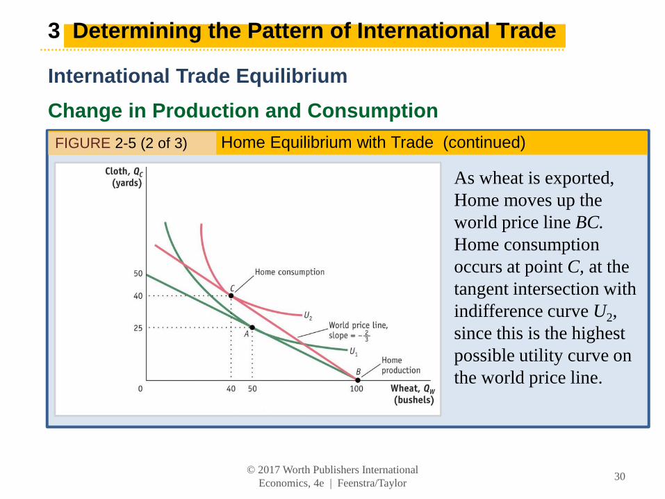
3 Determining the Pattern of International Trade
International Trade Equilibrium
Change in Production and Consumption
FIGURE 2-5 (2 of 3) Home Equilibrium with Trade (continued)
As wheat is exported, Home moves up the world price line BC. Home consumption occurs at point C, at the tangent intersection with indifference curve U2, since this is the highest possible utility curve on the world price line.
© 2017 Worth Publishers International Economics, 4e | Feenstra/Taylor
30

3 Determining the Pattern of International Trade
International Trade Equilibrium
Change in Production and Consumption
FIGURE 2-5 (3 of 3) Home Equilibrium with Trade (continued)
Given these levels of production and consumption, we can see that total exports are 60 bushels of wheat in exchange for imports of 40 yards of cloth and also that Home consumes 10 fewer bushels of wheat and 15 more yards of cloth relative to its pre-trade levels.
© 2017 Worth Publishers International Economics, 4e | Feenstra/Taylor
31

3 Determining the Pattern of International Trade
International Trade Equilibrium
FIGURE 2-5 (revisited) Home Equilibrium with Trade International Trade
Home obtains a higher utility with international trade than in the absence of trade (U2 is higher than U1).
The finding that Home’s utility increases with trade is our first demonstration of the gains from trade.
© 2017 Worth Publishers International Economics, 4e | Feenstra/Taylor
32

3 Determining the Pattern of International Trade
International Trade Equilibrium
Pattern of Trade and Gains from Trade
FIGURE 2-6 (1 of 2) Foreign Equilibrium with Trade
With a world relative price of wheat of 2/3, Foreign production will occur at point B*.
Through international trade, Foreign is able to export 2/3 yard of cloth in exchange for 1 bushel of wheat, moving down the world price line.
© 2017 Worth Publishers International Economics, 4e | Feenstra/Taylor
33

3 Determining the Pattern of International Trade
International Trade Equilibrium
Pattern of Trade and Gains from Trade
FIGURE 2-6 (2 of 2) Foreign Equilibrium with Trade (continued)
Foreign consumption occurs at point C*, and total exports are 40 yards of cloth in exchange for imports of 60 bushels of wheat. Relative to its pre-trade wheat and cloth consumption (point A*), Foreign consumes 10 more bushels of wheat and 10 more yards of cloth.
© 2017 Worth Publishers International Economics, 4e | Feenstra/Taylor
34

3 Determining the Pattern of International Trade
Pattern of Trade and Gains from Trade
Each country is exporting the good for which it has the comparative advantage.
• This confirms that the pattern of trade is determined by comparative advantage.
• This is the first lesson of the Ricardian model.
There are gains from trade for both countries.
• This is the second lesson of the Ricardian model.
© 2017 Worth Publishers International Economics, 4e | Feenstra/Taylor
35

3 Determining the Pattern of International Trade
Solving for Wages Across Countries
Home Wage =
�
���� �
�
�
�∗
�∗
�∗
�∗
Absolute Advantage
As our example shows, wages are determined by absolute
advantage. In contrast, the pattern of trade is determined by comparative advantage.
© 2017 Worth Publishers International Economics, 4e | Feenstra/Taylor
36

3 Determining the Pattern of International Trade
Solving for Wages Across Countries
• In competitive labor markets, firms will pay workers the value of their marginal product.
• Home produces and exports wheat; therefore, they will be paid in terms of that good—the real wage is MPLW = 4 bushels of wheat.
• The workers sell the wheat on the world market at a relative price of PW /PC = 2/3.
• We can use this to calculate the real wage in terms of cloth: (PW /PC)MPLW = (2/3)4 = 8/3 yards.
© 2017 Worth Publishers International Economics, 4e | Feenstra/Taylor
37

3 Determining the Pattern of International Trade
Solving for Wages Across Countries
• We can do this for Foreign as well and summarize:
Home real wage is:
• 4 bushels of wheat or 8/3 yards of cloth
Foreign real wage is:
• 3/2 bushels of wheat or 1 yard of cloth
• Foreign workers earn less than Home workers as measured by their ability to purchase either good. (The foreign real wages are still higher compare to autarky.)
• This reflects Home’s absolute advantage in the production of both goods.
© 2017 Worth Publishers International Economics, 4e | Feenstra/Taylor
38
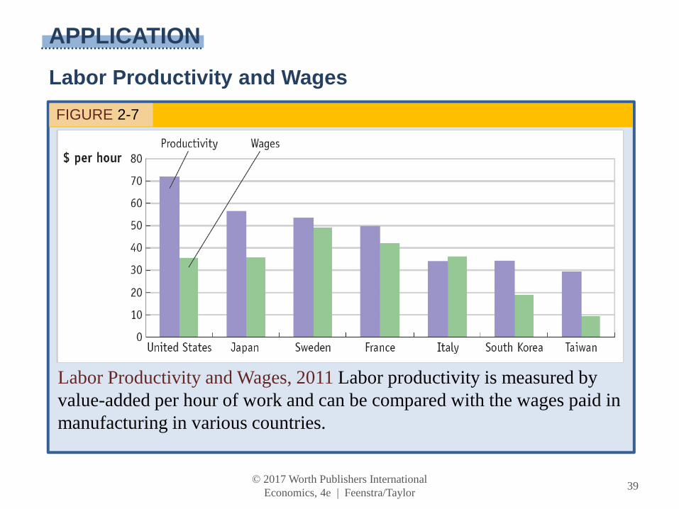
APPLICATION
Labor Productivity and Wages
FIGURE 2-7
Labor Productivity and Wages, 2011 Labor productivity is measured by value-added per hour of work and can be compared with the wages paid in manufacturing in various countries.
© 2017 Worth Publishers International Economics, 4e | Feenstra/Taylor
39

Application
Labor Productivity and Wages
FIGURE 2-8
The trends in labor productivity and wages can also be graphed over time.
The general upward movement in labor productivity is matched by upward movements in wages, as predicted by the Ricardian model.
© 2017 Worth Publishers International Economics, 4e | Feenstra/Taylor
40

4 Solving for International Prices
Home Export Supply Curve
FIGURE 2-9 (1 of 2)
Home Export Supply Panel (a) repeats Figure 2-5 showing the trade equilibrium for Home with production at point B and consumption at point C. Panel (b) shows the Home export supply of wheat.
© 2017 Worth Publishers International Economics, 4e | Feenstra/Taylor
41

4 Solving for International Prices
Home Export Supply Curve
FIGURE 2-9 (2 of 2)
Home Export Supply (continued) For relative prices above 1/2, Home exports more than 50 bushels, along the segment B C. For example, at the relative price of 2/3, Home exports 60 bushels of wheat.
© 2017 Worth Publishers International Economics, 4e | Feenstra/Taylor
42

4 Solving for International Prices
Foreign Import Demand Curve
FIGURE 2-10 (1 of 2)
Foreign Import Demand Panel (a) repeats Figure 2-6. Panel (b) shows Foreign import demand for wheat. When the relative price of wheat is 1, Foreign will import any amount of wheat between 0 and 50 bushels, along the segment A*B* of the Foreign import demand curve.
© 2017 Worth Publishers International Economics, 4e | Feenstra/Taylor
43

4 Solving for International Prices
Foreign Import Demand Curve
FIGURE 2-10 (2 of 2)
Foreign Import Demand (continued) For relative prices below 1, Foreign imports more than 50 bushels, along the segment B*C*. For example, at the relative price of 2/3, Foreign imports 60 bushels of wheat.
© 2017 Worth Publishers International Economics, 4e | Feenstra/Taylor
44

4 Solving for International Prices
International Trade Equilibrium
FIGURE 2-11
World Market for Wheat Putting together the Home export supply curve and the Foreign import demand curve for wheat, the world equilibrium is established at point C, where the relative price of wheat is 2/3.
© 2017 Worth Publishers International Economics, 4e | Feenstra/Taylor
45

4 Solving for International Prices
International Trade Equilibrium
The Terms of Trade
The price of a country’s exports divided by the price of its imports is called the terms of trade.
• Because Home exports wheat, (PW /PC) is its terms of trade.
• Foreign exports cloth, so (PC /PW ) is its terms of trade.
• In this case, having a higher price for cloth (Foreign’s export) or a lower price for wheat (Foreign’s import) would make the Foreign country better off.
© 2017 Worth Publishers International Economics, 4e | Feenstra/Taylor
46

Application
The Terms of Trade for Primary Commodities
Economists Raúl Prebisch and Hans Singer argued that the price of primary commodities would decline over time relative to the price of manufactured goods.
Support for Hypothesis
• As people/countries become richer, they spend a smaller share of their income on food.
• For mineral products, industrialized countries continually find substitutes in the production of manufactured products.
Evidence Against Hypothesis
• Technological progress in manufactured goods can certainly lead to a fall in the price of these goods as they become easier to produce.
• At least for oil, the cartel restricting prices has caused an increase in the terms of trade for oil-exporting countries.
© 2017 Worth Publishers International Economics, 4e | Feenstra/Taylor
47

APPLICATION
The Terms of Trade for Primary Commodities
FIGURE 2-12 (Panel a)
Relative Price of Primary Commodities Shown here are the prices of various primary commodities relative to an overall manufacturing price, from 1900 to 1998. The relative prices of some primary commodities have fallen over time (panel a)…
© 2017 Worth Publishers International Economics, 4e | Feenstra/Taylor
48

APPLICATION
The Terms of Trade for Primary Commodities
FIGURE 2-12 (Panel b)
Relative Price of Primary Commodities … whereas other commodities have had rising relative prices (panel b)…
© 2017 Worth Publishers International Economics, 4e | Feenstra/Taylor
49

APPLICATION
The Terms of Trade for Primary Commodities
FIGURE 2-12 (Panel c)
Relative Price of Primary Commodities … Other commodity prices show no consistent trend over time (panel c).
© 2017 Worth Publishers International Economics, 4e | Feenstra/Taylor
50

KEY POINTS
1. A country has comparative advantage in producing a good when the country’s opportunity cost of producing the good is lower than the opportunity cost of producing the good in another country.
© 2017 Worth Publishers International Economics, 4e | Feenstra/Taylor
51

KEY POINTS
2. The pattern of trade between countries is determined by comparative advantage. This means that even countries with poor technologies can export the goods in which they have comparative advantage.
© 2017 Worth Publishers International Economics, 4e | Feenstra/Taylor
52

KEY POINTS
3. All countries experience gains from trade. That is, the utility of an importing or exporting country is at least as high as it would be in the absence of international trade.
© 2017 Worth Publishers International Economics, 4e | Feenstra/Taylor
53
KEY POINTS
4. The level of wages in each country is determined by its absolute advantage, that is, by the amount the country can produce with its labor. This result explains why countries with poor technologies are still able to export: Their low wages allow them to overcome their low productivity.
© 2017 Worth Publishers International Economics, 4e | Feenstra/Taylor
54

KEY POINTS
5. The equilibrium price of a good on the world market is determined at the point where the export supply of one country equals the import demand of the other country.
© 2017 Worth Publishers International Economics, 4e | Feenstra/Taylor
55

KEY POINTS
6. A country’s terms of trade equal the price of its export good divided by the price of its import good. A rise in a country’s terms of trade makes it better off because it is exporting at higher prices or importing at lower prices.
© 2017 Worth Publishers International Economics, 4e | Feenstra/Taylor
56

KEY TERMS
import
export
technology
resources
offshoring
proximity
Ricardian model
trade pattern
free-trade area
natural resources
labor resources
capital
factors of production
foreign directinvestment
absolute advantage
comparative advantage
marginal product of labor(MPL)
production possibilitiesfrontier (PPF)
opportunity cost
indifference curves
utility
relative price
international tradeequilibrium
world price line
gains from trade
export supply curve
import demandcurve
terms of trade
© 2017 Worth Publishers International Economics, 4e | Feenstra/Taylor
57
International Economics 4th Edition Feenstra Solutions ManualFull Download: https://testbanklive.com/download/international-economics-4th-edition-feenstra-solutions-manual/
Full download all chapters instantly please go to Solutions Manual, Test Bank site: testbanklive.com