Calhoun: The NPS Institutional Archive

Reports and Technical Reports All Technical Reports Collection

2000-06-30

Improvement of the Time Difference of

Arrival (TDOA) estimation of GSM

signals using wavelets

Hippenstiel, Ralph Dieter

Monterey, California. Naval Postgraduate School

http://hdl.handle.net/10945/15293

This document was downloaded on March 11, 2013 at 11:17:49

Author(s) Hippenstiel, Ralph Dieter

Title Improvement of the Time Difference of Arrival (TDOA) estimation of GSM signalsusing wavelets

Publisher Monterey, California. Naval Postgraduate School

Issue Date 2000-06-30

URL http://hdl.handle.net/10945/15293

NPS-EC-00-008

NAVAL POSTGRADUATE SCHOOL Monterey, California

Improvement of the Time Difference of Arrival (TDOA) Estimation of GSM Signals Using Wavelets

Ralph D. Hippenstiel Timothy Haney

Tri T. Ha

June 30,2000

Approved for public release; distribution unlimited.

Prepared for: TENCAP Office, Department of the Navy

NAVAL POSTGRADUATE SCHOOL Monterey, California

RADM Richard H. Wells, USNR Superin tenden t

This report was sponsored by TENCAP Office, Department of the Navy.

Approved for public release; distribution is unlimited.

The report was prepared by:

RALPH D. HIPPENSTIEL Associate Professor Department of Electrical and Computer Engineering

Reviewed by:

JEFFREY B. &ORR Chairman Department of Electrical and Computer Engineering

DAVID W. NETZER Associate Provost and Dean of Research

R. Elster Provost

TRI T. HA Professor Department of Electrical and Computer Engineering

Released by: I

Form Approved REPORT DOCUMENTATION PAGE 1 OMB NO. 0704-0188

1. AGENCY USE ONLY (Leave blank)

nfanrabon, lndudlng wgpskm for reduong this burden b Wa&ngton Hwdqwlm Senics, Dirscrorate for Marnabon Oparabons and RepatJ. 1215 Jellenon Davis Highway. Suite

2. REPORT DATE 3. REPORT TYPE AND DATES COVERED June 30,2000 Final Report, April 1,1999-June 30,2000

4. TITLE AND SUBTITLE Improvement of the Time Difference of Arrival (TDOA) Estimation of GSM Signals Using Wavelets

Ralph D. Hippenstiel, Timothy Haney, and Tri T. Ha 5. ALITHOR(S)

7. PERFORMING ORGANIZATION NAME(S) AND ADDRESS(ES)

Department of Electrical and Computer Engineering Naval Postgraduate School Monterey, CA 93943-5000

5. FUNDING NUMBERS

N4175699WR97473

~

8. PERFORMING ORGANIZATION REPORT NUMBER

3. SPONSORlNGmAONlTORlNG AGENCY NAME(S) AND ADDRESS(ES) TENCAP Office Department of the Navy, CNO/N632 2000 Navy Pentagon Washington, D.C. 20350-2000

I NPS-EC-00-008

10. SPONSORINGIMONITORING AGENCY REPORT NUMBER

17. SECURITY CLASSIFICATION 18. SECUFtllY CLASSIFICATION 19. SECURITY CLASSIFICATION OF REPORT OF THIS PAGE OF ABSTRACT

UNCXASSTmED UNCLASSIFIED UNCLASSIFIED

12a. DlSTRlBUTlON/AVAlLABlLlTY STATEMENT

Approved for public release; distribution is unlimited.

20. UMIITATION OF ABSTRACT SAR

13. ABSTRACT (Maximum 200 words)

The problem of localization of wireless emitters (GSM based) using time difference of arrival (TDOA) techniques is studied. The wavelet transform and denoising techniques are used to increase the accuracy of the TDOA estimate. GSM like signals are simulated using the Hewlett-Packard Advanced Designs System (HP-ADS) software. Improvement in the mean squared error (MSE) of the TDOA estimate is demonstrated. It is shown that the improvement depends on signal to noise (SNR) ratio, data length, bandwidth, and on spectral location within the frequency band of interest.

14. SUBJECTTERMS

time difference of arrival, wavelets, &noising, GSM

15. NUMBER OF PAGES

16. PRICECODE

NSN 754Wl-280-5500 STANDARD FORM 298 (Rev. 2-89) Rasdbed by ANsl w. 239-18 2m-102

TABLE OF CONTENTS

I . INTRODUCTION ................................................................................................. 1

I1 . GSM AND THE TIME DIFFERENCE OF ARRIVAL .......................................... 2 REVIEW OF GSM ............................................................................................................... 2 1 . GSM Channel Structure .................................................................. 2 2 . GMSK ............................................................................................. 4 3 . Interference ...................................................................................... 4 4 . GSM Coverage Area Layout ........................................................... 5 5 . GSM Performance Enhancing Techniques ..................................... 6 POSITIONING TECHNIQUES ......................................................................................... 7 1 . 2 . . Time of Arrival (TOA) .................................................................... 8 3 . Time Difference of Arrival ............................................................. 9

111 . METHODS TO IMPROVE TDOA ESTIMATION ............................................ 12 A . FOURTH-ORDER MOMENT WAVELET DENOISING .................................................... 13 B . MODIFIED APPROXIMATE MAXIMUM LIKELIHOOD DELAY

ESTIMATION .................................................................................................................. 14

A .

B . Angle of Arrival (AOA) .................................................................. 7

IV . SIGNAL SIMULATION AND TEST RESULTS ................................................ 15

Advanced Design System .............................................................. 15 GSM Signal Generation ................................................................ 15

Fourth Order Moment ................................................................... 21 Modified Approximate Maximum Likelihood (MAML) .............. 24

SUMMARY AND CONCLUSIONS .................................................................. 27

A . SIGNAL GENERATION ......................................................................................................... 15 1 . 2 . 1 . 2 .

B . SIMULATIONS ............................................................................................................... 19

IV . A . SUMMARY ...................................................................................................................... 27 B . FUTURE WORK .............................................................................................................. 27

APPENDIX A . USA TODAY ARTICLE ON CELLULAR 911 LEGISLATION ................................................................................................... 28

APPENDIX B . HP-ADS GSM COMMUNICATION SYSTEM COMPONENTS .................................................................................................. 30

APPENDIX C . MATLAB SIMULATIONS FOR EACH DATA SET .................... 32

APPENDIX D . MATLAB CODES ............................................................................... 35

LIST OF REFERENCES ............................................................................................... 46

i

INITIAL DISTRIBUTION LIST .................................................................................. 48

TABLE OF CONTENTS ................................................................................................ 49

ii

I. INTRODUCTION

The ability to obtain localization information from a cellular phone transmission

is becoming very important. Legislation requiring the development of this technology

was recently introduced. This legislation followed a move by the FCC which requires, by

the end of 2001, that cellular 911 calls automatically provide the caller’s location, see

appendix A.

There are many ways in which this technology can be beneficial to public and

private enterprises. It can also provide an invaluable resource in certain military

applications. The most obvious application is the localization of a friendly or unfriendly

emitter.

The research, discussed in here, is a continuation and follow on to the work

documented in [7,8,10,13]. It addresses the use of a GSM simulation module that permits

close to real live representations of signals produced in a GSM type modulation and

demodulation process. It also allows fine tuning of the algorithms discussed in [ 101 for

better performance.

1

11. GSM AND THE TIME DIFFERENCE OF ARRIVAL

A. REVIEW OF GSM

Global System for Mobile Communications (GSM) is the European standard for

digital mobile telephones. It was developed in 1990 and implemented in 1991 to replace

first generation European cellular systems, which were generally incompatible with each

other. It has gained worldwide acceptance as the first universal digital cellular system

with modem network features extended to each mobile user, and is a strong contender for ~

Personal Communication Service (PCS) above 1800 MHz throughout the world [2] . It

also has a large market share in the Near East and Far East.

1. GSM Channel Structure

GSM uses both Time Division Multiple Access (TDMA) and Frequency Division

Multiple Access (FDMA) in its operation, taking advantage of both types of modulation

schemes. The GSM system uses two 25 MHz bands. It utilizes two RF bands, one RF

band for the uplink (mobile station to base station) and the other RF band for the

downlink (base station to mobile). FDMA divides each of these bands into 125 spectral

channels, each with a bandwidth of 200 kHz. TDMA allows for 8 different time slots ,

with each time slot being 576.92 microseconds in length. Details of the GSM structure

can be obtained from Figure 2.1.

The grouping of these 8 time slots is called a frame. This combined with the set

up of FDMA provides for a total of 1000 actual speech or data channels. Currently, there

2

is a half-rate speech coder in the process of development that will double the number of

channels to 2000 [3].

- 120ms \

I I II111111 I 26 Frames

superframe

Multifhme

2.

4 576.92 ps 0 -

r

26 1 57 3 8.25 Tieslot 57 1 156.25 bits

Figure 2.1 : GSM Frame Structure

Some channels are dedicated as control channels or logical channels. Each

logical channel has a specific purpose ranging from transmitting system parameters, to

coordinating channel usage between base station and mobile. The logical channels are

mapped onto dedicated time slots of particular frames. This is executed using a burst

structure, the most commonly used being a normal burst. Contained in the middle of this

burst is a 26-bit training sequence, chosen for its correlation properties. This received

burst is correlated with a local copy of the training sequence to allow for the estimation of

the impulse response of the radio channel, which aids in the demodulation of the bits in

the burst.

3

2. GMSK

GSM uses 0.3 Gaussian Minimum Shift Keying (GMSK) as its method of

modulation. This facilitates the use of narrow bandwidth and coherent detection

capability. The results in significantly reduced sidelobe levels of the transmitted

spectrum and tends to stabilize the instantaneous frequency variations over time. The

value of 0.3 represents the 3 dB-bandwidth-bit duration product (BT) or normalized pre-

Gaussian bandwidth, which corresponds to a filter bandwidth of 81.25 lcHz for an

aggregate data rate of 270.8 Kbps. GMSK sacrifices the irreducible error rate for good

spectral efficiency and constant envelope properties

All base stations transmit a GSM synchronization burst via the synchronization

channel. Contained in the burst is another 64-bit training sequence. The autocorrelation

function for this sequence reveals a main correlation peak with a width of 4 bits.

Compared to signals used in other time-based positioning systems, this is relatively wide.

The GMSK modulation technique is responsible for this increased width. This is

significant from a time-based positioning standpoint because it reduces the timing

resolution and hence the maximum achievable position accuracy.

3. Interference

In the mobile radio path, the GSM signal will experience some inter symbol ISI.

The mobile radio channel is generally hostile in nature and can affect the signal to such

an extent that the system performance is seriously degraded [4]. Inherent in any

communication system is the phenomenon known as multipath. This refers to the

situation where a signal propagating from a transmitter to a receiver can travel via several

4

different paths including line of sight and one or more reflected paths. The reflected

paths cause delay, attenuation in the amplitude, and phase shifts relative to the direct

path. In some environments, multipath components may be delayed by up to 30

microseconds. These delayed components cause IS1 in the received signal [5] . The

degree of distortion depends on the relative amplitude, delay, and phase of the received

signals.

The conventional GSM receiver contains a signal demodulator which equalizes

the received signal to improve system performance in the presence of multipath by

combining the information received from the different arrivals. The equalizer does not

reject multipath signals, but combines them. However, for positioning reasons, the

receiver needs to be able to determine the first arrival corresponding to the line of sight,

and thus requires a multipath rejection algorithm [ 11.

4. GSM Coverage Area Layout

The area that a GSM network covers is divided into a number of cells, each

served by its own base station (BS), also known as a base transceiver station. The

number of cells served by each BS, called a cluster, is determined by the amount of

system capacity (total available channels) required for a particular area. A larger cluster

size is an indication of a larger capacity system. One tradeoff associated with the larger

capacity system is that a more complex system is required to control the increased

demand for frequency reuse. Also, more cells per cluster translates into smaller

individual cell size and thus, more co-channel interference for which to account, as well

as a greater frequency of handoffs between cells. The typical cluster size is 4,7, or 12.

5

5. GSM Performance Enhancing Techniques

In addition to increasing the number of cells per cluster, GSM uses a number of

other methods to increase capacity. These are important because they provide favorable

implications for positioning. One such technique is the use of sectored cells. Sectoring

effectively breaks the cell down into groups of frequencies (channels) that are only used

within a particular region. Not only does this technique offer additional information for

use by a positioning system, but it also has the effect of reducing co-channel interference.

This reduced co-channel interference is due to the fact that a given cell receives

interference and transmits with only a fraction of the available co-channel cells.

Another performance enhancing technique employed by GSM is slow frequency

hopping; so termed because the hopping rate is low compared with the symbol or bit rate.

The mobile radio channel is a frequency-selective fading channel, which means the

propagation conditions are different for each individual radio frequency. Slow-frequency

hopping is used instead of fast-frequency hopping because, in order to perform well, a

frequency synthesizer must be able to change its frequency and settle quietly on a new

one within a fraction of one time slot (576.92 microseconds). Frequency hopping

provides frequency diversity to overcome Rayleigh fading due to the multipath

propagation environment. Frequency hopping also provides interference diversity. A

receiver set to a channel with strong interference will suffer excessive errors over long

strings of bursts. Frequency hopping prevents the receiver from spending successive

bursts on the same high-interference channel. Frequency hopping also contributes to a

reduction in the minimum signal-to-noise ratio (SNR) required.

6

B. POSITIONING TECHNIQUES

It is important to remember that in order to comply with the FCC ruling, any

positioning solution must work with existing phones. For this reason, most cellular

geolocation proposals are multilateral, where the estimate of the mobile’s position is

formed by a network rather than by the mobile itself. There are three ways that position

localization information can be determined using the signaling aspects inherent in the

GSM specification. One is through is the Angle of Arrival (AOA) method, which uses

sector information. Second, is through the use of propagation time using timing advances

(TA). Third, is the Time Difference of Arrival (TDOA) method, which offers several

advantages over the previous methods. In addition to providing some immunity against

timing errors when the source of major reflections is near the mobile, the TDOA method

is less expensive to put in place than the AOA method. Also, the AOA and TOA

methods are hampered by requirements for line of sight (LOS) signal components,

whereas the TDOA method may work accurately without a LOS component. Each

method will be briefly described before taking an in-depth look at the TDOA.

1. Angle of Arrival (AOA)

If two or more BS platforms are used, the location of the desired mobile in two

dimensions can be determined from the intersection of two or more lines of bearing

(LOB), with each LOB being formed by a radial from a base station to the mobile. The

LOB’S from the mobile to two adjacent platforms form what is called a measured angle,

7

@. After two measured angles are calculated, trigonometry or analytic geometry may then

be used to deduce the location of the MS.

Another variation of the AOA method relies upon the sectoring of cells for all of

its positioning information. Cell sectoring involves the use of highly directive antennas

to effectively divide the cell into multiple sections. The angle of arrival can be

determined at the base station by electronically steering the main lobe of an adaptive

phased array antenna in the direction of the arriving mobile signal. In this case, a single

platform may be sufficient for AOA positioning, although typically, two closely spaced

antenna arrays are used to dither about the exact direction of the peak incoming energy to

provide a higher resolution measurement [9].

AOA measurements might provide an excellent solution for wireless transmitter

localization were it not for the fact that this method requires signals coming from the

mobile to the base station be from the line of sight (LOS) direction only. This is seldom

the case in cellular systems given that the operating environment is often heavily

cluttered with rough terrain, tall buildings and other obstructions.

2. Time of Arrival (TOA)

Since GSM is a TDMA system, its successful operation depends on the ability of

all signals to arrive at the BS at the appropriate time. And since the signals arriving at the

BS’s originate from different distances, the time at which the signals are sent must be

varied. This is accomplished by having each BS send a timing advance (TA) to each MS

connected to it. The TA is the amount by which the mobile station (MS) must advance

the timing of its transmission to ensure that it arrives in the correct time slot. Obviously,

8

the TA is a measure of the propagation time, which is proportional to the distance from

the BS to the MS. Hence, the location of the MS can be constrained to a circular locus

centered on the BS. If the MS could somehow be forced to hand over to two more BS’s,

it would be possible to implement a positioning scheme based on the intersection of the

three circles.

One problem with the TOA technique is that artificially forced handoffs can be

made to less optimal BS’s. This degrades call quality as well as reduces system capacity.

Also, this method requires that all transmitters and receivers in the system have precisely

synchronized clocks, since just 1 microsecond of timing error could result in a 300 meter

position location error [9]. The use of the TA, which is in essence a timestamp, is a

burden that most would rather not have to deal with. Furthermore, the employment of it

presents another problem. Under GSM specifications, the TA is reported in units of a bit

period, which equates to a locus accuracy of 554 meters. Even this considerable amount

of area will increase when multipath degradations and dilution of precision (the amount

by which errors are degraded by geometry) are taken into account.

3. Time Difference of Arrival

The idea behind TDOA is to determine the relative position of the mobile

transmitter by examining the difference in time at which the signal arrives at multiple

base station receivers. Each TDOA measurement determines that the transmitter must lie

on a hyperboloid with a constant range difference between the two receivers. The

equation for this range difference is given by

9

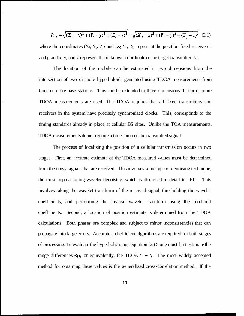
R,,j = , / ( X i - ~ ) 2 + ( Y , - y ) 2 + ( Z i - z ) 2 - , / ( X j - ~ ) 2 + ( Y j - y ) 2 + ( Z j - z ) 2 (2.1)

where the coordinates (Xi, Yi, Z,) and (Xj,Yj, Z,) represent the position-fixed receivers i

and j, and x, y, and z represent the unknown coordinate of the target transmitter [9].

The location of the mobile can be estimated in two dimensions from the

intersection of two or more hyperboloids generated using TDOA measurements from

three or more base stations. This can be extended to three dimensions if four or more

TDOA measurements are used. The TDOA requires that all fixed transmitters and

receivers in the system have precisely synchronized clocks. This, corresponds to the

timing standards already in place at cellular BS sites. Unlike the TOA measurements,

TDOA measurements do not require a timestamp of the transmitted signal.

The process of localizing the position of a cellular transmission occurs in two

stages. First, an accurate estimate of the TDOA measured values must be determined

from the noisy signals that are received. This involves some type of denoising technique,

the most popular being wavelet denoising, which is discussed in detail in [lo]. This

involves taking the wavelet transform of the received signal, thresholding the wavelet

coefficients, and performing the inverse wavelet transform using the modified

coefficients. Second, a location of position estimate is determined from the TDOA

calculations. Both phases are complex and subject to minor inconsistencies that can

propagate into large errors. Accurate and efficient algorithms are required for both stages

of processing. To evaluate the hyperbolic range equation (2. l), one must first estimate the

range differences Rij, or equivalently, the TDOA ti - tj. The most widely accepted

method for obtaining these values is the generalized cross-correlation method. If the

10

transmitted signal is s(t), then the signal that arrives at one receiver, x(t), will be delayed

and corrupted by noise and is given by

where di is the delay time from the mobile to receiver one, ni(t) is noise, and a is the gain.

Similarly, the signal that arrives at another receiver, y(t), is given by

where dj is the delay time from the mobile to receiver two, nj(t) is the noise, and p is the

gain. The cross-correlation function between the two received signals is derived by

integrating the lag product of the two signals for a sufficiently long time period, T. This

function is given by

' 0

This approach requires that the receiving base stations share a precise time reference

and reference signals, but does not impose requirements on the signal transmitted by the

mobile. Note, that we can improve the S N R of the TDOA estimation by increasing the

integration interval, T. The maximum likelihood estimate of the TDOA is obtained from

the computed cross-correlation function. This estimate corresponds to the value of z that

maximizes the cross-correlation function, Eq. (3.3 ).

11

In. METHODS TO IMPROVE TDOA ESTIMATION

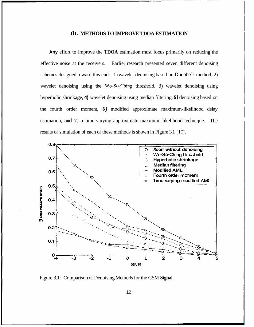
Any effort to improve the TDOA estimation must focus primarily on reducing the

effective noise at the receivers. Earlier research presented seven different denoising

schemes designed toward this end: 1) wavelet denoising based on Donoho’s method, 2)

wavelet denoising using the Wo-So-Ching threshold, 3) wavelet denoising using

hyperbolic shrinkage, 4) wavelet denoising using median filtering, 5 ) denoising based on

the fourth order moment, 6 ) modified approximate maximum-likelihood delay

estimation, and 7) a time-varying approximate maximum-likelihood technique. The

results of simulation of each of these methods is shown in Figure 3.1 [lo].

0 Hyperbolic shrinkage .:,::: Median filtering - Modified AML

-4 -3 -2 -1 0 1 2 3 4 5 SNR

Figure 3.1: Comparison of Denoising Methods for the GSM Signal

12

It was shown that method 1 failed at low SNR’s. Experimental results from [ 101

showed that method 2, while an improvement over method 1, looses its advantage with

increasing carrier frequency. Additional improvements are made using methods 3 and 4,

but as can be seen in Figure 3.1, the best results (lowest mean-square error) are obtained

using methods 5 through 7. We will take a closer look at method 5 and 6.

A. FOTJRTH-ORDER MOMENT WAVELET DENOISING

Inevitably, any transmitted signal will acquire some type of additive noise before

reaching the receiver. A Gaussian signal being completely characterized by its second

order statistics and the odd order moments being equal to zero for a symmetric

probability density function, the separation of the signal and the noise requires at least the

use of the fourth-order moments [ 1 11.

To define the fourth-order moment, we first model the received signal as:

z(n) = x(n) + Z(n) (3.1)

where x(n)is a complex zero-mean, non-Gaussian, fourth order stationary signal and

Z(n) is the noise, which is a complex zero mean-Gaussian signal independent of x(n) .

The fourth-order moment is then [ 1 11:

M4, ( j - i , k - i,l - i) = W z , , z j , Zk*, Zl*) (3.2)

It was shown that the fourth order moment of a detail function which contains the

4 4 signal should be greater than 3od, , where od, is the noise power at subband di [ 101.

By using this property, the wavelet coefficients that represent noise can be

eliminated while those having a signal dependency are retained. After modifying the

13

detail functions, the denoised signal is obtained by performing an inverse wavelet

transform using the modified coefficients.

B. MODIFIED APPROXIMATE MAXIMUM LIKELIHOOD DELAY

ESTIMATION

Critical to the task of source localization is the time delay estimation between

signals received at two spatially separated sensors in the presence of noise. If we let s(n)

represent the source signal, nl(n) and n2(n) represent the additive noises at the respective

sensors, and D is the difference in arrival times at the two receivers, then the receiver

outputs, rl(n) and r2(n), are given by

rdn) = a1 s(n) + ndn),

r2(n) = a 2 s(n - D) + n2(n),

n = O,l, ..., T-1

0 c al, a:! c 1

(3.3)

(3.4)

where T is the number of samples collected at each channel.

In the modified approximate maximum likelihood (MAML) delay estimation,

after wavelet decomposition and prior to cross-correlation, both the channel outputs are

optimally weighted at different frequency bands (i.e., scales). This weighting is done to

reduce the noise influence. The scaled subband components are combined using inverse

wavelet transform to construct the MAML prefiltered signal. The orthogonal wavelet

transform is attractive because in addition to being computationally efficient, it is less

sensitive to performance degradation in the estimation of D [12]. The final MAML delay

estimate is calculated from the location of the peak of the cross-correlation function of

the two denoised signals.

14

IV. SIGNAL SIMULATION AND TEST RESULTS

A. SIGNAL GENERATION

All test signals used in this project were generated using the Hewlett-Packard

Advanced Design System (HP-ADS). This provided an excellent method of obtaining

signals that are essentially the same as would be encountered in an actual cellular

communication receiver.

1. Advanced Design System

The HP-ADS program is an invaluable tool for the engineers representing many

different design aspects such as communications, digital signal processing, electronic

circuits, mechanical circuits, and many others. The communications package allows the

user to custom design any type of communications system, run simulations of the design,

and extract data collected from the simulation. Figure 4.1 shows the system used for the

signal simulation. A more detailed view of each of the major components of this system

can be found in Appendix [B].

2. GSM Signal Generation

One parameter that must be specified for the GSM signal generation is the sample

time. The specifications of the GSM signal were given in Chapter II. The HP-ADS

program specifies a symbol period of 3.7037 microseconds. The filter bandwidth is 1.2

MHz. This allows us to sample at a minimum frequency of 2.4 MHz without violating

the Nyquist criterion. For test purposes, we use three different sampling frequencies. As

15

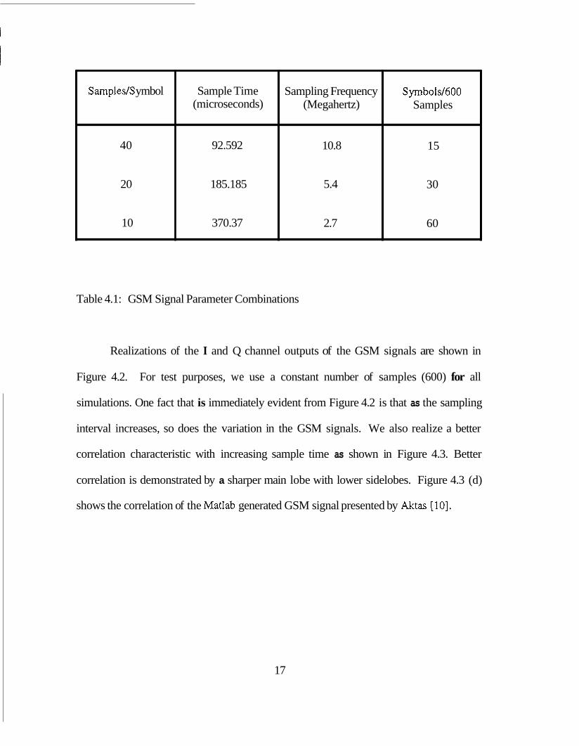
shown in Table 4.1, these are: 10.8 MHz, which corresponds to a sample time of 92.592

microseconds; 5.4 MHz, which corresponds to a sample time of 185.185 microseconds;

and 2.7 MHz, which corresponds to a sample time of 370.370 microseconds.

Design Name: GSM-SYS Purpose, To illustrate a basic GSM 0.3 GMSK system.Outputsindudeinputandwtputdata symbols. For a more detailed simulation, please open MODEM.

t - I 82

Figure 4.1 : Hp-ADS GSM Communications System

16

Samples/S ymbol

40

20

10

Sample Time (microseconds)

92.592

185.185

370.37

Sampling Frequency (Megahertz)

10.8

5.4

2.7

Symbols/600 Samples

15

30

60

Table 4.1: GSM Signal Parameter Combinations

Realizations of the I and Q channel outputs of the GSM signals are shown in

Figure 4.2. For test purposes, we use a constant number of samples (600) for all

simulations. One fact that is immediately evident from Figure 4.2 is that as the sampling

interval increases, so does the variation in the GSM signals. We also realize a better

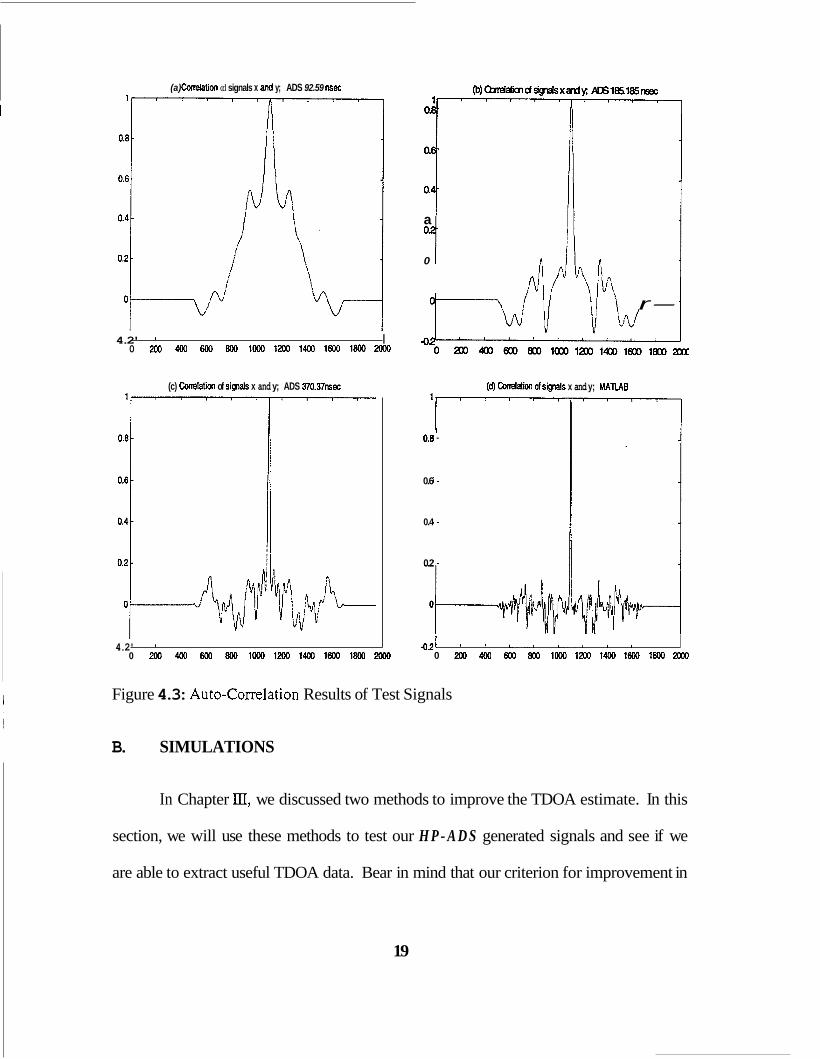
correlation characteristic with increasing sample time as shown in Figure 4.3. Better

correlation is demonstrated by a sharper main lobe with lower sidelobes. Figure 4.3 (d)

shows the correlation of the Matlab generated GSM signal presented by Aktas [lo].

17

(b) I channel; Ts = 92.592 ns (a) Qchamel, Ts = 92592 N

I 4 7

2 .

j 0

-2 ~

-4-

-6' I 0 100 200 3 0 0 4 0 0 500 600

(d) I Chanml; TS = 185.185 lls I

I 0 100 200 3 0 0 4 0 0 500 600

(9 I channel; Ts = 370.370 ns - 1 I

(c) Qm; Ts= 185.185 w 3 1

(e) Qdwrd; Ts =310.3?U w jl

0 100 200 3 0 0 4 0 0 500 600 9

Figure 4.2: HP-ADS Produced GSM Signals

'0 1 0 0 2 0 0 3 0 0 4 0 0 5 0 0 6 0 0

18

4.2' I 0 200 400 600 800 lo00 1200 1400 1600 1800 m

(a) cwrelation cd signals x and y; ADS 92.59 nsec

a

0 i r-

(c) Conelation of sigals x and y; ADS 370.37ns.x

4.2' I

0 200 400 600 800 lo00 1200 1400 1600 1800 m

(4 caratation d si@s x and y; MATIAB

I---- 0.8 -

0.6 -

0.4 -

0.2 -

Figure 4.3: Auto-Correlation Results of Test Signals

421 " " " " 0 m 400 600 800 loo0 1200 1400 1600 1800 m

B. SIMULATIONS

In Chapter III, we discussed two methods to improve the TDOA estimate. In this

section, we will use these methods to test our H P - A D S generated signals and see if we

are able to extract useful TDOA data. Bear in mind that our criterion for improvement in

19

TDOA estimation is a lower mean-squared error. Each method was tried using four

different realizations for each of the three sampling times, for a total of twelve different

realizations per method used. However, we will only present one set from each sample

time here, as each set follows a similar trend. The remainder of the plots can be found in

Appendix [C]. To simplify explanation, we shall label the data sets as follows:

a) HP-ADS generated signal with a sample interval of 92.59 nsec.

b) HP-ADS generated signal with a sample interval of 185.185 nsec.

c) HP-ADS generated signal with a sample interval of 370.370 nsec.

d) Matlab generated signal.

We will use the Matlab generated signal as our benchmark for comparison. For each

method we will plot the mean-squared error against SNR’s in the range of -6 dB to 20

dB. For clarity in the following discussion, we define the terms average error and

percentage improvement. Average error is calculated by adding all non-zero error values

for a particular realization, and dividing that sum by the total number of the non-zero

elements in that realization. Percentage improvement, as shown in the equation below, is

calculated by subtracting the improved value from the original value and dividing the

difference by the original value then multiplying by 100:

original value - improved value original value

x 100% = percent improvement

20

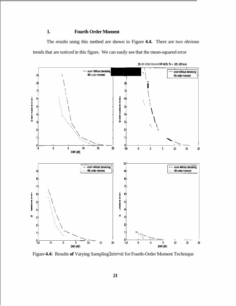
1. Fourth Order Moment

The results using this method are shown in Figure 4.4. There are two obvious

trends that are noticed in this figure. We can easily see that the mean-squared error

9- - xcov Without denoising

\, I- 4th order moment

8-

7- \ \ \

\ a -

7 -

6 -

5-

4 -

3 -

2 -

(b) 4th Order Moment HP-ADS; Ts = 185.185 nsec

\

I \ 1 I

9- - xconWithoutdenoising

i I

* i \ \

*\. \ \

10

9 -

8 -

7 -

f 6 -

-

I ---. 0 -10 -5 0 5 10 15 20 l t 1 I 1 ,I-

8-

7-

! 6 - 1 D ::

3-

2 -

1 -

1 % :I 3 -

2 -

1 -

1 . * , ' . 5- I ',\ ' 01

-10 -5 0 5 10 15 20 -10 -5 0 5 10 15 20 SNR (W SNR (W

01

Figure 4.4: Results of Varying Sampling Interval for Fourth-Order Moment Technique

21

improves (decreases) as the sampling interval increases. This observation is presented

numerically in Table 4.2. From this table, we can clearly see a decrease in error values as

we move from left to right across each row.

In the Matlab plot (Figure 4.4 (d)), or our benchmark plot, notice that the mean-

squared error is zero at 6 dB and higher SNR for the Fourth-Order Moment denoised

curve. Also notice that, as expected, the denoised curve is lower than the non-denoised

Mean Squared Error

caSe (a) case (b) caSe (c) (a S

N SampleTime = Sample Time = Sample Time = MatlabGenerated 92.59 nsec 185.185 nsec 370.370 nsec

R No Fourth- NO Fourth- NO Fourth- NO Fourth- Denoising Order Denoising Order Denoising Order Denoising Order

Denoising Denoising Denoising Denoising

-3

0

3

6

9

12

15

18

20

38.35

16.72

9.03

2.89

1.1 1

0.63

0.17

0.03

0

26.30

9.60

3.82

2.38

0.86

0.24

0.05

0.01

0

11.04

5.15

2.1 1

1.02

0.65

0.240

0.060

0

0

5.80 3.65 1.96 0.63 0.25

2.66 1.34 0.70 0.3 1 0.08

1.15 0.88 0.35 0.1 1 0.02

0.67 0.49 0.10 0 0

0.27 0.19 0.01 0 0

0.05 0.02 0 0 0

0 0 0 0 0

0 0 0 0 0

0 0 0 0 0

rable 4.2: Mean-Squared Error Values at Varying SNR for the Fourth Order Moment

22

curve at all points. This shows that the denoising is effective in producing an improved

TDOA estimate.

Using the HP-ADS data with a sampling interval of 92.59 nsec, case(a), the mean-

square error at -3 dB S N R is 26.3 when fourth-order denoising is employed. This is a

3 1.4% improvement from the non-denoised curve. The average percentage improvement

over all SNR’s between -3 and 20 is 45.6%.

Using HP-ADS data with a sampling interval of 185.185 nsec, we notice an

average 52.2% increase with fourth-order moment denoising. The mean-squared error is

5.68 at -3 dB, which is a 78.4% improvement over the -3 dB value of case (a).

Using H P- A D S data with a sampling interval of 370.37 nsec, case (c), we obtain

even better results. The mean-squared error at -3 dB is now 1.96, which is a 65.5%

improvement over case (b). The average improvement realized by using fourth-order

moment denoising instead of the non-denoised method in this case is 69.0%. We now

see a definite trend that as our sampling interval increases, denoising increasingly

improves the mean squared error values.

In the benchmark case (d), there is a maximum mean-squared error of 0.25 at -3

dB using fourth-order denoising. The average percentage improvement of fourth-order

moment denoising over non-denoising is 72.5%. We also notice that the mean-squared

error is zero for all SNR above 6 dB.

The improvements we have discussed in this section can be related to the

correlation function plots presented in Section 4.A. There, we saw that the correlation

function plot improved with increasing sample time. Here, we state that improved

23

correlation of the signal components reduces the probability of error in the TDOA

calculations. Thus, we achieve lower mean square error values with increasing degree of

correlation of signal components.

2.

The results using this method are shown in Figure 4.5. We notice a similar trend

as in the fourth order moment method. We end up with lower mean squared error values

Modified Approximate Maximum Likelihood (MAML)

(a) MAML WADS; Ts = 92.59 llsec @) MAML HP-ADS TS = 185.185 ~ L S B C

\ , 10 I 8 10

4th order moment - XCOR Whan dmslng

9 - \ \

8 - \ 8 -

7 - i 7 -

\ - 3 - \

i \

\

-.. \ \ \

\ 2 - / 3 -

2 -

1.

1 - '. r- - \ 1 - \.

0 I - -- 0 -10 -5 0 5 10 15 20 -1 0 -5 0 5 10 15

SNR (a) SNR (dB)

(cj MAMLHP-ADS: TS = 370.37 nsec

SNR (W)

(d) MAML; Matlab 10

.......... Modified AML 9 -

a -

? -

3 -

2 -

1 - \

0- -10 -5 0 5 10 . 15

\ '. ...... t 2 .... :- ........................ 1 ............ : ...................................

SNR (dB) 3

Figure 4.5: Results of Varying Sample Times for MAML Technique

24

as the sampling interval increases. We also notice that these mean squared error values

are lower than those obtained in the fourth order moment method, as evidenced in Table

4.3.

In case (a), there is an average improvement in mean squared error of 89.6% by

employing MAML denoising. Recall, from Section 4.B. 1, the fourth order moment - S

N

R

-3

0

3

6

9

12

15

18

20

-

Mean Squared Error

case (a) SampleTime = 92.59 nsec No I MAML

4.18 38.35

16.72

9.03

2.89

1.11

0.63

0.17

0.03

0

case (c) case (d)

11.04 1.37 3.65 0.47 0.63 0.09

2.27 5.15 0.60 1.34 0.25 0.31 0.01

1.05 2.1 1 0.27 0.88 0.08 0.1 1 0

0.43 1.02 0.13 0.49 0.02 0 0

0.22 0.65 0.02 0.19 0 0 0

0.10 0.240 0 0.02 0 0 0

0 0.060 0 0 0 0 0

0 0 0 0 0 0 0

0 0 0 0 0 0 0

Table 4.2: Mean-Squared Error Values at Varying SNR for MAML Method

25

denoising method produced only an average 45.6% improvement for case (a). Thus, we

have proved that the MAML denoising method is, in fact, superior to the fourth order

moment. In cases (b) and (c), there is an average improvement of 89.5% and 88.8%

respectively. Thus, we have shown that using the Hp-ADS program, we can simulate

GSM signals and obtain the necessary TDOA estimation. Application of the fourth order

moment and modified Approximate Maximum Likelihood methods reduce the error in

the TDOA estimation, allowing improved localization. In the current implementation the

MAML method outperforms the fourth order moment method. Matlab code can be found

in appendix D.

26

IV. SUMMARY AND CONCLUSIONS

A. SUMMARY

The objectives of this work are to simulate GSM signals and to evaluate the mean

squared-error for TDOA estimation. The Hewlett-Packard Advanced Design System is a

very powerful communications development tool and proved invaluable toward our

objective of GSM signal generation. We were able to manipulate this system to provide

signals with desired characteristics which would later be used in the Matlab environment

to determine the effectiveness of two different denoising methods. The denoising

methods were presented in earlier research. These are the fourth-order moment and

modified approximate maximum-likelihood methods. We used three signal sets

generated by the H P- A D S program to test the performance of each of these methods.

The results of these tests agreed with the earlier research. It showed that the current

implementation of the MAML method is the best choice.

B. FUTUREWORK

Follow on work should extend the algorithms to time-varying scenarios. An

extension to determine the performance in a fading environment should also be

undertaken. In addition, the situation when a weak signal is present in one channel and a

stronger signal in the other channel, should be examined. One should also revisit the

denoising techniques to develop improved versions.

27

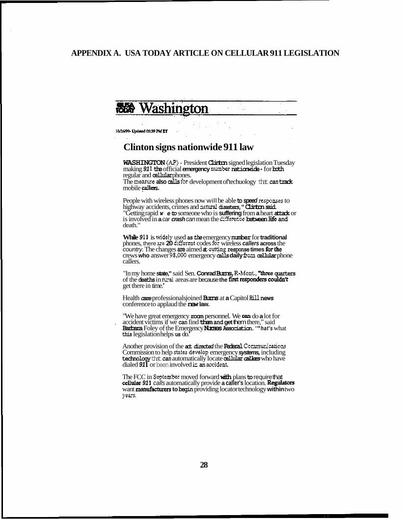
APPENDIX A. USA TODAY ARTICLE ON CELLULAR 911 LEGISLATION

Clinton signs nationwide 911 law WASHINGTON (Ap) - President Clinton signed legislation Tuesday making 91 1 the official emergency nmbex nationwide - for both regular and cellular phones. The measure also calls fm development of'techuology that can track mobile y e n .

People with wireless phones now will be able to speed responses to highway accidents, crimes and natural disasters," Clinton said. "Getting rapid w e to someone who is suffering from a heart attack or is involved in a car crash can mean the difference between M e and death."

While 9 1 1 is widely used as the emergency number for traditional phones, there am 20 merent codes lFor wireless callers across the country. The changes are aimed at cutting response times forthe crews who answer 98,000 emergency calls daily fhm cellular phone callers.

"In my home state," said Sen. Conrad Burns, R-Monk, "three quarters of the deaths in rinstl areas are because the 5st respondem couldn't get there in time.''

Health care professionals joined Burns at a Capitol Hill news conference to applaud the new law.

"We have great emergency room personnel. We can do a lot for accident victims if we can find them and get them there," said Barbara Foley of the Emergency Nurses Association. '"hat's what this legislation helps us do.''

,

Another provision of the act directed the Federal Communications Commission to help states deveIop emergency systems, including technology that can automatically locate cellular callers who have dialed 91 1 or been involved in an accident

The FCC in Septemkr moved forward with plans to require that cellular 91 1 calls automatically provide a caller's location. Regukdors want man- to begin providing locator technology within two Y-*

28

Privacy advocates have raised concerns about potential abuse of the tcchnology. which would take advantage of the Global Positioning System developed by the military.

The law signed Tuesday called on regulators to establish “appropriate privacy protection for Cali location information,” including systems that provide automaiic notification when a vehicle is involved in an accident.

It said that calls could only be tracked in nonemergency situations if the subscriber had provided written approval. ”The customer must “rant such authority expressly in advance of such use, disclosure or kcss,’’ according 10 Senate documents detailing provisions of the !e$slatioii.

An estimated 700 small and rural counties have no coordinated emergency service to call - eveu with traditional phones. The bill ivould encourage private 91 1 providers to move into those areas by eranting the same liability protections to wireless operations that now b e offered to wireline emergency service systems.

Scparately, the FCC took action earlier this year to increase the number of cellular calls to 91 1 that are successllly completed. The commission required that new arialog cellular phones - not existing phones - be made with sohvare that routes 91 1 calls to another carrier when a customer‘s own service cannot complete the call.

Calls sometimes arcn‘t completed because a caller is in an area where his or her carrier does not have ar. antenna, because networks are overloaded or because buildings or geography block signals.

Digital phones, of which 18.8 million now are in use? were not covered by the new FCC rules adopted in May because such phones arc nore complex than their analog counterparts and there is no easy fix for the problem.

-, , . ”, .. ..” . . . . . . - - __

LACE cor Premier vendors

Fmnt page News Sports 1yloney, Life, Weg@r,JAdietp@ 6 copynqhr 1999 USA TODAY, a divlsion of Gannet Co. Inc.

29

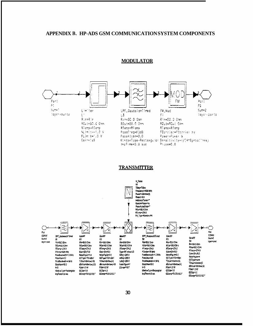
APPENDIX HP-ADS GSM COMMUNICATION SYSTEM COMPONENTS

MODULATOR

30

B.

II -.-1 -,---~ II :l <QH•F-' ---*-~ --~~.:[ 1. ·.~~ !... .. _..., ..... 1----~ ..... a.~l ~ ll-_..., .... 1----~ .... a.~i 11f .. /.'. n nl ~ . . ,-- ... ... . . I'-/ I ... ....i 'V'' I ' I ,, I J , r i ,-..,. . j , ., • · , V L/1

?~ ~: . ~ ' i "'-/ ' .l .r ~.:-.. ~#.. ..l.·, .o~ ·'· •.·

I!L~ _! 1 l · -.-- i' II ?2

em~ i'::!R T e~~,p L i rr:! :::- ~ . C V

LPF_Gc~ss!onTimed

L3 R i r=.SO. 0 Ohm

RTemp-::::Ricm;:> Passf>eq=f3dS P~;;:$Ai ~en=3.C

w;~dowType;q~c:cng~!c~

irr:pT!me=O.O sec

TRANSMITTER

' i* \ t !

II ... '' •.I l' \j i =;==

t

N.Tones N1 TStepoTstep ~1=8lOMHz "-~=llt>m!OW(S)

Phml.O.O ht!ilior.a!Tones:'" Ranallti!P!Iise•No Pllz~l~w

ROJI•SD.O Ol!m RT emp=-274.6 PN.T1;.e•Rar.C9mPN

FM_Mod

RCu t=~:~i t Cnm ~Temo=RTc~p

Carr i~r=~"Cr;rr ·r.r ~z

ensi t; \J i ty~1/~:!.·S:~b~: lme) r:;;se=C. D

r= • · I·

o~·-..... •!'~~:~~~:~-·~·">:! ~ · r "-' !! 1:/~:;1 IV"'~r!J ~ ,._¥ __ ( -· _., CONN: Num=l i>'f't=::t>:l:l

BPF_SllttffliOti~Tillllltl

81 Rir,:SO.o or.m ROt:•so.o 01rm RTell'p=·Zi'.C FCefl!e~)l)f;iHz

i'o>S63ndv.idlil=l2 1.!!'~ ~en=3D eope .. ,:iwicft,~~ u~~ ~111=SC.O N=3 WlllltwTypo•ROdangular lm;lirne=C.Osec

Giii:RF G1 RII\=SO.COhm ROur-50~ OIHn RTemp::-27~.0

Gain=22+j'O.O NeiseFPQur~•U

GCi!P'!"l'Ol+dScl TOI®t=<i~OW(·I3)

d!IC1~4mtow{-23)

I'Sat=l.OW GCSat•1.0 GComp='O.O 0.0 W

G:liollF G2 Riti=SD.OOhtn ROIJ:=SD,O Cllm RTem~r-2i4,0 ~22+j'll.O

N~F' ... IF3.5 GCT)pe•TO~d8c1

TOIOOI"!!lm~Nj-31

dBci0~1·10)

PSat:tCW GCsafoU GComFQ.OO.OW

lberRF 1.!1 Rll\=50.00ilm ROui•SO.O Ol!m RTt1111J"-274.0 Type=RFII!inlls!.O i<IRej=-<00.0 lmR~ ... 200.0 loRej:·200.0 liois!F'IQtllt"i tCcmp:'-1.5"

Bl'F.Il!JI!el\l'o:t\Timed 92 Rln=SO.OOhm ~out=SO.O Ollm RTemp=-274.0 FC~et=70 MHz P~.h=1.2MH%

PassAllen=3.0 St~'F4!1Hz

~c N•3 WilldowType:R~

1mPT1111e=O.Osee

GaL'iRr G3 llin=50.00hm ROur-50,001lm RTtmp:-274.0 G31r!=ZJ+i'O.O Noiref",gao;::l.S GCTr.e•TOI'1!Sc1 TOIOOI=dllm'~'S)

deelout--dll!nto'o(·S) Ps.tl!t:1.0W GC~1.0

GCo.'llp='n.OO.OO.O'

Goi!!RF G4 Ri,.SO.OOhm Rout•SO.O Ollm RTemp=-274.0 Go""25>;'0.0 ~F'IIj..e-4

GCType."~'.cflt

TO!llut=d"..mt0\'(5} !ISciD!l~-5) PSar-I,OW GCSit"1.0 GComp--"0.0 0.0 C.O •

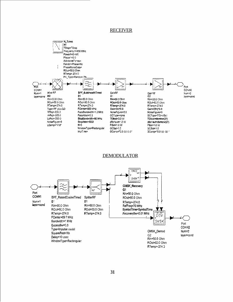
RECEIVER

TStep=TStep L I Frequencyl-830 MHz

Pwerl=5 mW Phasel.0 0 AddibonlToies: RandonPhase=No : PnaseNoiseData: ROui=50OOhm RTewp-2i4 0 PN-Type=Random,PN_-

1-

EPF-ButkwodhTmed GainRF CONNi ~~~~l MixerRF layet=wrid M2

Rln=50.0 Ohm ROut=53.0 Ohm RTemp=-274.0 T w R F plus LO RfRej=-200.0 lmRej=-200.0 LoRej=-200 0 NoiseFigure-8 LCOClp=-7.5"

E l Rln-50.0 Ohm ROuP5O.O Ohm RTemp274.0 FCenter=gOO MHz PassBa&dth=l.i MHr PassAttend.0 StopBandwidth=80 MHz StopAtten-50.0 N=3 WindowType=Reaangular ImpTime=

G1 Rln=SO.O Ohm ROutS50.0 Ohm

Gain=S+rO.O NoiseFigure=3.5 GCType=none TOlOut.r3.0 W dEclwt=l.O W PSat=l.O w GCSat=l.O GComp"0.0 0.0 0.0"

RT~p=-274.0

DEMODULATOR

Port CONN2

GainRF Num=2 layemmd 6 2

Rln=SO.O Ohm ROut=SO.O Ohm RTemps274.0 Gain=25+j'O. 0 NoiseFigure-6 GCType=TOl+dBcl TOlout==taw(37) dEc1 wt=dbmow(Z7) PSaP1.0 W GCSat=l .O GComp='O.O 0.0 0.0 "

CO"l BPF-RaisedCosineTimed SplitterRF

IaFFWnd RIn=50.0 Ohm Rln=50.0 Ohm ROut=50.0 Ohm ROut=50.0 Ohm RTemp=-274.0 RTemp274.0 FCented9.7 MHz Bandwidth=l MHz ExcessBw=O.O Type=lmpulse model SquareRoot=No Delay=lO usec WindowType=Rectanguiar

Num=l 81 s1 j i i

Rln=50.0 Ohm ROvl=50.0 Ohm RTmp=-274.0 ? RefFreq='IO MHz i 1 SymbOlTimeSymbolTime I RecoveryBw=O.Ol MHz 1

Port CONN2

GMSK-Demcd Num=2 G2 layer=cond Rln=50.0 Ohm ROut=50.0 Ohm RTemp=-274.0

31

APPENDIX C. MATLAB SIMULATIONS FOR EACH DATA SET

FOURTH ORDER MOMENT & MAML FOR SAMPLE TIME = 92.592 nsec

Results for DATA 92 set1

4th order moment Modmed AML

'i \

t \

i

I -5 0 5 10 15 SNR in (dB)

Results for DATA 92 set3

- xcorr wiulwt denoising

60

y....

P n F rn l e , 31 0 -4 n

70 -

60-

50 -

40-

E M 30-

20-

10 -

n-

Results for DATA 92 set2

4th order moment ........... M & i AML i

\

.. .... ... --...

" -10 -5 0 5 10 15 20

SNR in (dB)

Results for DATA 92 set4 80

I - XCOR without denoisina mt \

-9 1 I" I" -. -1V

SNR in (a)

32

SNR in (a)

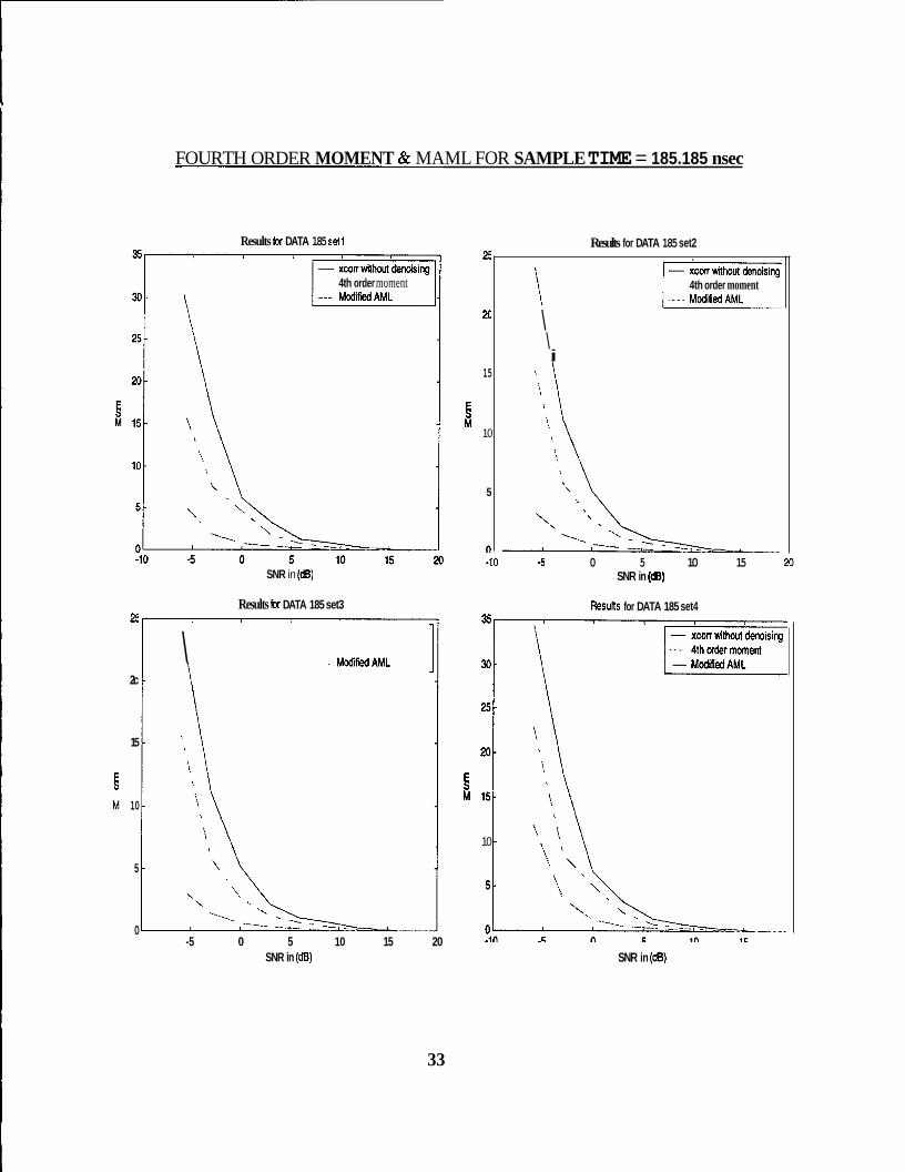
FOURTH ORDER MOMENT & MAML FOR SAMPLE TIME = 185.185 nsec

Results for DATA 185 sell

4th order moment

2!

2c

15

E M 10

5

0

SNR in (dB)

Results kx DATA 185 set3

\ i - - M~difiedAML

, \

',\ \ : \

-5 0 5 10 15 20 SNR in (dB)

25

x

15

E M

10

5

0

Results for DATA 185 set2

4th order moment

\ \ i

-10 -5 0 5 10 15 20 SNR in (dB)

Results for DATA 185 set4

30 - MCdiiedAML

25-

20-

E M 15-

10 -

SNR in (dB)

33

FOURTH ORDER MOMENT & MAML FOR SAMPLE TIME = 370.37 nsec

Results for DATA 370 set1 Results for DATA 370 set2

- xcwrvithout demising - 4thordermoment

Modlied AML

i

SNR in (dB)

Results for DATA 370 set3

- xcw Hithoui denasing

SNR in (dB)

a i I - xconwittnut demising I

7t \ - 4thordermment Modfied AML

SNR in (dB)

Reslsts for DATA 370 set4 a

- 4thordermoment 7 -

6 -

5 -

!i4 M

3 -

-10 -5 0 5 10 15 20 SNR in (dB)

34

APPENDIX D. MATLAB CODES

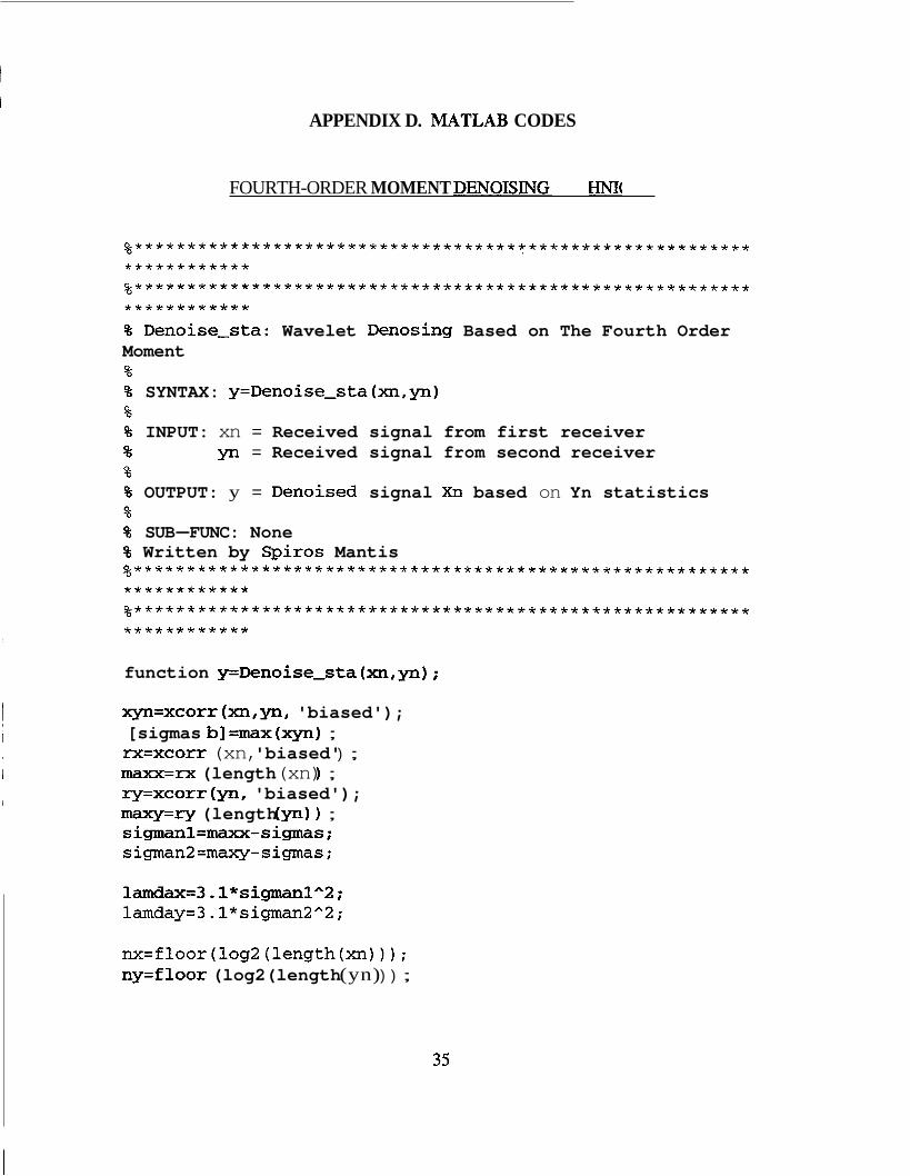
FOURTH-ORDER MOMENT DENOISING TECHNIOUE

. . . . . . . . . . . . . . . . . . . . . . . . . . . . . . . . . . . . . . . . . . . . . . . . . . . . . . . . . . .

. . . . . . . . . . . . . . . . . . . . . . . . . . . . . . . . . . . . . . . . . . . . . . . . . . . . . . . . . . .

% Denoise-sta: Wavelet Denosing Based on The Fourth Order Moment % % SYNTAX: y=Denoise-sta(xn,yn) % % INPUT: xn = Received signal from first receiver % yn = Received signal from second receiver % % OUTPUT: y = Denoised signal X n based on Yn statistics % % SUB-FUNC: None % Written by Spiros Mantis . . . . . . . . . . . . . . . . . . . . . . . . . . . . . . . . . . . . . . . . . . . . . . . . . . . . . . . . . . .

. . . . . . . . . . . . . . . . . . . . . . . . . . . . . . . . . . . . . . . . . . . . . . . . . . . . . . . . . . .

* * * * * * * * * * * *

* * * * * * * * * * * *

* ***********

* * * * * * * * * * * *

function y=Denoise-sta(xn,yn);

xyn=xcorr(xn,yn, 'biased'); [sigmas b]=max(xyn) ; rx=xcorr (xn, 'biased' ) ; maxx=rx (length (xn) ) ; ry=xcorr(yn, 'biased'); maxy=ry (length (yn) ) ; sigmanl=maxx-sigmas; sigman2=maxy-sigmas;

lamdax=3.1*sigmanlA2; lamday=3.l*sigman2"2;

nx=floor(log2(length(xn))); ny=f loor (log2 (length (yn) ) ) ;

35

[cx 1x3 =wavedec (xn, nx, ' db4 ) ; [ cy lyl =wavedec (yn, ny, ' db4 ) ;

dxc=[l; for i=l:nx

d=detcoef (cx, lx, i) ; dl=length (d) ; A=(l/dl)*sum(d."4);

if A-damdax

else

end

dc=zeros (1, dl ;

dc=d;

dxc= [dc dxcl ; end

a=appcoef(cx,lx, 'db4',nx); al=length (a) ; A=(l/al)*sum(a.^4);

if A< lamdax

else

end

ac=zeros (1, a1 1 ;

ac=a;

dxc=[ac dxc];

xd=waverec(dxc,lx,'db4');

y=xd;

36

. . . . . . . . . . . . . . . . . . . . . . . . . . . . . . . . . . . . . . . . . . . . . . . . . . . . . . . . . . .

. . . . . . . . . . . . . . . . . . . . . . . . . . . . . . . . . . . . . . . . . . . . . . . . . . . . . . . . . . . * * * * * * * * * * * *

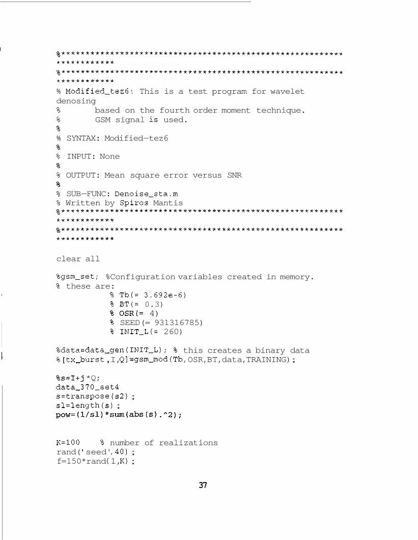
* * * * * * * * * * * * % Modified-tez6: This is a test program for wavelet denosing % based on the fourth order moment technique. % GSM signal is used. % % SYNTAX: Modified-tez6 % % INPUT: None % % OUTPUT: Mean square error versus SNR % % SUB-FUNC: Denoise-sta.m % Written by Spiros Mantis . . . . . . . . . . . . . . . . . . . . . . . . . . . . . . . . . . . . . . . . . . . . . . . . . . . . . . . . . . . * * * * * * * * * * * * . . . . . . . . . . . . . . . . . . . . . . . . . . . . . . . . . . . . . . . . . . . . . . . . . . . . . . . . . . . * * * * * * * * * * * *

clear all

%gsm-set; %Configuration variables created in memory. % these are:

% Tb(= 3.692e-6) % BT(= 0.3) % OSR(= 4) % SEED(= 931316785) % INIT-L(= 260)

%data=data-gen(IN1T-L); % this creates a binary data % [ tx-burst , I, Ql =gsm-mod (Tb, OSR, BT, data, TRAINING) ;

%s=I+j *Q; data-370-set4 s=transpose ( s 2 ) ; sl=length ( s ) ; pow=(l/sl)*sum(abs(s) . " 2 ) ;

K=100 % number of realizations rand( I seed' ,40) ; f =15 0 *rand ( 1, K) ;

37

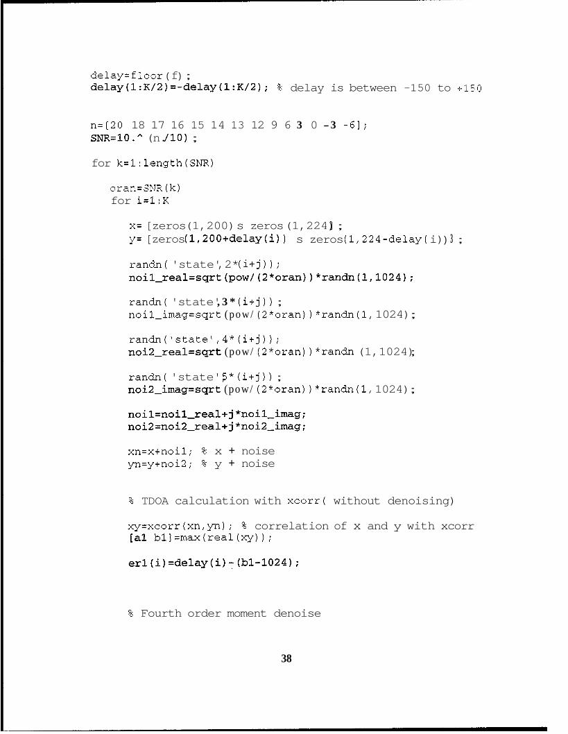
delay=f loor ( f ) ; delay(l:K/2)=-delay(l:K/2); % delay is between -150 to +150

n=[20 18 17 16 15 14 13 12 9 6 3 0 -3 -63; SNR=lO. (n. /lo) ;

for k=l:length(SNR)

oran=SNR (k) for i=l:K

x= [zeros (1,200) s zeros (1,224) 3 ; y= [zeros (1,2OO+delay(i) ) s zeros (1,224-delay( i) ) 3 ;

ran&( 'state' ,2* (i+j)); noil~real=sqrt(pow/(2*oran))*randn(l,lO24);

ran&( 'state' , 3 * (i+j) ) ; noil-imag=sqrt ( pow/ (2*oran) ) *randn(l, 1024) ;

randn('state1,4*(i+j)); noi2_real=sqrt (pow/ (2*oran) ) *randn (1,1024) ;

ran&( 'state', 5* (i+j) ) ; noi2_imag=sqrt (pow/ (2*oran) ) *randn(l, 1024) ;

noil=noil-real+j*noil-imag; noi2=noi2_real+j*noi2_imag;

xn=x+noil; % x + noise yn=y+noi2; % y + noise

% TDOA calculation with xcorr( without denoising)

xy=xcorr(xn,yn); % correlation of x and y with xcorr [a1 bl]=max(real(xy));

% Fourth order moment denoise

38

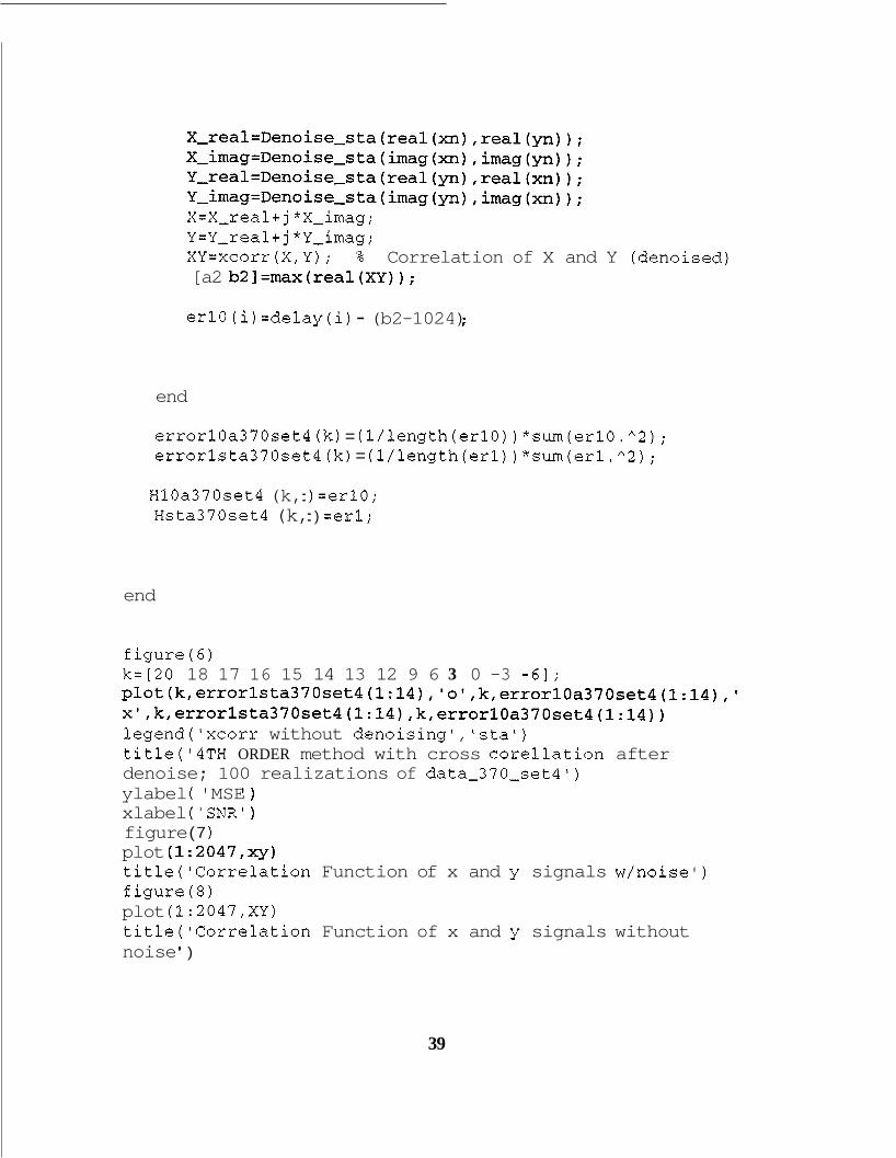
X-real=Denoise-sta(real(xn),real(yn)); X-imag=Denoise-sta(imag(xn),imag(yn)); Y-real=Denoise-sta(real(yn),real(xn)); Y-imag=Denoise-sta(imag(yn),imag(xn)); X=X-real+j*X-imag; Y=Y-real+j*Y-imag; XY=xcorr(X,Y); % Correlation of X and Y (denoised) [a2 b2]=max(real(XY));

erlO (i) =delay(i) - (b2-1024) ;

end

errorlOa370set4 (k) = (l/length(erlO) ) *sum(erlO. "2) ; errorlsta370set4 (k) = (l/length(erl) ) *sum(erl. "2) ;

HlOa370set4 (k, : ) =erlO; Hsta370set4 (k, : ) =er1;

end

figure(6)

plot(k,errorlsta370set4(l:l4),",k,errorlOa37Oset4(l:l4),i x',k,errorlsta370set4(l:l4),k,errorlOa37Oset4(l:l4)) legend('xcorr without denoising','sta') title('4TH ORDER method with cross corellation after denoise; 100 realizations of data-370-set4') ylabel ( 'MSE I ) xlabel ( ' SNR' ) figure (7 ) plot (1:2047,=) title('Corre1ation Function of x and y signals w/noise') figure(8) plot (1 :2047 ,XY) title('Corre1ation Function of x and y signals without noise I )

k=[20 18 17 16 15 14 13 12 9 6 3 0 -3 -61;

39

save errorlOa370set4; save errorlsta370set4;

save Hsta370set4; save HlOa370set4;

40

MODIFIED APPROXIMATE MAXIMUM LIKELIHOOD DENOISING

TECrnIOUE

. . . . . . . . . . . . . . . . . . . . . . . . . . . . . . . . . . . . . . . . . . . . . . . . . . . . . . . . . . .

. . . . . . . . . . . . . . . . . . . . . . . . . . . . . . . . . . . . . . . . . . . . . . . . . . . . . . . . . . .

% Denoise: Approximate maximum-likelihood delay estimation % via orthogonal wavelet transform. In this function, % we assumed that noise is Gaussian noise and it has a % flat freq response. We modify each detail function % by multipliying modified AML coefficient based on % the signal and noise powers. % % SYNTAX: y=amll(xn,yn) % % INPUT: xn = Received signal from first receiver % yn = Received signal from second receiver % % % OUTPUT: % y = Denoised signal % % SUB-FUNC: None % Written by Spiros Mantis . . . . . . . . . . . . . . . . . . . . . . . . . . . . . . . . . . . . . . . . . . . . . . . . . . . . . . . . . . .

. . . . . . . . . . . . . . . . . . . . . . . . . . . . . . . . . . . . . . . . . . . . . . . . . . . . . . . . . . .

* * * * * * * * * * * *

* * * * * * * * * * * *

* * * * * * * * * * * *

* * * * * * * * * * * *

function y=denoise(xn,yn);

xyn=xcorr(xn,yn,'biased'); [sigmas b] =max (xyn) ; rx=xcorr(xn, 'biased'); maxx=rx (length (xn) ) ; ry=xcorr(yn, 'biased'); maxy=ry (length (yn) 1 ; sigmanl=maxx-sigmas; sigman2=maxy-sigmas;

41

nx=f loor (log2 (length (xn) ) ) ; ny=floor(log2(length(yn)));

[cx lx]=wavedec(xn,nx, ' d b 4 ' ) ; [cy lyl=wavedec(yn,ny, 'db4');

dxc=[]; f o r i=l:nx

d=detcoef (cx, lx, i) ; dl=length (d) ; sigmad=(l/dl)*sum(d."2); sigmasd=sigmad-sigmanl; sigmaa(i) = (2" (nx-1) ) *sigmasd; if sigmasd<=O

else wd=O;

wd=sigmasd/(sigmanl*sigman2+sigmasd*(sigmanl+sigman2)); end dc=wd* d ; dxc=[dc dxcl;

end

a=appcoef (cx,lx, ' d b 4 ' ,nx) ; al=length (a) ; aux=sum (sigmaa) ; sigmasa= ( (2%~) ) *sigmas-aux; if sigmasa<=O

else

end ac=wa*a; dxc=[ac dxcl ;

wa=O ;

wa=sigmasa/(sigmanl*sigman2+sigmasa*(sigmanl+si~an2));

xd=waverec (dxc , lx, ' db4 1 ; y=xd;

42

. . . . . . . . . . . . . . . . . . . . . . . . . . . . . . . . . . . . . . . . . . . . . . . . . . . . . . . . . . .

. . . . . . . . . . . . . . . . . . . . . . . . . . . . . . . . . . . . . . . . . . . . . . . . . . . . . . . . . . .

% % Modified-tez5: This is a test program for modified AML technique. In this % program, we used GSM signal. % % SYNTAX: Modified-tez5 % % INPUT: None % % OUTPUT: Mean square error versus SNR % % SUB-FUN: Den0ise.m % Written by Spiros Mantis . . . . . . . . . . . . . . . . . . . . . . . . . . . . . . . . . . . . . . . . . . . . . . . . . . . . . . . . . . .

. . . . . . . . . . . . . . . . . . . . . . . . . . . . . . . . . . . . . . . . . . . . . . . . . . . . . . . . . . . .

* * * * * * * * * * * *

* * * * * * * * * * * *

* * * * * * * * * * * *

* * * * * * * * * * * *

clear all

gsm-set; %these are:

% Configuration variables created in memory.

% Tb(= 3.692e-6) 96 BT(= 0.3) % OSR(= 4) % SEED(= 931316785) % INIT-L(= 260)

data=data-gen(1NIT-L); % this creates a binary data [ tx-burs t , I, 41 =gsm-mod (Tb, OSR, BT, data, TRAINING) ;

s=I+ j *Q; sl=length(s) ; pow=(l/sl)*sum(abs(s) . "2 ) ;

K=100 % number of realizations rand( 'seed',40); f =15 0 *rand ( 1, K) ;

43

delay=f loor ( f ) ; delay(l:K/2)=-delay(l:K/2); % delay is between -150 to +150

n=[20 18 17 16 15 14 13 12 9 6 3 0 -3 -61; SNR=lO. (n. /lo) ;

for k=l:length(SNR)

oran=SNR (k) for i=l:K

x=[zeros(1,200) s zeros(1,224)]; y= [zeros (1,20O+delay(i) s zeros (lr224-delay( i) ) 3 ;

ran&( 'state' ,2* (i+j)); noil-real=sqrt (pow/ (2*oran) ) *randn(l, 1024) ;

randn(lstate1,3*(i+j)); noil-imag=sqrt (pow/ (2*oran) ) *randn(l, 1024) ;

randn ( state' ,4* (i+ j ) ) ; noi2_real=sqrt (pow/ (2*oran) ) *randn(l, 1024) ;

randn ( I state' ,5 * (i+j) ) ; noi2_imag=sqrt (pow/ (2*oran) ) *randn(l, 1024) ;

noil=noil-real+j*noil_imag; noi2=noi2_real+j*noi2_irnag;

xn=x+noil; % x + noise yn=y+noi2; % y + noise

% TDOA calculation with xcorr( without denoising)

xy=xcorr(xn,yn); % correlation of x and y with xcorr

[ a1 bl] =max (real (xy) ) ; %(with the presence of noise)

erl (i) =delay(i) - (bl-1024) ;

x_real=denoise(real(xn),real(yn)); % Denoising of the %received signals

44

y-real=denoise (real (yn) ,real (xn) ) ; x-imag=denoise (imag (xn) , imag (yn) ) ; y-imag=denoise (imag (yn) , imag (xn) ) ;

XY=xcorr(X,Y); % Correlation of X and Y (denoised) [a2 b2] =max(real (XY) ) ;

er8 ( i 1 =delay (i) - (b2-1024 ) ;

end

error8a(k)=(l/length(er8))*sm(er8.^2); errorla (k) = (l/length (erl) ) *sm(erl . "2) ; H8a(k, :)=er8; Hla(k, :)=erl;

end

figure ( 6 )

plot(k,errorla(l:14), 'o1,k,error8a(1:14), 'x',k,errorla(l:14 ) , k, error8a (1: 14) ) legend('xcorr without denoising','aml') title('Denoise AML method with cross corellation after denoise; 100 realizations') ylabel ( 'MSE ' ) xlabel ( ' SNR' ) figure (7) plot (1:2047 ,q) title('Corre1ation Function of x and y signals w/noise') figure ( 8 ) plot (1: 2047 ,XY) title('Corre1ation Function of x and y signals without noise ' )

k=[20 18 17 16 15 14 13 12 9 6 3 0 -3 -61;

save error8a; save errorla;

save Hla; save H8a;

45

LIST OF REFERENCES

1.

2.

3.

4.

5.

6.

7.

8.

9.

10.

11 .

Drane, C., Macnaughtan, M., and Scott, C., “Positioning GSM Telephones,” IEEE Communications Magazine, pp 46-59, April 1998

Mehrotra, A., GSM System Engineering, Norwood, MA, Artech House Publishers, 1997.

Rappaport, T. S., Wireless Communications: Principles & Practice, Upper Saddle River, NJ, Prentice Hall, 1996

Ibbetson, L. J., and Lopes, L. B., “Performance Comparison of Alternative Diversity Schemes Using a GSM Radio Link Simulation,” Mobile and Personal Communications, pp. 1 1 - 15, December 1993.

Joyce, R. M., Ibbetson, L. J., and Lopes, L. B., “Prediction of GSM Performance Using Measured Propagation Data,” University of Leeds, United Kingdom, 1996.

Hellebrandt, M., Mathar, R., and Scheibenbogen, M., “Estimating Position and Velocity of Mobiles in a Cellular Radio Network,” IEEE Transactions on Vehicular Technology, Vol. 46, No. 1, February 1997.

Aktas, U., and Hippenstiel, R., “Localization of GSM Signals Based on Fourth Order Wavelet Denoising,” 33d Asilomar Conference on Signals, Systems, and Computers, p 457-461, Oct 24-27, 1999, Pasific Grove, CA.

Hippenstiel, R., T.T. Ha, and Aktas, U., “Localization of Wireless Emitters Based on the Time Difference of Arrival (TDOA) and Wavelet Denoising,” NPSEC-99- 006, Naval Postgraduate School, Monterey, Ca, May 1999.

Rappaport, T. S., Reed, J. H., and Woemer, €3. D., “Position Location Using Wireless Communications on Highways of the Future,” IEEE Communications Magazine, pp 33-41, October 1996

M a s , U., Time Difference of Arrival (TDOA) Estimation Using Wavelet Based Denoising, Master’s Thesis, Naval Postgraduate School, Monterey, CA, March 1999.

Ferrari, A., and Alengrin, G., “Estimation of the Frequencies of a Complex Sinusiodal Noisy Signal Using Fourth Order Statistics,” Universite de Nice- Sophia Antipolis, Nice, France, 199 1.

46

12. Chan, Y. T., So, H. C., and Ching, P. C., "Approximate Maximum Likelihood Delay Estimation via Orthogonal Wavelet Transform," IEEE Transactions on Signal Processing, Vol. 47, No. 4, April 1999.

13. Hippenstiel, R., and Aktas, U., "Difference of Arrival Estimation Using Wavelets," 42nd Midwest Symposium on Circuits and Systems, p 1082-1085, Las Cruces, NM, August 8-1 1, 1999.

47

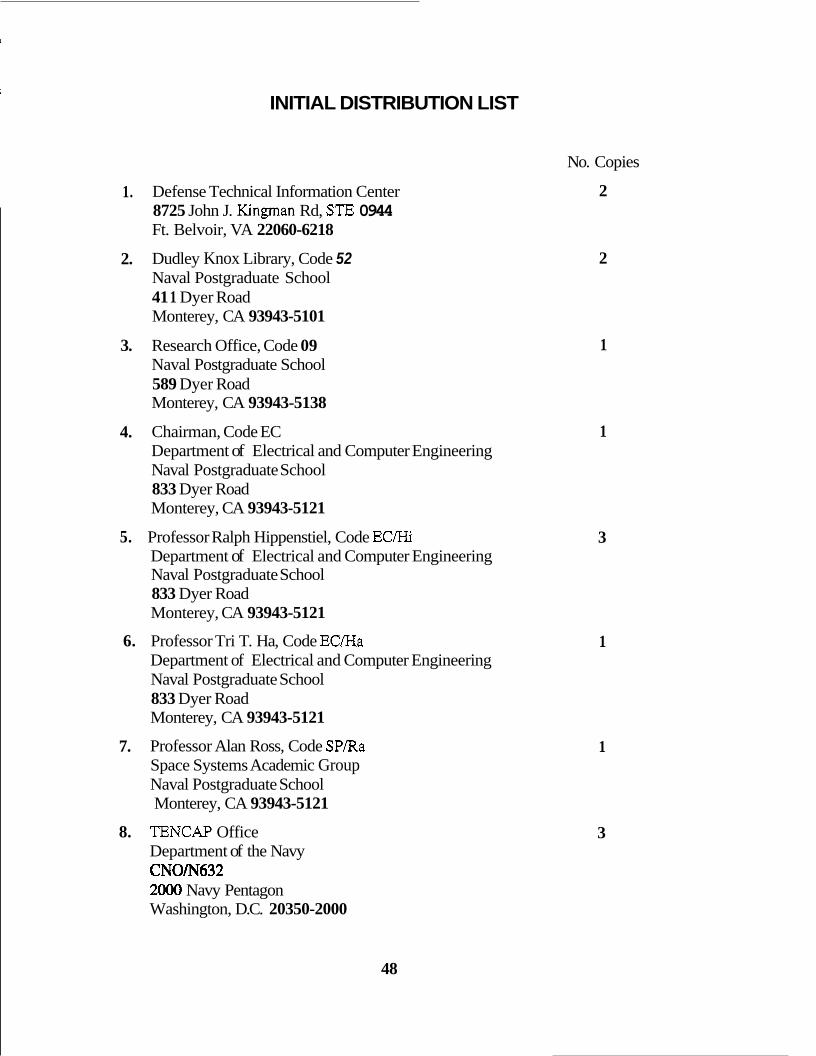
INITIAL DISTRIBUTION LIST

No. Copies

1.

2.

3.

4.

5.

6.

7.

8.

Defense Technical Information Center 8725 John J. Kingman Rd, STE 0944 Ft. Belvoir, VA 22060-6218

Dudley Knox Library, Code 52 Naval Postgraduate School 41 1 Dyer Road Monterey, CA 93943-5101

Research Office, Code 09 Naval Postgraduate School 589 Dyer Road Monterey, CA 93943-5138

Chairman, Code EC Department of Electrical and Computer Engineering Naval Postgraduate School 833 Dyer Road Monterey, CA 93943-5121

Professor Ralph Hippenstiel, Code EC/Hi Department of Electrical and Computer Engineering Naval Postgraduate School 833 Dyer Road Monterey, CA 93943-5121

Professor Tri T. Ha, Code EC/Ha Department of Electrical and Computer Engineering Naval Postgraduate School 833 Dyer Road Monterey, CA 93943-5121

Professor Alan Ross, Code SPRa Space Systems Academic Group Naval Postgraduate School Monterey, CA 93943-5121

TENCAP Office Department of the Navy CNO/N632 2000 Navy Pentagon Washington, D.C. 20350-2000

2

2

1

1

3

1

1

3

48