A COMPARATIVE FINANCIAL ANALYSIS OF FAST PYROLYSIS PLANTS IN

SOUTHWEST OREGON

By

Colin Brink Sorenson

B.S., Social Science, Kansas State University, Manhattan, KS 2001

Thesis

presented in partial fulfillment of the requirements for the degree of

Master of Arts in Economics

The University of Montana

Missoula, MT

May 2010

Approved by:

Perry Brown, Associate Provost for Graduate Education Graduate School

Dr. Helen Naughton, Chair Department of Economics

Dr. Tyron Venn

College of Forestry and Conservation

Dr. Douglas Dalenberg Department of Economics

Dr. Ranjan Shrestha

Department of Economics

ii

Sorenson, Colin B., M.A., May 2010 Economics

A comparative financial analysis of fast pyrolysis plants in southwest Oregon Chairperson: Dr. Helen Naughton

There are millions of acres of forestland in the Western United States that could benefit from fuel reduction treatments to improve forest health and reduce wildfire fuels. These treatments generate forest residues that are typically piled and burned. However, with increasing concerns about energy security, high oil prices, air quality from pile burning and climate change, there is great interest in examining ways to economically use these residues as a renewable energy source. Pyrolysis of forest biomass is one method that shows promise, though the financial feasibility of doing so has not been previously investigated. This study presents the expected financial performance of a mobile and a fixed pyrolysis plant in southwest Oregon, where stocks of forest biomass are high. The tradeoffs between using a smaller plant deployed in the forest and a larger centralized plant are then discussed.

Pyrolysis of forest residues involves using advanced technology to thermally degrade biomass in the absence of oxygen to produce bio-oil, biochar and syngas. The syngas is used entirely to provide thermal process energy for the pyrolysis system. Bio-oil can substitute for #2 fuel oil in some applications or be upgraded to produce higher value products. Biochar can be used as a substitute for coal or a valuable soil amendment that can sequester carbon and improve desirable soil properties such as water and nutrient holding capacity.

Information about costs, revenues and production rates for fast pyrolysis systems have been collected from existing pyrolysis firms and likely suppliers of goods and services to pyrolysis firms in Oregon. Financial performance is estimated using a discounted cash flow analysis to determine net present value (NPV) and internal rate of return (IRR) for each plant.

Benefits of an in-woods mobile plant include shorter biomass haul distances that contribute to a lower raw material input cost of $20 per bone dry ton (BDT), as opposed to $45 per BDT for the larger fixed-site plant. The ability to operate separate from the electrical grid and re-locate multiple times per year gives flexibility to the mobile plant. Advantages of the fixed plant include cost savings from economies of scale and lower bio-oil delivery costs. The baseline financial performance assessments for both plants are encouraging, with positive NPV and estimates of 7% and 21% IRR for the mobile and fixed plants, respectively. Sensitivity analyses have revealed that financial performance is particularly dependent on initial capital costs, labor and feedstock costs, and projected bio-oil and bio-char prices.

iii

Acknowledgements

I would first like to thank Helen Naughton for her tireless efforts to edit and

improve this thesis. Her guidance and support has been invaluable. My deepest gratitude

also goes out to Tyron Venn for inviting me to participate in this project and making

himself available every step of the way. I was continually impressed by his pleasant

nature, sharp mind, and relentless work ethic. It was a pleasure to work with everyone in

the economics department during my time there. I counted on Doug Dalenberg for his

sage advice and excellent teaching skills. Ranjan Shrestha provided assistance in the

early stages of my thesis work and important suggestions at the end. Stacia Graham’s

combination of wisdom and wit was always refreshing.

I also acknowledge the USDA Forest Service Research and Development

Program on Biomass, Bioenergy, and Bioproducts, which funded this project. It has been

an honor to work with the team here in Missoula including Greg Jones, Dan Loeffler,

Nate Anderson, Woody Chung, and Edward Butler, as well our project collaborators in

Alabama, Idaho, and Oregon. Special thanks also go out to the kind people that

contributed to this work by addressing my seemingly endless questions in our emails,

phone calls and meetings.

Finally, I thank my wife and our entire family for their love and support in all of

our endeavors.

iv

Table of contents

Page

Abstract ............................................................................................................... ii Acknowledgments........................................................................................................ iii Table of contents .......................................................................................................... iv List of tables .............................................................................................................. vi List of figures ............................................................................................................. vii List of equations ......................................................................................................... viii Chapter 1: Introduction ..................................................................................................1 1.1 Motivation for research ......................................................................................1 1.2 Case study ..........................................................................................................2 Chapter 2: Review of climate change implications and biomass conversion methods within the renewable energy framework .......................................8 2.1 Bioenergy and climate change implications ......................................................8 2.2 Renewable energy in the United States and Oregon ........................................11 2.3 Bioenergy conversion technologies .................................................................12 2.3.1 Thermochemical conversion of biomass ................................................13 2.3.2 Biochemical conversion of biomass .......................................................15 2.4 Pyrolysis technology ........................................................................................17 2.4.1 Slow pyrolysis .........................................................................................17 2.4.2 Fast pyrolysis ..........................................................................................18 2.5 Bio-oil characteristics ......................................................................................19 2.6 Biochar characteristics .....................................................................................20 2.7 North American fast pyrolysis system producers ............................................22 Chapter 3: Previous literature ......................................................................................24 3.1 Introduction ......................................................................................................24 3.2 Transport and harvest cost models ...................................................................24 3.3 Pyrolysis cost studies .......................................................................................26 Chapter 4: Data ............................................................................................................30 4.1 Introduction ......................................................................................................30 4.2 Production and plant assumptions ...................................................................31 4.3 Costs ..............................................................................................................33 4.3.1 Capital costs and financing .....................................................................34 4.3.2 Labor costs ..............................................................................................38 4.3.3 Delivered feedstock and loading costs ....................................................39 4.3.4 Process energy consumption and costs ...................................................41 4.3.5 Repair and maintenance costs .................................................................44 4.3.6 Product delivery costs .............................................................................44 4.3.6.1 Bio-oil delivery costs .....................................................................45

v

4.3.6.2 Biochar delivery costs ....................................................................47 4.3.6.3 Tar delivery costs ...........................................................................47 4.3.7 Insurance costs ........................................................................................48 4.3.8 Taxes and depreciation ...........................................................................49 4.3.9 Mobile plant initial mobilization and annual relocation costs ................50 4.4 Benefits ..............................................................................................................51 4.4.1 Bio-oil revenue........................................................................................52 4.4.2 Biochar revenue ......................................................................................53 4.4.3 Salvage revenue ......................................................................................54 Chapter 5: Financial analysis methods ........................................................................56 5.1 Introduction ......................................................................................................56 5.2 Discounted cash flow analysis and net present value ......................................56 5.3 Internal rate of return .......................................................................................60 5.4 Payback period .................................................................................................61 5.5 Sensitivity analysis...........................................................................................62 5.6 Breakeven analysis...........................................................................................63 Chapter 6: Financial performance of mobile and fixed-site pyrolysis plants ..............65 6.1 Introduction ......................................................................................................65 6.2 Mobile plant financial performance .................................................................65 6.3 Fixed plant financial performance ...................................................................67 6.4 Sensitivity analysis...........................................................................................68 6.4.1 Mobile plant sensitivity analyses ............................................................69 6.4.2 Fixed plant sensitivity analyses ..............................................................73 6.4.3 Mobile plant breakeven values ...............................................................77 6.4.4 Fixed plant breakeven values ..................................................................78 Chapter 7: Conclusion..................................................................................................80 References ..............................................................................................................84 Appendix A Additional sensitivity analyses ............................................................93 A.1 Mobile plant sensitivity analyses ....................................................................93 A.2 Fixed plant sensitivity analyses.......................................................................94 Appendix B Cost parameter tables ...........................................................................96 Appendix C Fixed plant wages and benefits ..........................................................101 Appendix D U.S. corporation income taxes ...........................................................103 Appendix E Recent No. 2 fuel oil prices ................................................................104

vi

List of tables

Table Page

2.1 Typical product yields from pyrolysis of wood ...............................................17 4.1 Production and plant assumptions ...................................................................32 4.2 Cost and revenue assumptions .........................................................................35 4.3 Dirksen & Sons bio-oil delivery estimate (cents per gallon) ...........................45 5.1 List of cost and benefit variables .....................................................................58 6.1 Mobile plant cash flow projections, NPV and IRR .........................................66 6.2 Fixed plant cash flow projections, NPV and IRR ............................................67 6.3 Mobile plant NPV under multiple pricing scenarios for bio-oil and biochar ..73 6.4 Fixed plant NPV under multiple pricing scenarios for bio-oil and biochar .....77 B.1 Mobile plant delivered feedstock costs ...........................................................96 B.2 Mobile plant feedstock loading costs (Caterpillar 262 Skid Steer) .................96 B.3 Mobile plant energy consumption and costs ...................................................97 B.4 Mobile plant bio-oil delivery costs..................................................................97 B.5 Mobile plant biochar delivery costs ................................................................97 B.6 Fixed plant initial capital investment ..............................................................98 B.7 Fixed plant investment and financing costs ....................................................98 B.8 Fixed plant labor costs.....................................................................................98 B.9 Fixed plant delivered feedstock costs..............................................................99 B.10 Fixed plant feedstock loading costs (Caterpillar 914G Wheel Loader) ........99 B.11 Fixed plant energy consumption and costs .................................................100 B.12 Fixed plant bio-oil delivery costs ................................................................100 B.13 Fixed plant biochar delivery costs ...............................................................100 D.1 Federal tax rate schedule for 2008 ................................................................103

vii

List of figures

Figure Page

1.1 Map of study region in southwest Oregon .........................................................4

1.2 Renewable Oil International, LLC fast pyrolysis process .................................6

2.1 Renewable energy consumption in the nation’s energy supply, 2008 .............11

2.2 Conversion options for biomass to energy ......................................................13

4.1 Market locations for bio-oil and biochar .........................................................46

6.1 Mobile plant NPV sensitivity to several important cost variables ...................70

6.2 Mobile plant NPV sensitivity to bio-oil and biochar prices ............................72

6.3 Fixed plant NPV sensitivity to several important cost variables .....................75

6.4 Fixed plant NPV sensitivity to bio-oil and biochar prices ...............................76

E.1 U.S. No. 2 distillate price by all sellers, Sep 2007-Aug 2009 .......................104

viii

List of equations

Equation Page

4.1 ..........................................................................................................................52

5.1 ..........................................................................................................................59

5.2 ..........................................................................................................................59

5.3 ..........................................................................................................................59

5.4 ..........................................................................................................................59

5.5 ..........................................................................................................................59

1

Chapter 1

Introduction

1.1 Motivation for research

Decades of fire suppression throughout the Western United States have created

large areas of densely-stocked forests that could benefit from mechanical thinning to

reduce wildfire fuels (Rummer et al. 2005). Rapidly increasing greenhouse gas (GHG)

emissions since the industrial revolution have led to climate-related environmental

problems, largely from the burning of fossil fuels (IPCC 2007). Due to erratic oil and gas

prices, energy security through increased domestic renewable energy production has

become a high priority (Perlack et al. 2005). There is a growing desire for dynamic

solutions to these problems which often require collaborative efforts from universities,

government agencies and private firms. In the forest products sector, pyrolysis of forest

biomass for the production of bio-oil and biochar may be part of the answer. However, in

order for a course of action to be adopted its financial feasibility must be examined.

Sustainable production of bioenergy through pyrolysis of forest biomass is a

means of substituting away from fossil energy and meeting land management objectives.

These objectives include decreasing wildfire fuels, reducing fire suppression costs and

improving soils while addressing climate change issues. A study by Perlack et al. (2005)

found that native forest productivity creates 370 million dry tons of available biomass in

the United States each year. Pre-commercial thinning and fuel reduction forestry

practices generate slash, or biomass, which is commonly either left to decay or handled

via open burning.

2

Public land managers are required to remove biomass to reduce wildfire fuels, but

methods of doing so can be cost-prohibitive due to the low value and high moisture

content of the biomass, especially as biomass haul distance increases (Loeffler 2004;

Silverstein et al. 2006). Therefore, there is considerable interest in finding biomass

removal and utilization methods that are financially viable. This is the primary

motivation for research on the potential for mobile in-woods pyrolysis and the tradeoffs

between mobile and fixed-site systems. Implementing a mobile pyrolysis system reduces

feedstock haul distance, the largest factor in determining total feedstock cost, by allowing

the system to be located near existing stocks of biomass. Higher feedstock costs at fixed-

site pyrolysis plants are offset by economies of scale in the production process that allow

more efficient use of inputs, especially labor. The net effect of these tradeoffs on

financial performance is quantified in this analysis.

This research may serve as a guide for land management agencies considering

various biomass utilization options, as well as prospective investors in the forest products

industry. The results and sensitivity analyses presented highlight the most important

factors that determine financial feasibility of fast pyrolysis operations using forest

biomass as feedstock. While this study is based on pyrolysis plants in southwest Oregon,

various parameter levels could be adjusted to apply the results to another region.

1.2 Case study

It has been stated that bio-oil can be economically produced in-woods and

transported out of forests to end users (Badger and Fransham 2006). This analysis

investigates that claim in the context of southwest Oregon using existing data, expert

3

opinions, and cost estimates from likely providers of goods and services to a pyrolysis

firm in the region. Additionally, a discounted cash flow analysis (DCFA) has been

conducted to highlight net present value (NPV) and internal rate of return (IRR) for two

hypothetical pyrolysis plants with an expected operating life of 10 years—a fixed-site

200 bone dry ton per day (BDTPD) plant located in Glide, Oregon and a mobile 50

BDTPD plant that is assumed to relocate twice per year on public lands throughout

southwest Oregon. Payback period was also determined for each plant.

I examine the financial feasibility of utilizing available biomass via pyrolysis and

compare the performance of a 50 BDTPD mobile pyrolysis plant with a 200 BDTPD

fixed-site plant. The two systems are compared in order to quantify the tradeoffs

between the economies of scale with the fixed plant and lower feedstock costs with the

mobile plant. Assumptions have been based on costs and geographic features of

southwest Oregon, where biomass is particularly abundant.

The southwest region of Oregon, centered at Roseburg, is the study area for this

project. As depicted in figure 1.1, the region has a high percentage of forest cover. The

area is mostly comprised of Douglas Fir and Mixed Conifer forests, much of which are

now prone to intense wildfire due to management practices that have altered historic fire

regimes (OFRI 2002). Mechanical thinning, timber harvest, and restoration treatments

generate substantial stocks of forest biomass each year, representing a large potential

supply of bioenergy feedstock in the region (Cloughesy 2009). However, due to the high

cost of transporting slash, this biomass is typically disposed of via open burning. In

addition to the financial costs of open burning, social costs arise from particulate matter

emissions that decrease air quality (ODEQ 2009). Therefore, alternate biomass

4

utilization options with controlled emissions systems are attracting considerable interest.

Pyrolysis is particularly intriguing because of the co-products it produces—bio-oil, which

can substitute for liquid fossil fuels in certain applications, and biochar, which can be

applied to the land to achieve desirable results such as carbon sequestration and increased

soil fertility (Lehmann et al. 2006).

Figure 1.1 Map of study region in southwest Oregon

Source: Anderson (2010)

For both systems in this study, I assumed in-woods chipping of the feedstock

being transported to the pyrolysis plant. A short feedstock haul distance was

incorporated with the mobile plant financial model, which generated relatively low

feedstock costs. Conversely, the fixed plant feedstock will need to be sourced from a

5

larger supply region and transported a longer distance. A two-phase feedstock haul was

built into the fixed plant financial model. The first phase is a short haul to a

concentration yard in smaller-capacity trucks that can navigate narrow forest roads. The

second phase brings the feedstock the remainder of the distance to the plant in larger-

capacity chip vans, primarily on paved roads. The two-phase haul produced significantly

higher feedstock costs compared to the mobile plant feedstock costs on a per ton basis.

The pyrolysis process being considered in this analysis involves “moving bed reactors,”

shown in figure 1.2. This technology is patented by Renewable Oil International, LLC

(ROI), the industry collaborator on the project (Badger 2009c). Production costs and

pyrolysis system parameters were provided by ROI for a 50 BDTPD mobile plant and a

200 BDTPD fixed-site plant. However, up to now the largest plants ROI has

manufactured include a 5 BDTPD mobile plant and a 15 BDTPD fixed-site (modular)

plant. Therefore, the system requirements for the plants in this study are based on

projections calculated by ROI rather than observations.

6

Figure 1.2 Renewable Oil International, LLC fast pyrolysis process

Source: Badger (2009c)

The following outlines the ROI pyrolysis process as described by Badger (2008).

For optimal results, feedstock must be chipped down to a particle size that is no more

than 1/8th inch thick in at least one dimension to get the proper heat transfer rate. After

the feedstock is fed into the system it is dried down to 10% moisture content (30% initial

feedstock moisture content was assumed in the analysis). Feedstock is subsequently fed

into the reactor, where it is heated to approximately 480o Celsius within 1 second. The

vapors are then rapidly condensed into bio-oil and the biochar is extracted. Non-

condensable gas, or syngas, is re-circulated within the system to provide process energy.

After the pyrolysis process is complete, products are shipped to end-users. I

assumed that bio-oil would be sold as a substitute for No. 2 fuel oil to wholesale buyers

in the Portland area, and biochar would be sold as a soil amendment to wholesale buyers

Char

Heat Carrier

Gas & Vapor

Biomass

Moving Bed Reactor

7

within a 2.5 hour haul of the pyrolysis plants. Chapter 4 provides more detail on the

financial costs and benefits for each plant.

The remainder of this thesis is organized as follows: Chapter 2 includes

background information on the climate change implications of bioenergy use, followed

by a closer examination of the pyrolysis process and the products it renders. Previous

literature on forest biomass utilization and pyrolysis cost studies is reviewed in chapter 3.

I then lay out the input data used for the financial model in chapter 4 and the financial

analysis methods in chapter 5. The financial performance results of the mobile and fixed-

site pyrolysis plants and sensitivity analyses are presented in chapter 6. Finally, the

conclusions of this research are presented in chapter 7.

8

Chapter 2

Review of climate change implications and biomass conversion methods within the renewable energy framework

2.1 Bioenergy and climate change implications

Global climate change is perhaps the most pressing environmental issue humanity

currently faces. Our climate is regulated by greenhouse gases (GHGs) that trap heat in

the atmosphere to maintain temperatures necessary to sustain life on the planet.

However, anthropogenic GHG emissions have increased significantly since the pre-

industrial era. The Intergovernmental Panel on Climate Change (IPCC) declared with

“very high confidence” that since 1750 the net effect of human activities has been one of

warming (IPCC 2007). The major anthropogenic GHGs in the atmosphere are carbon

dioxide (CO2), methane (CH4) and nitrous oxide (N20). CO2 is the most pervasive of the

anthropogenic emissions and therefore GHG emissions are typically calculated based on

their global warming potential (GWP)1 in terms of CO2 equivalents (CO2-e) (IPCC

2007).

Atmospheric CO2 levels are increasing due to anthropogenic emissions from the

burning of fossil fuels and to a lesser extent from land use change. According to the

IPCC (2007), anthropogenic CO2 emissions grew by 80% between 1970 and 2004. This

perturbation of the natural carbon cycle contributes to increased warming potential in the

1 Methane (CH4) has a GWP 21 times that of CO2, and Nitrous Oxide (N2O) has a GWP roughly 310 times CO2. However, CO2 is still the largest overall source of anthropogenic emissions after accounting for differences in GWP (IPCC 2007).

9

atmosphere and negative externalities such as rising sea level, ocean acidification, erratic

weather patterns, and increased incidence of catastrophic forest fires (IPCC 2007).

Increasing the share of renewable (non-fossil) energy to our national energy mix

could serve as one strategy to mitigate anthropogenic GHG emissions. By incorporating

solar panels and wind turbines, a greater portion of electricity demand is met by

renewable sources. Using biomass or biochar in power plants can offset a portion of the

coal that is burned for electricity generation. Renewable liquid fuels such as ethanol,

biodiesel, and bio-oil can substitute for fossil-derived fuels such as gasoline and diesel

fuel oil.

Without a binding policy that regulates GHG emissions and puts a price on

emitting carbon, market failure exists. The marginal social costs of activities that emit

CO2 are greater than the marginal social benefits at the current level of consumption.

This leads polluters to generate emissions in excess of the socially efficient amount.

Polluters would need to be required to internalize the negative externalities they create in

order to correct this market failure. Such policies would encourage the use of renewable

energy.

Consumption of fossil energy such as coal and petroleum emits CO2 from the

pool of sequestered carbon. Sequestered carbon remains in the earth and does not

increase atmospheric CO2 concentration unless it is mined and consumed to satisfy

energy demand. The net addition of CO2 to the atmosphere makes fossil fuel

consumption a “carbon positive” practice.

Conversely, consumption of renewable energy is often referred to as “carbon

neutral” and occasionally even “carbon negative.” This is because carbon from these

10

sources would be released to the atmosphere through the carbon cycle whether used for

energy or not. The biomass used for renewable energy is considered part of the pool of

carbon that is in flux within the carbon cycle, as opposed to sequestered carbon which is

stored outside of the carbon cycle. Biomass takes in CO2 through photosynthesis and

releases CO2 when it eventually decomposes. Converting biomass to renewable energy

avoids the atmospheric CO2 that would be emitted through decomposition—instead, CO2

is emitted when the bioenergy product is consumed at the end of its life cycle. When a

portion of the carbon in biomass is diverted from the carbon cycle via pyrolysis and

stored in biochar soil amendments, the practice can be considered “carbon negative,” as it

results in a net decrease in atmospheric CO2 (Lehmann 2007; Winsley 2007; Matthews

2008; Laird et al. 2009; Amonette 2009).

Biochar is unique because it can be used as an energy product or as a soil

amendment with the ability to store carbon for hundreds or even thousands of years

(Cheng et al. 2008). Both of these options can serve to mitigate anthropogenic CO2

emissions, though according to Gaunt and Lehmann (2008), amending soils with biochar

results in greater anthropogenic emissions reductions than using it as a fuel.

While biochar soil applications may be desirable from a socio-economic

perspective, the practice is not likely to be adopted on a large-scale unless there is an

accompanying private benefit greater than or equal to the benefit that could be realized

through using it as a fuel source. As mentioned by Laird et al. (2009), government

policies that give incentives to reduce GHG emissions would make pyrolysis more

competitive with existing energy production technologies.

11

2.2 Renewable energy in the United States and Oregon

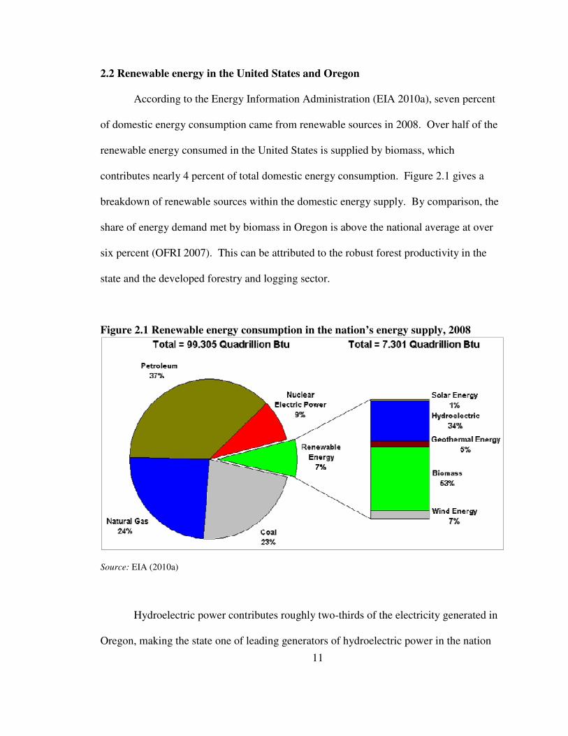
According to the Energy Information Administration (EIA 2010a), seven percent

of domestic energy consumption came from renewable sources in 2008. Over half of the

renewable energy consumed in the United States is supplied by biomass, which

contributes nearly 4 percent of total domestic energy consumption. Figure 2.1 gives a

breakdown of renewable sources within the domestic energy supply. By comparison, the

share of energy demand met by biomass in Oregon is above the national average at over

six percent (OFRI 2007). This can be attributed to the robust forest productivity in the

state and the developed forestry and logging sector.

Figure 2.1 Renewable energy consumption in the nation’s energy supply, 2008

Source: EIA (2010a)

Hydroelectric power contributes roughly two-thirds of the electricity generated in

Oregon, making the state one of leading generators of hydroelectric power in the nation

12

(EIA 2010b). This substantial hydroelectric potential contributes to the relatively low

electricity prices that the state enjoys (EIA 2010b). These low energy prices also reduce

the benefits of the mobile plant operating off-grid. The four largest electricity generation

facilities are hydroelectric plants located on the Columbia River. Considerable wind

energy potential also exists throughout much of Oregon, and the state accounts for 4

percent of total domestic wind energy generation (EIA 2010b).

2.3 Bioenergy conversion technologies

A thorough discussion of biomass sources and the options for producing energy

from biomass can be found in McKendry (2002a; 2002b). The two categories of

conversion technologies are thermochemical and biochemical (McKendry 2002b; Caputo

et al. 2005). Below are brief descriptions of biochemical and thermochemical conversion

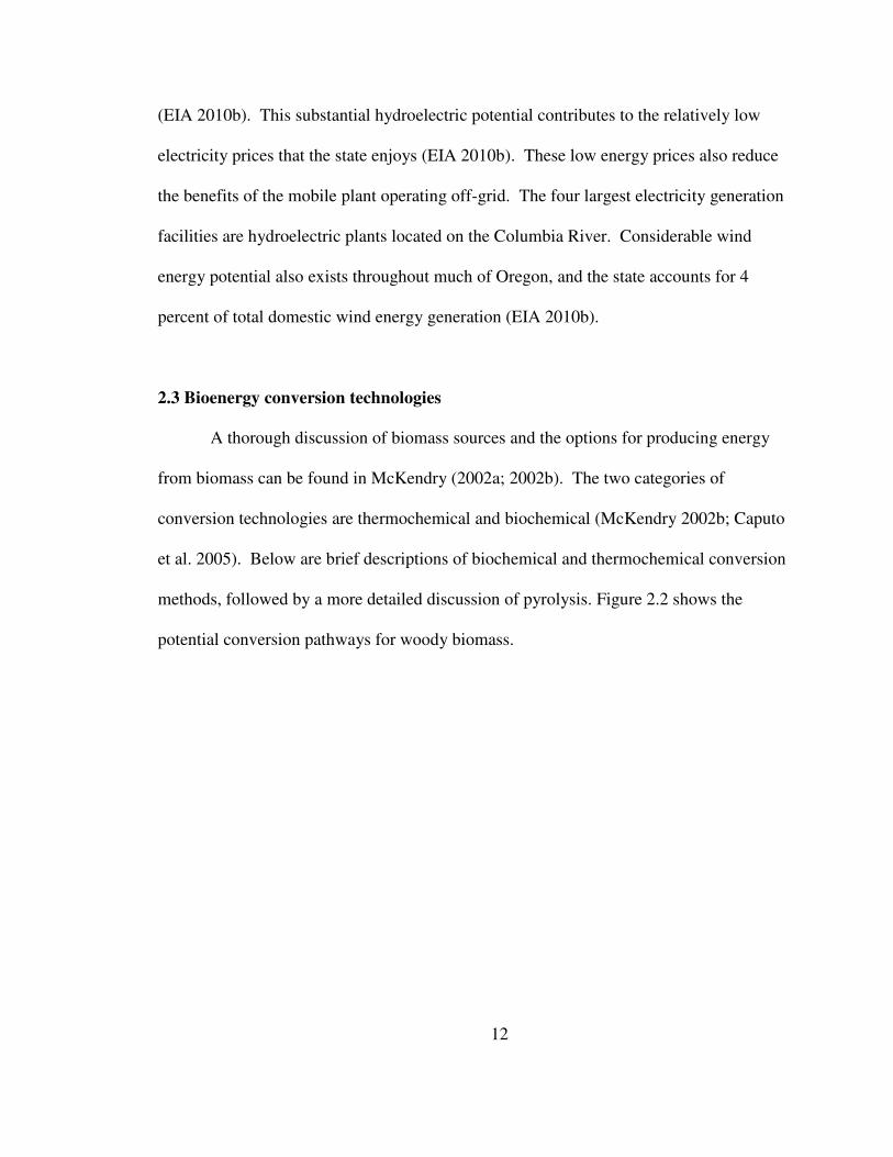
methods, followed by a more detailed discussion of pyrolysis. Figure 2.2 shows the

potential conversion pathways for woody biomass.

13

Figure 2.2 Conversion options for biomass to energy

Sources: McKendry 2002b; Caputo et al. 2005

2.3.1 Thermochemical conversion of biomass

Conversion of biomass by thermochemical means is accomplished through

combustion, gasification and pyrolysis (McKendry 2002b). The choice of conversion

technology depends on the desired end-use products and the characteristics and location

of the biomass feedstock. Pyrolysis is the first step in combustion and gasification as

well, though partial or total oxidation of the products occurs after pyrolysis in these

processes (Bridgewater 2007).

Combustion of biomass to generate energy involves burning in air to produce

heat, mechanical power or electricity. The scale of bioenergy production from

Thermochemical Biochemical

Combustion Gasification Pyrolysis FermentationAnaerobic

Digestion

Heat,

Steam,

Electricity

Producer gas,

Electricity

Bio-oil,

Biochar,

Syngas

Ethanol Biogas

Biomass

14

combustion can be very small (i.e. wood stove) to very large (i.e. commercial power

plant). Small-scale combustion to produce steam for electricity generation is

characterized by relatively low efficiency and potentially problematic emissions

(Bridgewater 2004). Due to high conversion efficiency of biomass at coal-fired power

plants, co-combustion of biomass with coal can be an attractive option for maximizing

biomass conversion efficiency (McKendry 2002b).

Biomass gasification occurs at temperatures of over 800o Celsius and typically

renders 85% gas, 10% char and 5% liquid (Bridgewater 2007). The gas portion of the

outputs, called producer gas, is most commonly used to generate electricity, though it can

also be processed through Fischer-Tropsch synthesis to produce renewable transportation

fuels (Kerns 2009). Unlike combustion, gasification is characterized by high efficiency

at all scales of operation (Bridgewater 2004). One of the downsides of gasification for

the production of electricity is that the system must be connected to the electrical grid in

order to deliver the final product. This limits the plausibility of an in-woods gasification

plant that utilizes forest residues, as in-woods operations could benefit from the ability to

operate at remote, off-grid sites.

Pyrolysis is the thermal decomposition of biomass occurring in an oxygen-free or

oxygen-restricted chamber to produce liquid, char and gas (Bridgewater 2004). Biomass

pyrolysis has been practiced for thousands of years in various capacities. In ancient

Egypt pyrolysis of biomass was used to produce tar for caulking boats and other

applications (Mohan et al. 2006). The existence of terra preta or “dark earths” of the

Amazon suggests that pyrolysis was used to create char for soil management hundreds

15

and thousands of years ago (Lehmann et al. 2006). More attention is given to pyrolysis

technology, products and producers in sections 2.4 through 2.7.

2.3.2 Biochemical conversion of biomass

Fermentation and anaerobic digestion are the biochemical methods of bioenergy

production. In the United States, fermentation is implemented on a large commercial

scale at corn ethanol plants. High moisture content biomass tends to be more suitable for

biochemical rather than thermochemical conversion (Matthews 2008).

The vast majority of ethanol produced in the United States is blended with

gasoline at concentrations of up to ten percent (E10). Ethanol is typically used as a

gasoline oxygenation additive to boost the octane level of the fuel and reduce carbon

monoxide emissions. Methyl tert-butyl ether (MTBE) has also been used for gasoline

oxygenation. However, its use has declined significantly in recent years due to

groundwater pollution concerns, and ethanol has been used in place of MTBE. Eighty-

five percent ethanol blends (E85) are also available in some regions of the country and

can be used in flex-fuel vehicles. The corn ethanol industry is the most mature biofuels

sector in the United States, with nine billion gallons produced in 2008 and 170

commercial plants in operation by January 2009 (RFA 2010).

Corn-based ethanol has been a contentious topic in agriculture and energy policy

in recent years. Several questions have been raised surrounding the associated ratio of

energy inputs to outputs (energy balance), effects on world food supply and prices

(Runge & Senauer 2007), and the direct and indirect land use changes resulting from

ethanol production (Searchinger et al. 2008). A full fuel-cycle analysis has shown that

16

energy balance and GHG emissions from ethanol plants vary widely, from slight

increases in overall GHG emissions if coal is used for process energy, to significant GHG

reductions if wood chips are used (Wang et al. 2007). It is important to evaluate the

merits and drawbacks of individual plants according to their specific characteristics,

especially regarding the sources and required amounts of process energy per unit of

output.

Cellulosic ethanol is lauded as a fuel with improved energy balance and fewer

concerns regarding food supply and land use change because it is produced from non-

food feedstocks (Lynd et al. 1991; Hill et al., 2006). However, the technology has not

been brought to market on a commercial scale due to high capital costs in comparison to

corn ethanol plants. The increased complexity associated with the conversion of

cellulose rather than starch has also contributed to the delay in bringing large-scale

cellulosic ethanol plants online (EIA 2007). Development of unique enzymes to simplify

the process and cut costs is a promising breakthrough that could bring cellulosic ethanol

to market in the near future (Bradley 2009).

Anaerobic digestion is the other biochemical pathway, involving the conversion

of organic wastes in the absence of oxygen to produce “biogas,” an energy-rich

combination of methane and CO2 (McKendry 2002b). The process is commonly

employed to treat wastewater and reduce GHG emissions.

Financial incentives from carbon credit projects have helped dairy and swine

producers install anaerobic digesters on their farms. Credits are generated by quantifying

the reduced methane emissions in terms of CO2-e as well as avoided fossil fuel

17

consumption (ClearSky 2010). Biogas can be used in turbines for electricity generation

or upgraded to a product similar to natural gas by removing the CO2 (McKendry 2002b).

2.4 Pyrolysis technology

While pyrolysis is certainly an ancient practice, only recently have scientists

understood the relationships between heat transfer rates and product yields and

distribution (Ringer et al. 2006). Table 2.1 shows the variation in product distribution

based on the mode and reactor conditions under which pyrolysis occurs. The product

distribution from Bridgewater et al. (2007) represents the high end of bio-oil yield in the

fast pyrolysis literature, and the product distribution from ROI (McGill 2009a) in the

table is at the lower end of reported bio-oil yields from fast pyrolysis.

Table 2.1 Typical product yields from pyrolysis of wood Yield, % feedstock wt Mode Conditions Liquid Char Gas Fasta Moderate temperature, ~480oC,

short residence time, ~1sec 57 27 15

Fastb Moderate temperature, ~500oC, short residence time, ~1sec

75 12 13

Slow (carbonization) Low temperature, ~ 400oC, very long solids residence time

30 35 35

Gasification High temperature, ~800oC, long vapor residence time

5 10 85

Source: Table adapted from Bridgewater (2007) Notes: a. Yields used in this study, based on ROI technology, assuming 1% tar byproduct (McGill 2009a)

b. Yields based on Bridgewater (2007) and Ringer et al. (2006)

2.4.1 Slow pyrolysis

Whether pyrolysis is “slow” or “fast” refers to the rate at which the biomass is

heated, though there is no precise definition of the heating rates or times that each refer to

18

(Mohan et al. 2006). Slow pyrolysis, also called carbonization, is a well established

technology that has historically been used to manufacture “charcoal.” Brown (2009)

defines charcoal as “char produced from pyrolysis of animal or vegetable matter in kilns

for use in cooking or heating.” Historical slow pyrolysis methods and the variety of

pyrolysis pits, mounds and kilns that have been used over time are discussed, as well as

suggestions for advancements in biochar system manufacturing (Brown 2009).

The slow pyrolysis product distribution of liquid, char and gas is roughly 30%, 35%

and 35% respectively (Ringer et al. 2006; Bridgewater 2007). When char is produced for

the purpose of applying it to soil for agronomic improvements or environmental

management, it is often called “biochar” (Lehmann and Joseph 2009).

2.4.2 Fast pyrolysis

Transitioning from slow to fast pyrolysis drastically shifts the distribution of

products in favor of bio-oil. Fast pyrolysis refers to rapid heating of a feedstock in the

absence of oxygen to produce char, vapors, and permanent or non-condensable gases

(Ringer et al. 2006). The vapors are quickly condensed to a dark brown liquid. Several

terms have been used to describe the liquid product, including pyrolysis oil, bio-crude,

liquid wood, wood oil, and bio-oil (Bridgewater 1999). Bio-oil is now the most common

term and will continue to be used for the remainder of this paper. The char and non-

condensable gases are hereafter referred to as biochar and syngas, respectively.

The product distribution of bio-oil, biochar and syngas can vary significantly

depending on the type of fast pyrolysis reactor used. Feedstock characteristics, including

particle size and tree species (for pyrolysis of woody biomass), can cause the product

19

output to vary as well, but to a lesser extent (Amonette 2009). Therefore, a range of

product distributions is more likely to be observed than a constant distribution. Based on

conversations with ROI (McGill 2009a), the product distributions chosen for the baseline

scenario in the methods section is 57 percent bio-oil, 27 percent biochar, 15 percent

syngas, and 1 percent tar2. This is assumed to be the most reasonable average

distribution of products over time.

2.5 Bio-oil characteristics

Bio-oil is the liquid product of fast pyrolysis. It is a free-flowing dark brown fuel

with a strong “smoky” smell and an energy density 6 to 7 times that of raw biomass

(Badger and Fransham 2006). Representing one of the newest sources of renewable

energy, bio-oil has the advantages of being readily storable and easily transportable

(Bridgewater 2002). With minimal modifications the fuel can substitute for liquid fossil

fuels in several stationary applications such as boilers, engines and turbines (Ensyn 2001;

Yaman 2004; Badger 2008; Bouchard 2009).

Bio-oil typically contains 15-30% water and oxygen accounts for roughly half of

its weight (Bridgewater 2002). The prevalence of water in the fuel is the primary reason

for several undesirable qualities in bio-oil, compared to petroleum-derived fuels. High

oxygen and water content in bio-oil reduces its energy density and increases its acidity

(Oasmaa and Czernik 1999). At ten pounds per gallon, the weight of bio-oil exceeds that

of number two fuel oil. Consequently, bio-oil contains approximately 60% of the energy

2 The presence of tar as a byproduct does not appear in the economics of fast pyrolysis literature, though in personal communication with ROI (McGill 2009) it was mentioned that a small amount, up to 1%, can be generated by their process.

20

content of No. 2 fuel oil on a volumetric basis, but only 40% of the energy content by

weight (Bridgewater 1999). Bio-oil does not mix well with hydrocarbon fuels and is not

as stable as fossil fuels due to phase separation over time (Bridgewater 2002).

2.6 Biochar characteristics

The carbon and energy dense solid obtained from the pyrolysis of biomass is

called biochar, especially when intended for use as a soil amendment (Brown 2009).

‘Char’ is the generic term used to refer to the material regardless of its end-use. The

product is called ‘charcoal’ when used as a fuel for heating or cooking, and sometimes

called ‘agrichar’ when applied to agricultural soils (Lehmann and Joseph 2009). The

term ‘biochar’ encompasses char used either for agriculture or to improve soils in other

contexts such as environmental remediation.

Biochar is a fine-grained, highly porous powder with several characteristics that

can foster desirable properties in soils (IBI 2010). The high porosity and large surface

area of biochar allow it to improve water and nutrient retention in soils. Biochar has also

shown the ability to increase cation exchange capacity (Laird et al. 2009), a common

measure for soil fertility. The effect of biochar on mycorrhizal associations and soil

microbes has been investigated, with evidence suggesting that biochar amendments could

increase microbial activity and thus improve fertilizer use efficiency and plant growth,

leading to economic and environmental benefits (Warnock et al. 2007; Laird et al. 2009).

When used as a soil amendment, biochar is part of a process that can

simultaneously produce renewable biofuels, sequester carbon, and improve degraded

soils. According to the IPCC (2000), over 80% of the organic carbon in terrestrial

21

ecosystems is in soil. Therefore, soils should be considered a good option for carbon

sequestration. According to Lal et al. (2004), promoting soil carbon sequestration

through recommended management practices has the potential to mitigate 5% to 15% of

global fossil fuel emissions.

The application of biochar to soils has been practiced for several millennia, as

evidenced by the highly fertile terra preta (“dark earth”) soils of the Amazon Basin

(Sombroek et al. 2003; Lehmann et al. 2006). It is believed that the soils were

purposefully amended with charred biomass by native inhabitants thousands of years ago.

Soils in the region that were amended with biochar currently store approximately 2.5

times the quantity of carbon compared to otherwise similar parent material soils in the

region that were not amended (Glaser et al. 2001). This suggests that biochar is very

stable in soils and a one-time amendment can deliver long term benefits to the soil.

Laird et al. (2009) provide a comparison of the carbon remaining in biomass over

time compared with biochar. For biochar, the amount of initial biomass carbon is

reduced by about 40% when pyrolysis occurs, and another 10% within a few months of

soil application. The remaining 50% is stable in soil for thousands of years. With

biomass residue, about half of the carbon degrades within 6 months, and only 1% of the

initial carbon remains after 4 years. This suggests that the concerns regarding soil carbon

and nutrient removal through extracting biomass residues for bioenergy production could

be addressed in part by applying biochar after removing residues.

22

2.7 North American fast pyrolysis system producers

While pyrolysis is a relatively new technology for large-scale energy

applications, it has been used to produce niche market chemicals for decades. Over 200

chemical compounds have been identified in bio-oil (Soltes and Elder 1981), and early

commercial pyrolysis applications almost exclusively involved the extraction of value

added chemicals.

Ensyn, headquartered in Ottawa, Ontario, was incorporated in 1984 to

commercialize its fast pyrolysis process. Over 30 bio-chemicals have been extracted

from Ensyn bio-oil, including flavoring products for the food industry and adhesive

resins for the construction industry (Ensyn 2010). Additionally, the company is engaged

in the production of bio-oil for stationary fuel applications and research and development

of renewable transportation fuels. Ensyn has two facilities in Wisconsin that process 40

and 45 metric tons of biomass per day (49.6 US tons), and a facility in Ontario with the

ability to process 100 metric tons per day (110.2 US tons) (Goodfellow 2008).

Dynamotive is a publicly traded pyrolysis firm based in Vancouver, British

Columbia, with additional offices in the United States and Argentina. Since 2001

Dynamotive has constructed fast pyrolysis facilities with increasing feedstock processing

capabilities (Dynamotive 2010). A 10 metric ton per day demonstration plant was

completed in British Columbia, and plants with the ability to process 130 and 200 metric

tons per day (143.3 and 220.4 US tons, respectively) were subsequently completed in

West Lorne and Guelph, Ontario, respectively. The West Lorne plant is co-located with

Erie Flooring and Wood Products and uses sawdust generated on site as the biomass

23

feedstock. A 2.5 megawatt Orenda turbine at the West Lorne plant has been fueled with

bio-oil to generate electricity for sale to the Ontario grid.

Advanced Biorefinery Inc. (ABRI) is based in Ottawa, Ontario and specializes in

multiple services involving energy and bio-products, including modular and mobile

pyrolysis units (ABRI 2010). ABRI has manufactured pyrolysis systems ranging from

0.5 BDTPD mobile units to 50 BDTPD modular units.

Renewable Oil International, LLC (ROI) is based in Alabama and specializes in

mobile and modular fast pyrolysis systems that can be pre-fabricated and shipped to their

destinations. ROI has manufactured 5 bone dry ton BDTPD mobile units and 15 BDTPD

modular units. ROI has provided many of the projected cost and production estimates

used to decipher the financial performance of the hypothetical mobile and fixed pyrolysis

plants analyzed in this study. Representatives from Dynamotive and Ensyn have also

provided helpful information during the course of this project.

The list of existing fast pyrolysis system producers in North America is fairly

short. In addition to the pilot plants and commercial-scale facilities that exist, research on

fast pyrolysis technology has taken place at multiple locations, including Iowa State

University, the University of Oklahoma, and the National Renewable Energy Laboratory

(NREL) in Golden, CO. In the next chapter, I discuss existing literature related to this

financial analysis of mobile and fixed pyrolysis plants in southwest Oregon.

24

Chapter 3

Previous literature

3.1 Introduction

This chapter discusses existing literature related to this project. I begin by

addressing transport and harvest cost models that consider the economic feasibility of

biomass utilization. Selected pyrolysis cost studies are then reviewed to set the context

of the current study.

3.2 Transport and harvest cost models

Several studies have looked at methods for handling small diameter wood

(biomass) from forestry operations and techniques to utilize the biomass as a feedstock

for bioenergy production. The economic feasibility of small wood harvesting and

utilization in southwest Idaho was examined by Han et al. (2004). Results indicated that

markets for forest biomass need to be located close to the harvest site in order for

biomass fuel harvesting to be feasible financially, and harvesting costs per unit volume

increase as size of tree declines. I find a similar trend with financial feasibility in my

analysis—the further the biomass needs to be hauled, the less likely the operation is to be

profitable. Han, et al. also cited limited accessibility to existing roads, hauling distance to

processing facilities, and low market prices for thinning materials challenges when trying

to implement biomass utilization practices in conjunction with a forest restoration and

thinning prescription.

25

A study by Silverstein et al. (2006) included biomass utilization modeling on the

Bitterroot National Forest in western Montana. The report compared fuel treatment

prescriptions on public lands and examined the economic tradeoffs of hauling the

material to different locations. Forest Inventory Analysis (FIA) data was used to identify

initial stand conditions and the Forest Vegetation Simulator (FVS) was used to simulate

forest growth and estimate volumes of removed material over time. The study was

developed to help public land managers and private investors make decisions regarding

the use of forest biomass as a renewable energy feedstock. Maximum net value per acre

figures were derived for each treatment prescription and incorporated with haul costs.

The results showed the high importance of biomass market location in relation to the

forest resources. The results showed that biomass utilization (compared with on-site pile

burning) was profitable in 97 percent of the areas with an average haul distance of 25

miles, but fell to 57 percent when the haul distance was increased to an average of 75

miles.

Biomass volumes and availability in Ravalli County, Montana, were determined

based on the “comprehensive treatment prescription” by Loeffler (2004). The

comprehensive prescription involves removal of all trees up to 7 inches in diameter at

breast height (DBH) and some larger trees, with a target residual basal area of 50 square

feet per acre. Available biomass volumes were estimated based on selected forest types

using Forest Inventory Analysis (FIA) data and remotely sensed GIS data, which

complemented each other in order to produce robust biomass estimates. Haul costs were

estimated using GIS by calculating the distance by road surface type (paved and

unpaved) from each polygon to the bioenergy production facility. The analysis showed

26

that a comprehensive treatment prescription would produce 12 to 14 green tons of

biomass per acre that could be delivered to a bioenergy facility in Ravalli County,

Montana. The Fuel Reduction Cost Simulator (FRCS) was used to estimate stump to

loaded truck harvest costs with the comprehensive prescription across all diameter

classes.

Although the harvest and transport cost models mentioned above provide insight

regarding estimated costs and common challenges, risks, and benefits inherent with forest

biomass utilization projects, they are different in nature than this study. The current

project involves using forest biomass that has already been generated through thinning

and restoration projects, so the decisions regarding treatment prescription are outside the

scope of this analysis. However, referring to the aforementioned studies in additional to

the financial analysis produced here could help stakeholders make informed decisions

while planning and implementing thinning and restoration prescriptions in combination

with biomass utilization projects, especially if utilization through pyrolysis is one of the

options being considered.

3.3 Pyrolysis cost studies

The University of New Hampshire considered using low-grade wood chips to

produce bio-oil and investigated the feasibility of using bio-oil as a replacement for No. 2

fuel oil for heat and electricity (Farag et al. 2002). After evaluating the technologies

designed by two Canadian pyrolysis firms, Ensyn and Dynamotive, they concluded that

the Dynamotive bubbling fluidized bed design was more suited to their objectives and

conducted the study based on that type of system. They analyzed production costs for

27

feedstock rates of 100, 200, and 400 wet wood (45% moisture content) metric tons per

day3, with a feedstock cost of $18 per wet metric ton.

The research found that it would cost roughly twice as much to use bio-oil instead

of No. 2 fuel oil in heat or electricity applications. This led the group to suggest further

research on using bio-oil for non-energy applications such as asphalt paving or “green

chemicals, ” though they did not carry out the suggested research. The Farag et al. study

also concluded that bio-oil would be cost-competitive with fossil fuels for producing heat

and electricity if the feedstock cost were to fall by 50% down to $9 per wet metric ton.

That would be equivalent to $18 per bone dry US ton with zero moisture content (BDT),

the units I use in my analysis.

My study on financial performance of pyrolysis plants in southwest Oregon

contributes to the literature by considering a mobile plant with lower feedstock costs, as

suggested by Badger and Fransham (2006). One major difference in the Farag et al.

study and the current study is that Farag et al. did not include revenue for biochar.

Instead, it was assumed to be used only for process energy in drying the feedstock. If the

study had assumed a char price similar to the $136 per ton chosen in my analysis, I

presume that bio-oil would have been cost-competitive with fossil fuels, even with if

feedstock costs were higher.

A study on the applications of bio-oil was conducted by Czernick and

Bridgewater (2004). They listed several conclusions on the challenges that must be

overcome in order for bio-oil to be a viable fuel in large-scale operations. Among the

3 One metric tonne is equivalent to 2204 pounds, or 1.102 US tons.

28

challenges cited was the ‘cost of bio-oil’ which was determined to be 10% to 100%

higher than the cost of fossil fuels. However, the study did not go into great detail on the

financial or energetic costs, making it difficult for that finding to be compared to the

findings in the current study on pyrolysis plants in southwest Oregon.

An overview of the technical and economic aspects of large-scale pyrolysis

production, as well as a more comprehensive list of previous pyrolysis studies, was

produced by Ringer et al. (2006) at the National Renewable Energy Laboratory (NREL).

The report provides information on the technical requirements for pyrolysis, several types

of pyrolysis reactor designs that can be implemented, and gives a detailed economic

analysis of a theoretical 550 metric ton per day plant using a fluidized bed reactor design.

In contrast, I consider a 50 BDTPD mobile plant and a 200 BDTPD fixed-site plant,

based on ROI fast pyrolysis technology. The pyrolysis reactors discussed in the Ringer et

al. study include fluidized beds (bubbling and circulating), ablative, vacuum, and

transported beds without a carrier gas. In contrast, I consider ROI pyrolysis systems that

use a mechanical auger reactor, also referred to as a moving bed (Badger 2009c).

An economic analysis of a 200 bone dry metric ton (BDMT) per day plant by

Dynamotive (2009) found a net production cost for bio-oil of $4.04 per GJ4. This is

equivalent to $0.74 per gallon of bio-oil on a volumetric basis was low enough to

generate positive returns in the analysis. Important assumptions in the model include a

feedstock acquisition cost of $30.37 per BDMT and a raw feedstock requirement of

57,420 BDMT per year. The model assumed a 15-year economic life of the plant and

4 One GJ (gigajoule) is equal to 947,817 Btu (.948 MMBtu), which is the volumetric energy equivalent of approximately 6.8 gallons of No. 2 fuel oil, or 11.8 gallons of bio-oil.

29

yields of 65% bio-oil, 20% biochar, and 15% syngas as a percentage of feedstock weight.

The project internal rate of return (IRR) was 9.2%, and NPV was $5.79 million. In my

comparative analysis, I assume a shorter operating life for the two facilities, lower yield

of bio-oil, higher yield of biochar, the same yield of syngas, and 1% tar production.

Neither the Dynamotive study nor the other studies in the literature list tar as a product

from the pyrolysis of biomass. In comparison, both the IRR and NPV found in the

Dynamotive analysis are higher than the results I find for the mobile plant and lower than

the results for the fixed plant.

The pyrolysis cost studies mentioned above have discussed the operating

conditions for various reactor configurations, potential applications for bio-oil and

biochar (or generically, ‘char’), and highlighted some of the challenges of implementing

pyrolysis by comparing the costs of pyrolysis to those of fossil energy technologies. I

contribute to this body of literature by comparing the financial performance a pyrolysis

firm could expect from either a 50 BDTPD mobile system or a 200 BDTPD fixed-site

system. This is done in the specific context of a plant that uses chipped forest residues as

a feedstock for plants located in southwest Oregon. In the next chapter I will discuss the

baseline data collected from various sources.

30

Chapter 4

Data

4.1 Introduction

A conscious effort has been made to use conservative cost and revenue figures in

order to produce realistic results and avoid unreasonably high financial performance

expectations for the mobile and fixed pyrolysis systems examined in this study5. Initial

capital investment and production figures for pyrolysis systems were supplied by the

primary industry collaborator for this project, Renewable Oil International, LLC (ROI).

Considerable information was also obtained through meetings, phone calls, and emails to

service providers and industry experts in forest operations, biomass utilization, and fast

pyrolysis systems, as well as the affiliates required for each stage of the production and

distribution process for bio-oil and biochar.

A “pyrolysis system,” as referred to in this study, includes a feedstock metering

bin, conveyors, a dryer with emission control, pyrolysis module (reactor and furnace), a

cooling tower, and a flex fuel generator6 (Badger 2009a). The systems are referred to as

50 and 200 BDTPD according to the bone dry equivalent feedstock volume they would

be capable of processing in a 24-hour period at a 100% utilization rate7. However, the

actual amount (in bone dry ton equivalence) of feedstock processed depends on initial

5 Some input variables were characterized by a higher degree of uncertainty due to limited availability of commercial data for large scale pyrolysis firms. I address those concerns by incorporating sensitivity analyses for selected variables in the results section and several additional variables in Appendix A. 6 A generator is only included with the mobile plant. The fixed plant is assumed to be connected to the electrical grid and will not generate electrical process energy by burning bio-oil (McGill 2009b). 7 Utilization rate is defined as the average percentage of scheduled time during which the machine does productive work, expressed as a percentage of scheduled machine hours (Brinker et al. 2002).

31

feedstock moisture content when it enters the system, scheduled operating hours, and

utilization rate. A pyrolysis system plus the additional capital investments required to

support the operation is referred to as a “pyrolysis plant” throughout this report.

In addition to the pyrolysis systems, front end loaders are required to load the

chipped biomass into feedstock metering bins. This analysis assumes that loaders are

purchased by the entity that purchases the pyrolysis plant. Other handling components,

such as chipping and transporting the biomass feedstock and transporting bio-oil and

biochar, are assumed to be contracted out. Quotations from service providers and expert

opinions are used as baseline costs for these services.

This chapter details the costs and benefits used for the baseline financial analysis

and the methods used to determine the appropriate levels for those parameters. Table 4.1

lists the important production and plant assumptions for both plants which are

subsequently discussed in greater detail. I then discuss the costs for both plants in section

4.3. The chapter concludes with a discussion the benefits (revenue) for the mobile and

fixed pyrolysis plants, which include annual bio-oil and biochar sales and the sale of

assets at the conclusion of the 10-year investment period

4.2 Production and plant assumptions

Production assumptions for the mobile and fixed plants are based on Badger

(2009a) and listed in table 4.1. The mobile plant is expected to operate 12 hours per day

during 328.5 scheduled operating days with an 87.5% utilization rate. In comparison, the

fixed plant will operate 24 hours per day during 365 scheduled operating days and a 90%

utilization rate.

32

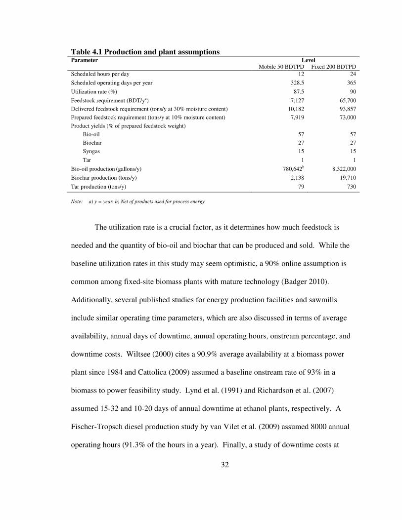
Table 4.1 Production and plant assumptions Parameter Level Mobile 50 BDTPD Fixed 200 BDTPD

Scheduled hours per day 12 24

Scheduled operating days per year 328.5 365

Utilization rate (%) 87.5 90

Feedstock requirement (BDT/ya) 7,127 65,700

Delivered feedstock requirement (tons/y at 30% moisture content) 10,182 93,857

Prepared feedstock requirement (tons/y at 10% moisture content) 7,919 73,000

Product yields (% of prepared feedstock weight)

Bio-oil 57 57

Biochar 27 27

Syngas 15 15

Tar 1 1

Bio-oil production (gallons/y) 780,642b 8,322,000

Biochar production (tons/y) 2,138 19,710

Tar production (tons/y) 79 730

Note: a) y = year. b) Net of products used for process energy

The utilization rate is a crucial factor, as it determines how much feedstock is

needed and the quantity of bio-oil and biochar that can be produced and sold. While the

baseline utilization rates in this study may seem optimistic, a 90% online assumption is

common among fixed-site biomass plants with mature technology (Badger 2010).

Additionally, several published studies for energy production facilities and sawmills

include similar operating time parameters, which are also discussed in terms of average

availability, annual days of downtime, annual operating hours, onstream percentage, and

downtime costs. Wiltsee (2000) cites a 90.9% average availability at a biomass power

plant since 1984 and Cattolica (2009) assumed a baseline onstream rate of 93% in a

biomass to power feasibility study. Lynd et al. (1991) and Richardson et al. (2007)

assumed 15-32 and 10-20 days of annual downtime at ethanol plants, respectively. A

Fischer-Tropsch diesel production study by van Vilet et al. (2009) assumed 8000 annual

operating hours (91.3% of the hours in a year). Finally, a study of downtime costs at

33

hardwood sawmills found an average of 16.7 % downtime at 22 sawmills (Wiedenbeck

and Blackwell 2003).

Under the production assumptions mentioned in table 4.1, the mobile plant would

consume 7,127 BDT of biomass per year and the fixed plant would consume 65,700 BDT

of biomass per year. The feedstock is assumed to be delivered to each plant with a

moisture content of 30%. Therefore, 10,182 tons at the initial moisture content will need

to be delivered to the mobile plant and 93,857 tons to the fixed plant each year. The

feedstock is dried to 10% moisture content to prepare it for pyrolysis in the reactor, so the

prepared annual feedstock requirement for the mobile plant is 7,919 tons and the fixed

plant annual requirement is 73,000 tons.

Based on correspondence with McGill (2009a), both plants are expected to yield

57% bio-oil, 27% biochar, 15% syngas and 1% tar, as a percentage of prepared feedstock

weight. Considering these product yields mobile plant annual production is 780,642

gallons of bio-oil (after a portion is used for process energy), 2,138 tons of biochar, and

79 tons of tar. Fixed plant production is 8.32 million gallons of bio-oil, 19,710 tons of

biochar, and 730 tons of tar.

4.3 Costs

In this section I outline the cost assumptions for both plants. First I address

capital costs and financing, followed by the baseline costs for labor, feedstock acquisition

and handling, energy, maintenance and product delivery. I then outline the calculations

34

used for insurance, taxes and depreciation. The section concludes with a discussion of

the mobile plant move-in and annual relocation costs.

4.3.1 Capital costs and financing

Cost and revenue assumptions are reported in table 4.2. The initial capital

investment for the 50 BDTPD mobile plant mobile pyrolysis plant added up to $3.46

million, including a pyrolysis system cost of $3.42 million (Badger 2009a) and $44,000

for a front-end feedstock loader (Herzog 2009). A spreadsheet software package was

used to calculate financing costs over a 7-year repayment period with equal annual loan

payments8. As suggested by Badger (2009a) and confirmed to be reasonable by Lewis

(2009), the analysis for both plants used an interest rate of 9% for debt financing and a

40% down payment.

8 The initial assumption was a repayment period of 10 years. I subsequently adjusted that to a 7-year repayment based on the advice of a commercial lender in Missoula, MT (Lewis 2009). Lewis suggested that a lender would require a loan period that is shorter than the expected operating life of the plant. Lewis also suggested that an interest rate of 7-8% may be possible as well, though I elected to retain the more conservative rate of 9% in this analysis.

35

Table 4.2 Cost and revenue assumptions Parameter Level Mobile 50 BDTPD Fixed 200 BDTPD

Initial capital investmenta ($) 3,459,000 24,256,000

Pyrolysis system ($) 3,415,000 15,000,000

Loader(s) ($) 44,000 256,000

Other ($) NA 9,256,000

Costs

Down paymentb ($) 1,383,600 9,702,400

Loan paymentc ($) 412,362 2,891,662

Labord ($) 344,137 1,059,240

Feedstockd ($) 143,978 2,978,087

Feedstock loadingd ($) 10,245 23,342

Purchased energyd ($) 68,109 1,595,941

Repair and maintenanced ($) 29,578 333,840

Bio-oil deliveryd ($) 87,588 725,678

Biochar deliveryd ($) 29,158 268,773

Insuranced ($) 45,727 341,257

Annual Mobilizationd ($) 1,632 NA

Move-in and setupb ($) 680 NA

Taxes e ($) varies varies

Revenue Bio-oild ($) 1,063,471 11,337,079 Biochard ($) 290,806 2,680,560 Salvage / end of project revenuef ($) 1,383,600 7,525,600

Notes: a. Sum of ‘pyrolysis system’, ‘loader’, and ‘other’. b. Year 0. c. Years 1-7. d. Years 1-10. e. Tax payments vary each year

due to changes in deductible interest payments and taxable income. Annual tax payments are reported in chapter 6. f. Year

10.

An initial capital investment of 24.26 million was determined for the 200 BDTPD

fixed-site plant9. With a purchase price of $15 million, the largest component of initial

capital investment for the fixed plant was the pyrolysis system. Fixed plant initial capital

investment includes the pyrolysis system and two front end feedstock loaders at a price of

$128,000 each for a total of $256,000 (Carter 2009), as well as allocations for land,

building, site preparation costs, and the additional capital investments required to support

the operation. Additional capital costs for the fixed plant added up to $9.26 million.

9 See Table B.6 in Appendix B for a breakdown of fixed plant initial capital investment.

36

ROI provided an estimate of $10.02 million for the 200 BDTPD system (Badger

2009a). By comparison, the initial capital investment figure used in the Dynamotive

(2009) economic model was $29.3 million, with roughly $20 million of the capital

investment attributed to a 200 BDMT per day pyrolysis system. As noted by Cole Hill

Associates (2004), the lower cost of an ROI facility is explained by differences in

technology that significantly reduce capital and operating costs. The ROI system uses a

mechanical auger reactor (also called a moving bed reactor), as opposed to the fluidized

bed reactor design used by Dynamotive. Therefore, the ROI reactor does not require an

inert gas stream to transport sand or fluidize a bed, thus simplifying the process and

lowering costs (Cole Hill 2004).

The 200 BDTPD ROI facility would consist of four 50 BDTPD modular systems

operating together. Due to the high utilization rate of 90% over 365 scheduled days

chosen for the base case, I assumed that initial capital investment includes the purchase

of five modular 50 BDTPD systems, with only four intended to be used simultaneously.

In this case, each of the five modular units could be taken out of the system periodically

for scheduled maintenance to minimize down time for the overall plant. Taking these

details into consideration, a purchase price of $15 million was assumed for the 200

BDTPD system analyzed in this study, which is approximately the mean of the pyrolysis

system price quoted by ROI (Badger 2009a) and the pyrolysis system price used in the

Dynamotive (2009) study.

I now devote attention to the capital costs in addition to the pyrolysis system at

the fixed site. There are multiple lumber mill sites near Roseburg along Highway 138

that are not in operation due to market conditions in the wood products industry

37

(Lawrence 2009). The Swanson Mill site in Glide, Oregon, owned by Swanson Group,

was suggested as a potential site for the 200 BDTPD pyrolysis plant evaluated in this

study. The financial model assumed that a 20-acre parcel of land at a price of $2

million10 would be necessary to operate the fixed plant (Nelson 2009).

In addition to the pyrolysis system, loader and land costs, I allocated $4 million

for building costs and an additional $2 million for outside improvements including

parking, holding yards, weigh scale, paving, landscaping, and fencing. Finally, $1

million was the assumed cost for non-pyrolysis building contents including office

fixtures, computers, and additional administrative equipment.

It should be noted that there was some uncertainty regarding the portion of initial

investment costs in addition to the pyrolysis system. ROI designs the systems (also

referred to as modules), but they do not design the facilities for the modules and therefore

could not provide a quote for facilities expenses.

The initial capital investment figures were used to determine down payment for

each plant, as well as the annual loan payments that occur in years 1 through 7 of the 10-

year investment period. Financing costs were calculated using the same loan terms for

both the fixed plant and the mobile plant. Assuming 40% of initial capital investment is

paid in year zero of the investment period, a down payment of $1.38 million is paid for

the mobile plant and $9.70 million for the fixed plant. Using the 9% interest rate on

10 This information was obtained by Steve Nelson, Contracting Officer with the Umpqua National Forest, via personal communication with an official at Swanson Group. Swanson Group is a privately held forest products company based in Southern Oregon. It should be noted that the $2 million figure is not an official list price or selling offer, though it is considered a reasonable estimate for the purposes of this study.

38

borrowed funds over a loan period of 7 years, the model includes 7 annual loan payments

of $0.41 million for the mobile plant and $2.89 million11 for the fixed plant.

4.3.2 Labor costs

An hourly wage of $21.5612 was selected for baseline labor costs by accessing the

Quarterly Census of Employment and Wages database on the Bureau of Labor Statistics

website (BLS 2009a). A fringe and benefit rate of 35%13 was added to produce a base

case wage and benefit rate of $29.10 per hour. ROI estimated that the mobile pyrolysis

plant would require three employees during all scheduled operating hours, and a firm

would likely employee two shifts of three employees that work three days on and three

days off (Badger 2009a). With 328.5 scheduled days and three workers working twelve

hours each at a labor cost of $29.10 per hour, the resulting a baseline annual labor was

$344,137.

The fixed plant is a much larger entity than the mobile plant and will therefore

have more specialization and wage variation amongst the employees. Granting that there

will be employees with both higher and lower wages than the mobile plant employees,

this analysis assumed the same average hourly wage and benefit cost of $29.10 per

11 See Appendix B, Table B.7 for a breakdown of fixed plant financing costs. 12 This is based on Average Annual Pay in Douglas County, Oregon in the Forestry and Logging industry. Preliminary 2008 average annual pay per employee for public and private ownership was $54,331 and $35,342, respectively. I calculated the mean of those and converted it to an hourly rate of $21.56, based on 2080 annual hours per employee. 13 I apply a 35% fringe/benefit rate for both the mobile and fixed plant employees in this financial analysis, which is the same rate used by Fight et al. (2006) in the Fuel Reduction Cost Simulator (FRCS). The assumed overhead rate in Farag et al. was 30%, and the benefit rate as a percent of total compensation from the BLS (2009a) online database has varied between 32.3% and 33.1% since 2006 (BLS 2009b). Therefore, 35% is considered appropriate.

39

employee14. Based on the methodology in Farag et al. (2002), I estimated that 17.5 full-

time equivalent (FTE) employees would be required for a 200 BDTPD pyrolysis plant.

With 17.5 employees each scheduled to work 40 hours per week (2080 per year) at wage

and benefit rate of $29.10 per hour per employee, annual labor costs added up to $1.06

million15.

4.3.3 Delivered feedstock and loading costs

Feedstock costs were determined by beginning with biomass stumpage16 and

adding transport and preparation costs. I used a stumpage price of $.09 per ton (Curtis

2009) and assumed the material has an average moisture content of 30% when collected.

Biomass haul cost was calculated based on a trucking cost of $110 per hour (Chung

2009). As the mobile plant will be located in-woods, I assumed the biomass will be

hauled on mostly unpaved forest roads at an average of 10 miles per hour in 12.5 ton

truckloads17. A rate of $7.50 per BDT was also added to account for chipping cost

(Dykstra 2009). Taking each of these feedstock cost parameters into account resulted in

an annual feedstock cost of $143,978 for the mobile pyrolysis plant18.

The fixed plant feedstock costs were calculated using a two-phase haul from the

forest to the plant. A cost of $7.50 per BDT (Dykstra 2009) was allocated for chipping

14 See Appendix C for more details on determining number of employees required for a 200 BDTPD plant and an alternate method of determining average wage and benefit rate. 15 See Table B.8 in Appendix B for a breakdown of fixed plant labor costs. 16 Stumpage is the price charged by a land owner to companies or operators for the right to harvest timber on that land. Stumpage used to be calculated on a "per stump" basis (hence the name). It is now usually charged by tons, board feet or by cubic meters. This analysis is based on a per ton price. 17 The speed and truck capacity for logging roads are based on results from Rawlings et al. (2004). 18 Refer to Table B.1 in Appendix B for mobile plant feedstock cost parameters.

40

the feedstock before it is hauled to a concentration yard located an average of five road

miles from the slash pile. The first phase of the fixed plant feedstock haul is

characterized by the same cost parameters used for the mobile plant feedstock haul—a 10

mile roundtrip at 10 miles per hour in a truck hauling 12.5 tons of biomass at a cost of

$110 per hour. At the concentration yard an allowance of $2.50 per BDT of feedstock

was added to account for re-loading the material into larger trucks (chip vans) that can

haul 25 tons of biomass per truckload. The chip van haul cost was estimated using the

same cost of $110 per hour (Chung 2009), but at a significantly higher average speed of

25 miles per hour. A distance of 45 miles (90 miles roundtrip) is assumed for the second

phase of the biomass haul in the 25 ton chip van. This two-phase biomass haul to the

fixed plant results in a cost of $45.33 per BDT of feedstock, more than twice the

feedstock cost assumed for the mobile plant ($20.20 per BDT). Annual delivered

feedstock costs for the fixed plant added up to $2.98 million19.

Assuming an average feedstock weight of 500 pounds per cubic yard and a 1-yard

capacity bucket on the 262 Skid Steer used at the mobile plant, four loader cycles equal

one ton of feedstock at the initial moisture content of 30%. Operating hours for the

loader were calculated with the understanding the a feedstock weight reduction will occur

after the feedstock is loaded into the system and dried from 30% to 10% moisture

content. Therefore, it was determined that the loader would need to operate 3.1 hours per

day in order to load the annual requirement of 10,182 tons of feedstock at 30% moisture

content. This is equivalent to 7,919 tons after the system dryer reduces the moisture

19 See Table B.9 in Appendix B for a breakdown of fixed plant delivered feedstock costs.

41

content to the 10% level required by the pyrolysis reactor. Taking these factors into

account, total loading costs for the mobile plant added up to $10,326 per year20.

The fixed plant will consume much more feedstock and require a larger wheel

loader with a bucket capable of filling the feedstock metering bin at a faster rate. It was

decided that the 914G wheel loader would need to operate for 6.4 hours per day with a 4

cubic yard bucket to fulfill the annual feedstock requirements of the 200 BDTPD fixed

pyrolysis plant—93,857 tons at 30% moisture content, reduced to 73,000 tons at 10%

moisture content by the system dryer before entering the pyrolysis reactor. Considering

that one loader would reach the end of its useful operating life at roughly five years of

operation under these circumstances, I assumed that two loaders would be purchased at

the beginning of the investment period for the fixed pyrolysis plant. Therefore, the two

loaders could be used interchangeably and remain in service for the lifetime of the

pyrolysis plant. After accounting for fuel consumption and periodic tire replacement and

preventative maintenance, annual loader costs for the fixed plant came to $23,34221.

4.3.4 Process energy consumption and costs

Energy prices tend to have large fluctuation, and the financial performance of a

pyrolysis firm depends on the price and quantity of energy consumed in the production

process. This analysis used 2008 average prices from the Energy Information

Administration (EIA) for propane and electricity to satisfy the thermal and electrical

20 See Table B.2 in Appendix B for the feedstock loading parameters used in this calculation. 21 This figure represents the costs in addition to purchase price and labor costs. Those costs are accounted for in the capital costs and labor costs sections, respectively. See Table B.10 in Appendix B for a breakdown of fixed plant feedstock loading costs.

42

energy requirements, respectively, of the systems. The 2008 West Coast average price of

$2.28 per gallon of industrial propane (EIA 2009a) was assumed to calculate the costs for

the portion of thermal process energy that must be purchased. The Oregon industrial

electricity price of $0.0474 per kWh (EIA 2009b) was used to calculate purchased energy

cost for the fixed plant. It should be noted that some of the process energy calculations

were based on linear projections from ROI. Therefore, they may not reflect the full

extent of energy savings per unit of output that could be expected from scaling up a

facility (Badger 2009a).

For both the mobile and fixed plant financial models, 75% of thermal process

energy was assumed to be provided by syngas produced from the pyrolysis process

(Badger 2009a). The remainder is supplied by purchased propane. However, according

to McGill (2009a), syngas provides a range of 75-125% of the thermal energy needed for

the dryer and pyrolysis reactor. Therefore, the 75% assumption in the baseline analysis is

considered conservative with respect to the financial performance of the two plants.

The thermal energy requirement is 3.22 MMBtu per hour for the mobile plant and

25.78 MMBtu per hour for the fixed plant (Badger 2009a). Propane is purchased to

provide 25% of these energy requirements. This resulted in 8.8 gallons of purchased

propane per operating hour at the mobile plant and 70.5 gallons per hour at the fixed

plant. At $2.28 per gallon of industrial propane (EIA 2009a), the thermal energy costs

for the mobile and fixed plants were $68,109 and $1.27 million, respectively.

All of the electrical energy required for the mobile plant is provided by burning

bio-oil in the flex fuel generator that is integrated with the pyrolysis system. Using bio-

oil for electrical process energy allows the mobile plant to operate without being

43

connected to the electric grid. However, burning bio-oil in a generator with a conversion

efficiency of 30% (S. Badger 2009a) would require 31.25 gallons of bio-oil per hour to

meet the 0.75 MMBtu of electrical energy required each hour. This translated to an

annual diversion of 122,188 gallons of bio-oil from the market, with an estimated market

value of $166,456 at the baseline delivered price of $1.36 per gallon. The same quantity

of electrical energy could be purchased from the grid for approximately $40,739 at a

price of $0.0474 per kWh, the electricity price assumed for the fixed plant. Therefore,

under these assumptions the mobile plant would sacrifice $125,717 in annual revenue in

order to operate off-grid. That opportunity cost is accounted for in the mobile plant

revenue section by reducing the quantity of bio-oil for sale.

Considering the thermal and electrical energy parameters mentioned above, the

annual purchased energy cost amounted to $68,10922 for the mobile plant. This cost was

completely attributed to propane purchased to provide the 25% of thermal process energy

not met by syngas.

Electrical energy for the fixed plant was assumed to be purchased entirely from

the electric grid (McGill 2009b)23 at a rate of $0.0474 per kilowatt-hour (kWh) (EIA

2009). With 876 kWh purchased each operating hour, annual electrical energy costs for

the fixed plant added up to $0.33 million, which brought the total fixed plant energy costs

to $1.60 million each year.

22 Energy costs for the mobile plant are delineated in Table B.3 of Appendix B. 23 See Table B.11 of Appendix B for a breakdown of fixed plant energy consumption and costs.

44

4.3.5 Repair and maintenance costs

Repair and maintenance (R&M) costs were provided by ROI for both the mobile

and fixed plants. ROI has not previously manufactured plants as large as the 50 and 200

BDTPD plants considered in this analysis. Therefore, the R&M costs are projections

based on smaller plants as opposed to actual costs.

The mobile plant is expected to have annual repair and maintenance costs of

$29,578 for the pyrolysis system, which includes $1400 in lube and oil costs for the flex

fuel generator used to supply electrical process energy (Badger 2009a).

Badger (2009a) provided an annual repair and maintenance estimate for the fixed

plant that was equal to 1.5% of the quoted pyrolysis system purchase price. I calculated

R&M costs based on 1.5% of initial capital investment figure used in this study (not

including land), using the increased pyrolysis system cost described in section 4.3.1.

Annual R&M costs for the fixed plant then came to $330,840 (Badger 2009a).

4.3.6 Product delivery costs

Costs for bio-oil and biochar delivery are important factors regarding the financial

performance of a pyrolysis plant. Figure 4.1 displays the expected market locations for

bio-oil and biochar produced at the mobile and fixed pyrolysis plants. The assumed

market for bio-oil is Portland, Oregon, and biochar is expected to be sold within a 2.5

hour average haul distance from each plant.

Product delivery costs are addressed in sections 4.3.6.1, 4.3.6.2 and 4.3.6.3. I

begin by discussing the bio-oil delivery costs and follow with delivery costs for the

biochar and tar produced at the mobile and fixed pyrolysis plants.

45

4.3.6.1 Bio-oil delivery costs

Cost estimates for delivery of bio-oil to selected end-use markets were obtained

from a fuel trucking firm in Roseburg (Dirksen 2009). As shown in table 4.3, delivery

cost per gallon depends on trucking route and the size of fuel truck used. Delivery cost

decreases as fuel truck size increases and delivery cost increases as haul distance

increases. While the trucking route and size of truck will vary depending on mobile plant

location, I have attempted to balance out the costs for the base case by choosing to use

the cost estimates for hauling to Portland, the longest trucking route, and the largest fuel

truck with a 9000 gallon capacity. Therefore $.1122 per gal is the baseline average fuel

delivery cost for the mobile plant. With a projected bio-oil sales volume of 780,642

gallons per year, annual delivery costs were estimated to be $87,588 for the mobile plant.

Table 4.3 Dirksen & Sons bio-oil delivery estimate (cents per gallon) Small bobtail (2000

gallon) Large Bobtail (3500

gallon) Transport (9000

gallon)

Lemolo Lake junction to Roseburg (79 mi)

.1717 .1017 .0467

Lemolo Lake junction to Eugene (150 mi)

.2417 .1456 .0760

Lemolo Lake junction to Portland (251 mi)

.3272 .2172 .1122a

Glide to Roseburg (16 mi)

.1217 .0717 .0217

Glide to Eugene (88 mi) .1917 .0956 .0456 Glide to Portland, OR (195 mi)

.2872 .1872 .0872b

Source: Dirksen (2009)

Notes: a. Baseline cost used for mobile plant bio-oil delivery

b. Baseline cost used for fixed plant bio-oil delivery

46

Figure 4.1 Market locations for bio-oil and biochar

Source: Page-Dumroese (2010)

Bio-oil delivery costs for the fixed plant were based on transport from Glide to

Portland in a 9000 gallon fuel truck. With 8.32 million gallons of bio-oil to be sold each

year and transport costs of $0.0872 per gallon, annual bio-oil delivery costs for the fixed

plant came to $725,67824.

24 See Table B.12 in Appendix B for a breakdown of fixed plant bio-oil delivery costs.

Bio-oil market

Biochar

market

47

4.3.6.2 Biochar delivery costs

Biochar is assumed to be sold into smaller markets within 2.5 hours by road from

the mobile pyrolysis plant, and a five-hour average truck rental was estimated for each

27.5 ton biochar delivery. A $70 per hour cost for delivery results in an average cost per

truckload of $375 (Whitaker 2009). These parameter levels produced an annual biochar

delivery cost of $29,15825 for the mobile plant.

The fixed plant located in Glide, Oregon will produce approximately 19,710 tons

of biochar for market annually. As the fixed-site pyrolysis plant is located closer to

Roseburg, a likely market center for biochar, a significant portion of the biochar will

likely have a shorter and less costly haul to market than the biochar produced at the

mobile plant. However, due to the significantly larger quantity of biochar that is

produced, it is likely that a portion of the biochar will need to be transported longer

distances in order to be absorbed into the market. I assumed that these tradeoffs cancel

each other out. Therefore, 5 hours was the assumed roundtrip trucking time to bring

biochar to market from the fixed plant, the same baseline haul time used for the mobile

plant. With 717 truckloads of biochar transported to market per year, the annual cost for

biochar delivery from the fixed plant comes to $268,77326.

4.3.6.3 Tar delivery costs

As reported in table 4.1, up to 1% of the biomass may be converted to “tar” in

ROI pyrolysis systems (McGill 2009a). Based on 1% of prepared feedstock weight, the

25 See Appendix B, Table B.5 for a breakdown of mobile plant biochar delivery costs. 26 See Appendix B, Table B.13 for a breakdown of fixed plant biochar delivery costs.

48

mobile plant would produce 79 tons of tar each year, and the fixed plant would produce

730 tons. This financial model accounts for tar production by decreasing the bio-oil and

biochar outputs from 57.5% and 27.5% to 57% and 27%, respectively.

Further research is needed on the characteristics of pyrolysis tar to determine if it

is a product that could be sold for revenue or a waste product that generates disposal

costs. Due to the uncertainties regarding the chemical makeup of the tar and its

suitability for value-added products, it is considered revenue neutral in the analysis. For

this study, I assume that tar is sold to end users at a price equal to the transportation cost.

Therefore, no net change in cash flow is generated.

4.3.7 Insurance costs

The insurance costs for both plants were based on correspondence with an

insurance provider in Roseburg, Oregon (Wood 2009). Annual premiums were

calculated according to the value of assets and the annual gross revenue of the firm.

Liability insurance premiums were calculated as 1.5% of gross revenue27. Property

insurance premiums were based on 0.4% of asset value for buildings and 0.7% of the

building contents value. As no buildings are required for an in-woods mobile plant,

property insurance was calculated at 0.7% of the pyrolysis system cost. Finally, an

annual cost of $1200 was included for Directors and Officers Liability Insurance (D&O)

for each system (Wood 2009). D&O is intended to cover legal expenses for alleged

“wrongful acts” committed by directors and officers of the company.

27 An insurance agent in Roseburg (Wood 2009) suggested a rate of 1.875% of revenue to calculate annual liability insurance premiums, and ROI suggested 1% of revenue. Therefore, I elected to use a rate between those two, but slightly closer to the higher cost estimate.

49

The annual property insurance premium for the mobile plant was $24,213 and the

annual liability insurance premium is$20,314. Including $1,200 D&O, the total annual

insurance cost for the mobile plant added up to $45,727.

For the fixed plant, annual property insurance for the building was $16,000, and

$113,792 for the contents of the building. Calculated according to 1.5% of gross

revenue, another $210,265 per year was included for liability insurance. By adding these

insurance cost components to the $1,200 allocation for D&O, total annual insurance cost

for the fixed plant came to $341, 257.

4.3.8 Taxes and depreciation

For both the 50 and 200 BDTPD pyrolysis plants, taxes paid on net cash flow

(minus depreciation) were incorporated to determine NPV, IRR, and Payback Period.

The model developed for this project assumed that federal taxes are paid according to

Internal Revenue Service (IRS) Form 1120, Schedule J28, and a $10 minimum tax plus a

6.6% corporate excise tax is paid to the state of Oregon according to Form 20, the Oregon

Corporate Excise Tax Return29. Taxable income and taxes paid vary each year due to the

changing proportion of the loan payments that are attributed to principal and interest. As

portion of the loan payment attributed to interest decreases during the loan repayment

period, the tax bill increases because less interest is deducted from gross income to

calculate taxable income.

28 See Appendix D for the federal corporation tax schedule applied in this analysis 29 Oregon taxes were calculated based on compliance with 2008 tax laws. New legislation that would increase the minimum tax, income and excise taxes for corporations was pending at the time of this analysis.

50

Straight line depreciation of capital over the useful operating life of ten years is

assumed for the purpose of reporting taxable income to the IRS. It should be noted that

no special financing and grant programs or accelerated depreciation30 are used in the

analysis, nor are production credits or employment credits. Further investigation of these

opportunities would be warranted as a firm develops a business plan and seeks debt

financing for a pyrolysis plant. A firm could expect increased financial performance

upon the passing of preferential biomass energy legislation and if favorable depreciation

and special financing programs are incorporated.

4.3.9 Mobile plant initial mobilization and annual relocation costs

Initial mobilization costs are specific to the mobile plant that will operate in-

woods near forest biomass stocks generated from thinning and restoration activities. The

purchase price for the pyrolysis system includes delivery to Roseburg, Oregon, and the

system is permanently mounted on two 53-foot lowboy trailers (Badger 2009c).

Mobilization costs include a $68 per hour per truck rental to transport the pyrolysis

system to the processing locations (Whitaker 2009). The model includes rental of two

trucks for five hours for initial mobilization, resulting in an initial mobilization cost of

$680.31

30 Modified Accelerated Cost Recovery System (MACRS) is the system used in the IRS tax code to depreciate property purchased after 1986 on an accelerated basis. This encourages business investment by lowering the tax burden of a business during the early years of the investment period. 31 This analysis does not identify the initial or subsequent specific locations for the mobile pyrolysis plant, though a 5-hour roundtrip haul is assumed to be reasonable for initial mobilization into the study region. An additional hour of truck rental is included for relocation to account for time to move the two trailers from one location to another.

51

I assume the mobile unit is relocated twice per year in order to move closer to

available biomass to maintain an average roundtrip feedstock haul of no more than ten

miles. An additional six-hour rental of two trucks at a cost of $68 per hour per truck is

included each time the system is relocated (Whitaker 2009). Relocation cost includes

two moves per year at $816 per move, for a total annual relocation cost of $1632 for the

mobile plant.

It is assumed that three employees will spend eight hours breaking down the

equipment and eight hours setting it up at each new location (Badger 2009c). The break

down and set up labor for the employees is accounted for in the annual employment costs

section. The forgone production of bio-oil and biochar caused by equipment downtime

during the move is an opportunity cost of relocation. I account for this by lowering the

baseline scheduled operating days per year from 328.5 to 325.8 to reflect two moves per

year at 16 hours (1.33 operating days) per move.

4.4 Benefits

This section outlines the annual revenue sources for the mobile and fixed

pyrolysis plants, starting with the revenue from bio-oil and concluding with biochar

revenue. The financial analysis includes revenue equal to the salvage value of each plant

at the end of the 10-year operating life.

According to ROI, their systems produce 55-60% bio-oil, 25-30% biochar and

15% syngas, as a percentage of feedstock weight (Badger 2009a). I assume that average

product output is the midpoint of those output ranges, with .5% subtracted from both bio-

oil and biochar to account for 1% tar. McGill (2009a) added that the percentage of

52

syngas has negligible variation and the percentages of bio-oil and biochar vary with a

direct tradeoff relationship (e.g., 1% more bio-oil means 1% less biochar.

Bio-oil accounts for the majority of the revenue for each plant, with 57% of the

feedstock weight coming out in liquid form. Biochar is expected to provide significant

income as well, with 27% of the feedstock weight coming out in solid form. The

remainder of the feedstock weight becomes syngas which is used for process energy, and

tar which is mentioned above.

4.4.1 Bio-oil revenue

A representative of Dynamotive, a Canadian pyrolysis firm headquartered in

British Columbia, suggested setting bio-oil delivered price equivalent to No. 2 fuel oil on

a price per unit of energy basis with a 10% discount32 (Bouchard 2009). The 10%

discount is provided as an incentive to switch to bio-oil and pay for equipment upgrades

necessitated by the adverse chemical properties of bio-oil. The necessary upgrades may

include changing burners, nozzles and storage containers to stainless steel to avoid

corrosion. Equation 4.1 includes the valuation method for bio-oil used in this study,

��� � ��� � ��

���� 90% (4.1)

32 By contrast, ROI values its product based on a 5% discount per unit of energy of the fossil fuel it is replacing (Badger, S. 2009a). This analysis uses the more conservative pricing method that discounts bio-oil by 10%.

53

where Pbo is the price of bio-oil, Pfo is the price of No. 2 fuel oil, ECbo is the per gallon

energy content of bio-oil, and ECfo is the per gallon energy content of No. 2 fuel oil.

Based on a fuel oil price of $2.64 per gallon33 and accounting for differences in energy

content and a 10% discount, a delivered price of $1.36 per gallon of bio-oil is used in this

analysis. With 2,420 gallons of bio-oil for sale each operating day, the mobile plant is

expected to generate $1.06 million in annual revenue from bio-oil sales.

Bio-oil delivered price is based on substitution for No. 2 fuel oil and the

methodology in equation 4.1. The bio-oil yield per ton of feedstock, weight per gallon,

energy content per gallon, and No. 2 fuel oil price all impact the delivered price of bio-

oil. With an average of 22,800 gallons of bio-oil produced per operating day, the fixed

plant is expected to sell 8.32 million gallons per year. This translates to annual revenue

of $11.34 million in bio-oil sales from the fixed plant.

4.4.2 Biochar revenue

Biochar values and selling prices tend to vary widely. ROI suggested that values

range from $60 to $260 per ton depending on the market the biochar is sold in (Badger

2008). The Dynamotive (2009) analysis assumed a value of $150 per metric ton

(equivalent to $136 per US ton) based on the heating value of biochar compared to coal,

adding that the value could be much higher if it were used for soil improvement and

carbon sequestration. Another biochar producer suggested that the soil amendment

values for biochar range from $100-$500 per ton, and are likely to rise as carbon markets

33 This was the average No. 2 fuel oil price during the 24-month period from September 2007 through August 2009 (EIA 2009a).

54

mature and biochar carbon offset projects are developed (Fournier 2009). Miles (2009)

suggested a wholesale biochar price of $200 per ton. Finally, a case study on ‘Large-

scale bioenergy and biochar’ by Joseph and Watts (2009) assumes that biochar is sold in

horticultural markets for $120 to $180 per metric ton.

After reviewing these prices, a baseline delivered price of $136 per ton34 was

chosen for this study. It was assumed that biochar is sold into regional horticultural

markets as a soil amendment, though it could also be sold into energy markets if

sufficient demand is derived. With 0.27 tons of biochar produced per ton of feedstock

(McGill 2009a), the mobile plant is expected to yield 6.56 tons of biochar per operating

day. This translates to $290,806 in annual revenue from biochar sales. Biochar revenue

for the fixed plant is also based on a delivered selling price of $136 per ton. With 54 tons

produced per day, annual fixed plant biochar revenue amounted to $2.68 million.

4.4.3 Salvage revenue

The financial benefit from salvage revenue was assumed to be realized at the end

of the 10-year investment period for both the mobile and fixed pyrolysis plants. Badger

(2009a) suggested a salvage value equal to 10% of the initial purchase price. For the

mobile plant, salvage value in year 10 is equal to 10% of initial capital investment, or

$345,900.

For the fixed plant, salvage value was calculated as 10% of the pyrolysis system

purchase price plus the purchase price of the two loaders, or $1.53 million. Revenue

34 Equivalent to $150 per metric ton.

55

from the sale of the land and buildings at the fixed plant is equal to their original

purchase price in the discounted cash flow model. As a real (net of inflation) discount

rate is used, this implies that the value of the land and buildings are assumed appreciate

in value at a rate equal to the inflation rate during the investment period. Therefore, a $6

million financial benefit was added to the $1.53 million salvage value for a total of $7.53

in salvage and “end of project” revenue at the fixed plant.

56

Chapter 5

Financial analysis methods

5.1 Introduction

A discounted cash flow analysis (DCFA) for a 50 BDTPD mobile plant and a 200

BDTPD fixed-site plant in southwest Oregon was performed in the MS Excel spreadsheet

software package. Using the above assumptions and cost and revenue data from chapter

4, multiple financial performance measures were highlighted for the baseline scenario.

Sensitivity analyses were performed around several key variables to determine how

changes in their levels affect the Net Present Value (NPV) of each system. I rely on

Dayanda et al. (2002) and Boardman et al. (2006) to describe the discounted cash flow

analysis (DCFA) method and evaluate financial performance of the pyrolysis

investments.

The chapter begins with an overview of DCFA and NPV, including a description

of the variables and equations used to measure financial performance in this model. The

internal rate of return and payback period performance measures are then discussed.

Finally, the sensitivity analysis and breakeven analysis methods are described.

5.2 Discounted cash flow analysis and net present value

In DCFA, after tax cash flows are “discounted” in order to reflect the preference

for current consumption over future consumption. A discount rate is used to convey this

preference and discount future cash flows to present value. A real (net of inflation)

discount rate of 7% was used in this study. The appropriate discount rate varies from one

57

firm or entity to another. The Dynamotive (2009) analysis used a 6% discount rate

(referred to as “hurdle rate”) and Ringer et al. (2006) used a 10% discount rate, while the

USDA Forest Service typically uses a 4% discount rate for investments. All cash flows

for the life of a project, both positive and negative, are summed in terms of present value

in order to arrive at NPV for each project.

Most of the cost items are shared by both the fixed and mobile plant. Table 5.1

displays the cost and revenue variables described in sections 4.2 and 4.3. The energy cost

variable, Ent, includes only the purchased propane used to satisfy 25% of the required

thermal energy for the mobile plant, as bio-oil will be used for 100% of the mobile plant

electrical energy. For the fixed plant, the energy cost variable includes purchased

propane for 25% of the required thermal energy and purchased electricity to provide

100% of the required electrical energy. The move-in/setup and annual mobilization and

costs, denoted by Mobt, are only incurred by the mobile plant.

58

Table 5.1 List of cost and benefit variables Variable Variable description

Costs: Fint down payment (year 0) + loan payment (years 1-7) Lt labor cost Feedt prepared feedstock cost Loadt loading costs Ent purchased propane + purchased electricity cost Maintt repair and maintenance cost Delt bio-oil + biochar delivery cost Inst insurance cost Taxt property taxes + income and excise taxes Mobt move-in/setup (year 0) + annual mobilization

(mobile plant only)

Benefits: ���� delivered price of bio-oil

���� quantity of bio-oil sold

��� delivered price of biochar

��� quantity of biochar sold

Salvt salvage revenue + sale of additional assets (year 10)

Equations 5.1 and 5.2 summarize the costs and benefits that were ascertained for

each plant and used to calculate NPV with the subsequent equations. As shown in

equations 5.3 through 5.5, NPV is the present value of the benefits minus the present

value of the costs for a project, where r is the discount rate and t is the year in which the

costs (C) and benefits (B) occur. The project length is 10 years, so t varies from 0 to 10.

The NPV model is the primary model to be used as a decision rule for investment in a

project (Dayanda 2002). However, it is wise to use additional measures to check the

validity of or add robustness to the decision suggested by the NPV measure. Generally

speaking, firms should reject projects that have a negative NPV and accept projects with

a positive NPV. This does not take into account resource constraints such as access to

funds for initial capital investment. Also, when weighing multiple projects, whether the

projects are mutually exclusive is an important factor. In some situations adoption of one

59

project precludes adoption of another project, and in others, multiple projects can be

adopted provided that they each exhibit a positive NPV.

When interpreting NPV, it is important to realize that an NPV of zero does not

imply zero profit. It simply means that the project is expected to generate returns equal

to the discount rate, which is also assumed to be the minimum acceptable rate of return

(MAR) for the investor. Therefore, setting an appropriate discount rate is very important

in project appraisal, as it is a major factor in determining whether a project will be

undertaken. A higher discount rate decreases the likelihood that a project will be

accepted, while the opposite is true of a lower discount rate. Positive NPV indicates

returns above and beyond the MAR and can be thought of as the additional wealth that

will be generated by undertaking the project, relative to the next best alternative.

�� � ���� � �� � ����� � ����� � ��� � ���� � �

!�"� � #�$� � %�&� � ��'� (5.1)

(�)���� � ��

�� � ��� � ��

� � *�"+� (5.2)

�,-(. � ∑�0

-123.014�)4 (5.3)

�,-�. � ∑0

-123.014�)4 (5.4)

5�, � �,-(. 6 �,-�. (5.5)

Both the mobile and fixed pyrolysis plants exhibit a positive NPV in the baseline

analysis. The mobile plant NPV is $35,748, and the fixed plant has an NPV of $9.68

million. The fixed plant does require a much larger initial capital investment, so it is

60

helpful to look at additional performance criteria prior to ranking the projects. In

addition to NPV I also consider the internal rate of return (IRR) and payback period to

evaluate the financial performance.

5.3 Internal rate of return

Internal Rate of Return (IRR) is the discount rate that sets NPV to zero in

equation 4.1 (Boardman et al. 2006). Therefore, IRR greater than the discount rate

corresponds to positive NPV and an IRR less than the discount rate corresponds to

negative NPV. The IRR measure can be used to evaluate the financial performance of a

single project, but it can be misleading if used to compare multiple projects. The

decision rule for IRR is to accept projects with an IRR greater than or equal to the chosen

discount rate. Thus, the 7.4% mobile plant IRR shows that the mobile plant project is

acceptable under the IRR criterion, though not by much. On the other hand, the 20.9%

fixed plant IRR indicates a more attractive investment that would be acceptable to an

investor requiring a high 20% return.

There are drawbacks to using IRR when comparing projects of different size. For

example, a small project with a high IRR is not necessarily preferable to a larger project

with a low IRR, as the larger project could still generate greater value for the firm.

However, as Dayanda et al. (2002) mention, decision-makers often deal with ‘rates of

return’, and therefore IRR is helpful because it can be thought of as the rate of return on

an investment. Project analysts often use IRR as a complement to NPV when reporting

financial performance to stakeholders. I used the IRR function available in MS Excel,

which iteratively adjusts the discount rate until NPV equals zero.

61

5.4 Payback period

Payback period refers to the time it takes for non-discounted cumulative revenue

to exceed the cumulative costs associated with a project. The decision rule for this

measure is to choose the project with the shortest payback period, though results should

be interpreted with caution. In this case, the fixed plant has a payback period of six years

and the mobile plant payback period is nine years. Therefore, the payback period

measure further supports the superior financial performance of the fixed plant indicated

by the NPV and IRR measures.

Using payback period as a stand-alone financial performance measure is generally

discouraged (Dayanda et al. 2002; Boardman et al. 2006), though it may be helpful as an

addition to NPV and IRR. It may be especially relevant to someone with a very short

time horizon for an investment, particularly a foreign investment with considerable

perceived risk. A downside to reporting payback period is that cash flows are not

discounted, and therefore the time value of money is not taken into account (Dayanda et

al. 2002). For example, if the payback period for a proposed project is six years, but the

vast majority of the “payback” occurs in the sixth year, this is quite different (and less

desirable) than a project with a payback period of six years where an equal portion of the

investment is “paid back” each year. Also, payback period does not take into account

what happens during the remaining life of a project after the investment is paid back.

There could be cleanup costs associated with plant decommissioning at the end of a

project, which would decrease the attractiveness of the investment. Or, there could be

significantly higher net cash flows after payback occurs, which would increase the

62

attractiveness of the investment. Therefore, while payback period can be helpful as an

addition to other financial performance measures, giving too much consideration to

payback period may lead to flaws in the ranking of potential projects.

5.5 Sensitivity analysis

Several cost variables were varied by plus and minus ten and thirty percent. The

range of plus and minus thirty percent was chosen by examining the plausible amount of

variation in each parameter. According to the US Bureau of Labor Statistics, average

annual pay in the forestry and logging industry in Douglas County, Oregon was $54,331

for government ownership and $35,342 for private ownership (BLS 2009). After

converting these to hourly wages and adding the fringe and benefit rate of 35%, we see

that labor costs for public ownership are twenty-one percent higher than the baseline rate

of $29.10 per hour. Labor costs for private ownership are 21% lower. Therefore, the

range of plus and minus ten and thirty percent variation from the baseline should

adequately capture the range of plausible labor costs.

A major determinant of feedstock cost is the haul distance to the pyrolysis plant.

For the mobile plant, a ten mile roundtrip haul distance and delivered cost of $20.20 per

BDT has been assumed for the baseline analysis. Allowing the baseline cost assumption

to vary by plus and minus ten and thirty percent produces a cost ranging from $14.14 per

BDT to $26.26 per BDT. A roundtrip haul of 5.2 miles would produce the lower bound

cost and a haul of 14.8 miles would produce the upper bound cost. It is unlikely that a six

month feedstock supply of thinning from forest restoration and thinning practices would

be available within an average haul of less than 5.2 miles for the lower bound. The upper

63

bound price is similar to the rate being paid in Roseburg as of fall 2009 for hog fuel (Pine

2009). As one of the goals of mobile pyrolysis is to decrease haul costs and the overall

cost of feedstock, it is reasonable that the upper bound haul distance should not produce a

feedstock cost that is higher than the feedstock cost being paid by cogeneration facilities

in Roseburg.

5.6 Breakeven analysis

Bio-oil and biochar are the two products that generate annual revenue for the

project, so it was logical to conduct a sensitivity analysis on the delivered price of each. I

believe there is greater uncertainty in the prices of these good and thus consider larger

pricing variations for the revenue parameters than the cost parameters mentioned above.

This was done for two reasons—first, to encompass the range of recent observed prices

for No. 2 fuel oil, which is used to calculate bio-oil price according to equation 4.1.

Next, to reflect the uncertainty associated with selecting the appropriate baseline

delivered prices for the revenue generating products of pyrolysis. Therefore, sensitivity

analyses were conducted for baseline prices plus and minus thirty and fifty percent for

bio-oil. This produced bio-oil delivered prices ranging from $.68 to $2.05 per gallon

which correspond to $1.36 to $3.95 per gallon for No. 2 fuel oil. No. 2 fuel oil prices

fluctuated between $1.55 and $4.02 during the 24-month period that ended with August

200935.

35See Appendix E for a figure displaying No. 2 fuel oil prices from September 2007 through August 2009.

64

Biochar prices were also varied by plus and minus ten, twenty and fifty percent,

as well as the extreme prices of $0 and $500 per ton. A value of $0 per ton was included

to represent a scenario where the biochar is used as a soil amendment in the areas the

biomass feedstock was sourced from. In this case, the biochar delivery cost would

become the cost associated with applying biochar back to the land. It has been suggested

that the impacts of climate change will drive up the price of biochar over time (Fournier

2009), and therefore the high value of $500 per ton was also included.

Breakeven parameter levels were identified by using the “goal seek” function in

MS Excel. Goal seek allows the user to find the level of one parameter required to

change another variable, the goal variable, to a level of interest. In this case, the function

was used to identify the value of certain parameters that would set NPV to zero. When

NPV is zero, the investment breaks even by delivering an IRR equal to the discount rate.

The discount rate is assumed to be the minimum acceptable rate of return (MAR) for the

investor, or equal to the rate of return that could be earned on the next best alternative.

Therefore, breakeven parameter levels are helpful in examining each variable to identify

the level required for the investment to be undertaken.

65

Chapter 6

Financial performance of mobile and fixed-site pyrolysis plants

6.1 Introduction

In this chapter I present the baseline financial performance results of the mobile

and fixed pyrolysis plants under the baseline assumptions described in the previous

chapter. The NPV, IRR, and payback period measures are reported for each plant. The

chapter concludes with a discussion of the financial tradeoffs between mobile and fixed

pyrolysis operations.

6.2 Mobile plant financial performance

Table 6.1 details the cash flow and tax burden projections for an in-woods 50

BDTPD mobile fast pyrolysis plant in southwest Oregon under the assumptions described

in the preceding chapter. Year zero can be thought of as the instant before year one

begins, including the costs incurred prior to the plant commencing operation. This

includes a large capital outlay for down payment and initial mobilization costs. Revenues

are then constant from year one until the last year of operation, which includes additional

revenue equal to the salvage value of the plant. Taxable income increases each year as

the loan is paid down and a smaller portion of the loan payment is allocated to tax-

deductable interest. Cash flow and tax due greatly increase during the last three years of

operation. This is due to the loan being paid in full which means there are no interest

payments to deduct from gross revenue to calculate federal taxable income.

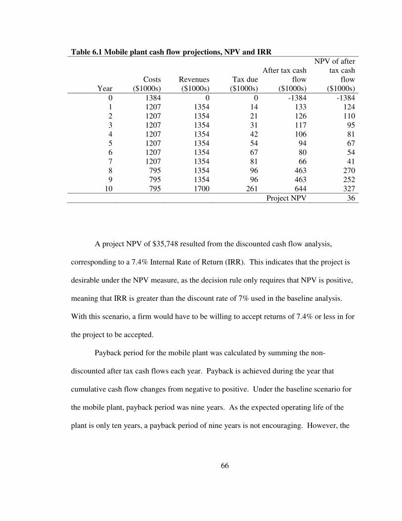
66

Table 6.1 Mobile plant cash flow projections, NPV and IRR

Year Costs

($1000s) Revenues ($1000s)

Tax due ($1000s)

After tax cash flow

($1000s)

NPV of after tax cash

flow ($1000s)

0 1384 0 0 -1384 -1384 1 1207 1354 14 133 124 2 1207 1354 21 126 110 3 1207 1354 31 117 95 4 1207 1354 42 106 81 5 1207 1354 54 94 67 6 1207 1354 67 80 54 7 1207 1354 81 66 41 8 795 1354 96 463 270 9 795 1354 96 463 252

10 795 1700 261 644 327

Project NPV 36

A project NPV of $35,748 resulted from the discounted cash flow analysis,

corresponding to a 7.4% Internal Rate of Return (IRR). This indicates that the project is

desirable under the NPV measure, as the decision rule only requires that NPV is positive,

meaning that IRR is greater than the discount rate of 7% used in the baseline analysis.

With this scenario, a firm would have to be willing to accept returns of 7.4% or less in for

the project to be accepted.

Payback period for the mobile plant was calculated by summing the non-

discounted after tax cash flows each year. Payback is achieved during the year that

cumulative cash flow changes from negative to positive. Under the baseline scenario for

the mobile plant, payback period was nine years. As the expected operating life of the

plant is only ten years, a payback period of nine years is not encouraging. However, the

67

fact that payback does occur during the operational life of the plant means that the project

should not necessarily be dismissed.

6.3 Fixed plant financial performance

The before and after tax cash flow projections of a fixed 200 BDTPD plant

located in Glide, Oregon are summarized in table 6.2. Taxable income and tax due

exhibit an upward trend, with a significant increase at the end of the investment period

due to diminishing tax-deductable interest payments and the addition of salvage revenue

at the end of year ten.

Table 6.2 Fixed plant cash flow projections, NPV and IRR

Year Cost

($1000s) Revenue ($1000s)

Tax due ($1000s)

After tax cash flow ($1000s)

NPV of after tax cash

flow ($1000s)

0 9702 0 0 -9,702 -9,702 1 10,428 14,018 1,562 2,028 1,895 2 10,428 14,018 1,620 1,970 1,720 3 10,428 14,018 1,683 1,907 1,556 4 10,428 14,018 1,752 1,838 1,402 5 10,428 14,018 1,827 1,763 1,257 6 10,428 14,018 1,908 1,682 1,121 7 10,428 14,018 1,997 1,593 0,992 8 7,536 14,018 2,094 4,387 2,554 9 7,536 14,018 2,094 4,387 2,386

10 7,536 21,543 5,156 8,851 4,500

Project NPV 9681

68

Investment in the fixed plant project appears to be quite attractive, with an NPV

of $9.68 million and an IRR of 20.9%. This implies that a potential investor would see

this project as worthy of investing in, provided that the investor’s MAR is less than 21%.

After a large initial cash outlay at the start of a project, it often takes several years for a

project to exhibit positive cumulative cash flow. This is the case with the fixed pyrolysis

plant, even though it exhibits healthy annual after tax cash flow. In the baseline scenario

for the fixed plant, cumulative cash flow changes from negative to positive in the sixth

year of operation, so the payback period is six years.

6.4 Sensitivity analysis

Next I present the results of the sensitivity analysis relative to the baseline results

already mentioned in the previous section. The sensitivity analysis was performed by

allowing variation in some of the key cost and revenue assumptions of the model. If the

NPV rule continues to be satisfied under different scenarios then the results of the model

would provide robust support of the financial feasibility of these pyrolysis plants. I

present the effects of variation of those variables to which the financial feasibility is most

sensitive.

I begin by focusing on the mobile plant sensitivity analysis and follow with the

fixed plant. For each plant, I first discuss several important cost variables. Then, the

impact of variation in bio-oil and biochar delivered prices on financial performance is

addressed, with break even prices determined. The NPV measure is the dependent

variable in each scenario of the sensitivity analysis.

69

6.4.1 Mobile plant sensitivity analyses

The baseline NPV for the mobile plant is positive and therefore acceptable under

the NPV decision rule. However, at just $35,748, the project NPV is only marginally

acceptable at a 7% discount rate. Adjusting the level of any variable that impacts

financial performance could quickly change the investment outlook of the project from

acceptable to undesirable. Following is a discussion of the sensitivity of mobile plant

financial feasibility to several cost variables and the two revenue variables—bio-oil and

biochar prices.

Varying the level of initial capital investment was found to have a large effect on

NPV for the mobile plant, as shown in section A.1 of Appendix A. Increasing the mobile

plant initial capital investment by 30% from $3.46 million to $4.50 million decreased

NPV from $35,748 to -$815,462. On the contrary, if the initial capital investment were

30% lower, the mobile plant returns would be significantly higher at $735,995.

Of the annual operating costs in figure 6.1, NPV of the mobile plant project is

most sensitive to labor costs. Of the selected cost variables displayed in the figure, the

next most important variable is feedstock cost, followed by interest rate on borrowed

funds, bio-oil delivery cost, and finally, biochar delivery cost.

70

Figure 6.1 Mobile plant NPV sensitivity to several important cost variables

Labor costs represent the largest share of annual costs for the mobile plant.

Therefore, changes in wage and benefit rate used to calculate labor costs have a dramatic

effect on NPV and those costs deserve significant attention. It is worthwhile to further

examine the method used to determine baseline wages and labor hours needed. An

interested party could look at the baseline wage and benefit rate and investigate how that

rate may change in real (inflation adjusted) terms over the 10-year operating period of the

plant by consulting the Bureau of Labor Statistics website to look at trends in forestry and

natural resource professions. By using a real discount rate, wages are implicitly assumed

to rise with inflation during the investment period. However, if wages in this

employment sector rise more rapidly than the rate of inflation, the baseline wage and

-$500,000

-$400,000

-$300,000

-$200,000

-$100,000

$0

$100,000

$200,000

$300,000

$400,000

$500,000

-30% -10% Base case +10% +30%

NP

V o

f af

ter

tax

cash

flo

ws

Change in parameter level

Labor costs

Feedstock Cost

Interest rate on

borrowed funds

Bio-oil delivery cost

to market (Portland,

OR)

Biochar delivery cost

to market

71

benefit rate used in this analysis would have underestimated labor costs and led to overly

optimistic financial performance results.

The required labor to operate the plant should be carefully considered as well. If

further research leads to a belief that the projected amount of labor hours are more than

enough, an investor can have more confidence in proceeding with the project. If further

investigation suggests that labor costs and required labor were estimated too

optimistically in the base case with respect to financial performance, caution in

proceeding with the project should be exercised.

Feedstock costs are the next cost variable to investigate, though they have

significantly less impact on the financial performance of the mobile pyrolysis plant than

labor costs. A prospective stakeholder should revisit the feedstock cost estimation

method discussed in section 4.3.2. An average feedstock haul of five miles each way was

assumed for the mobile plant. Additional expert opinions could be gathered to check the

robustness of that assumption. The average speed and hourly haul cost assumptions can

also be further examined. If the methods employed to estimate feedstock cost prove to be

relatively conservative after additional examination, the project can be embarked upon

with confidence.

Adjusting the interest rate on borrowed funds does not have an extreme effect on

mobile plant financial performance. However, it would be wise to consult with a

commercial lender to verify the interest rate that would likely be offered for such an

endeavor. Of the selected cost variables, product delivery costs have the least impact on

NPV. Provided that stakeholders are confident that the plausible range of delivery costs

72

is captured in the sensitivity analysis, those costs should not require much additional

investigation.

Figure 6.2 displays the impact of bio-oil and biochar prices on NPV of the mobile

pyrolysis plant. The greater influence of fuel oil—and therefore bio-oil price—on NPV

of the project is not surprising because bio-oil output is more than twice that of biochar as

a proportion of feedstock weight.

Figure 6.2 Mobile plant NPV sensitivity to bio-oil and biochar prices

It can also be insightful to consider the effect on NPV when multiple parameters

change simultaneously. Several pricing scenarios for bio-oil and biochar are presented in

table 6.3, including the extreme values of $0 and $500 per ton for biochar. If bio-oil

price were calculated based on No. 2 fuel oil prices seen in the mid-2008, the mobile

plant investment would exhibit positive NPV even with zero revenue from biochar sales.

-$4,000,000

-$3,000,000

-$2,000,000

-$1,000,000

$0

$1,000,000

$2,000,000

$3,000,000

-50% -20% -10% Base

case

+10% +20% +50%

NP

V o

f af

ter

tax

cash

flo

ws

Change in parameter level

Bio-oil

price

Bio-char

price

73

However, a slight decrease from the baseline bio-oil or biochar prices would cause NPV

to become negative for the mobile pyrolysis project. If biochar were applied back to the

landscape, represented by the $0 value for biochar, NPV would be -$1.51 million at the

baseline bio-oil price. In this case, a financial incentive for applying biochar to the land,

perhaps from carbon offset markets, would be necessary for the mobile plant to be

financially viable.

Table 6.3 Mobile plant NPV under multiple pricing scenarios for bio-oil and biochar Bio-oil price per gallon ($)

Biochar price per ton ($)

0.68 0.95 Base=1.36 1.77 2.04

0 -$5,172,632 -$3,708,689 -$1,512,774 $139,700 $865,555

68 -$4,166,700 -$2,702,757 -$630,637 $649,589 $1,424,286

95 -$3,764,328 -$2,300,384 -$345,383 $849,728 $1,663,295

Base=136 -$3,160,768 -$1,696,825 $35,748 $1,152,227 $2,021,809

177 -$2,557,209 -$1,093,266 $370,008 $1,510,741 $2,380,324

204 -$2,154,836 -$757,194 $559,257 $1,749,751 $2,619,333

500 $910,210 $1,741,989 $3,046,362 $4,350,736 $5,220,318

Note: Baseline NPV in bold

6.4.2 Fixed plant sensitivity analyses

The 200 BDTPD fixed plant in this study exhibited attractive returns in the

baseline scenario. With a project NPV of $9.68 million and an IRR of 20.9%, the fixed

plant baseline results would likely be enticing to a potential investor. The after-tax

financial performance is high enough that many variables could be sequentially changed

to the most pessimistic of plausible values without causing project NPV to fall below

74

zero. This suggests that the NPV decision rule is robust and can be used with confidence.

However, reviewing sensitivity analyses on selected variables will help potential

stakeholders make informed decisions regarding the risk involved with investing in a

fixed-site pyrolysis plant. The following two sections illustrate how varying several

important cost variables and bio-oil and biochar delivered prices impact financial

performance of the fixed pyrolysis plant.

The level of initial capital investment also has a large effect on NPV of the fixed

plant investment, as shown in section A.2 of appendix A. If the initial investment was

30% higher at $31.53 million instead of the baseline of $24.26 million the NPV of the

investment would be significantly lower, at 1.90 million. Alternatively, if required initial

capital investment was 30% lower than baseline at $16.98 million, NPV would rise to

$17.46 million.

Figure 6.3 shows how the NPV of the fixed plant changes as important cost

variables are adjusted by plus and minus ten and thirty percent. While labor costs were

the most important operating costs for the mobile plant, feedstock costs are largest factor

for the fixed plant. Labor costs are second, followed by bio-oil delivery cost, interest rate

on borrowed funds, and biochar delivery cost. In all cases the NPV continues to be

greater than $5.96 million.

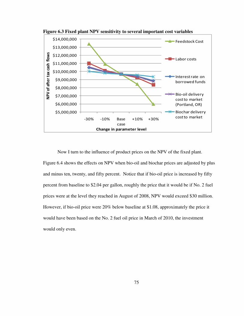
75

Figure 6.3 Fixed plant NPV sensitivity to several important cost variables

Now I turn to the influence of product prices on the NPV of the fixed plant.

Figure 6.4 shows the effects on NPV when bio-oil and biochar prices are adjusted by plus

and minus ten, twenty, and fifty percent. Notice that if bio-oil price is increased by fifty

percent from baseline to $2.04 per gallon, roughly the price that it would be if No. 2 fuel

prices were at the level they reached in August of 2008, NPV would exceed $30 million.

However, if bio-oil price were 20% below baseline at $1.08, approximately the price it

would have been based on the No. 2 fuel oil price in March of 2010, the investment

would only even.

$5,000,000

$6,000,000

$7,000,000

$8,000,000

$9,000,000

$10,000,000

$11,000,000

$12,000,000

$13,000,000

$14,000,000

-30% -10% Base

case

+10% +30%

NP

V o

f af

ter

tax

cash

flo

ws

Change in parameter level

Feedstock Cost

Labor costs

Interest rate on

borrowed funds

Bio-oil delivery

cost to market

(Portland, OR)

Biochar delivery

cost to market

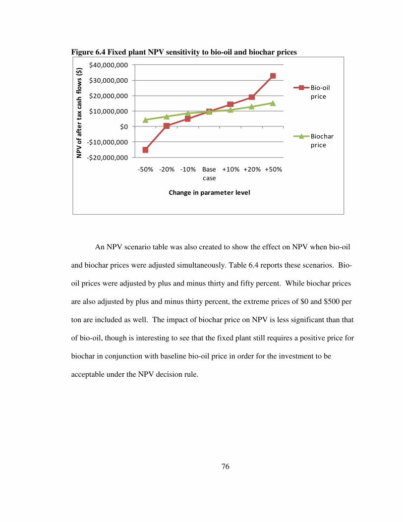
76

Figure 6.4 Fixed plant NPV sensitivity to bio-oil and biochar prices

An NPV scenario table was also created to show the effect on NPV when bio-oil

and biochar prices were adjusted simultaneously. Table 6.4 reports these scenarios. Bio-

oil prices were adjusted by plus and minus thirty and fifty percent. While biochar prices

are also adjusted by plus and minus thirty percent, the extreme prices of $0 and $500 per

ton are included as well. The impact of biochar price on NPV is less significant than that

of bio-oil, though is interesting to see that the fixed plant still requires a positive price for

biochar in conjunction with baseline bio-oil price in order for the investment to be

acceptable under the NPV decision rule.

-$20,000,000

-$10,000,000

$0

$10,000,000

$20,000,000

$30,000,000

$40,000,000

-50% -20% -10% Base

case

+10% +20% +50%

NP

V o

f af

ter

tax

cash

flo

ws

($)

Change in parameter level

Bio-oil

price

Biochar

price

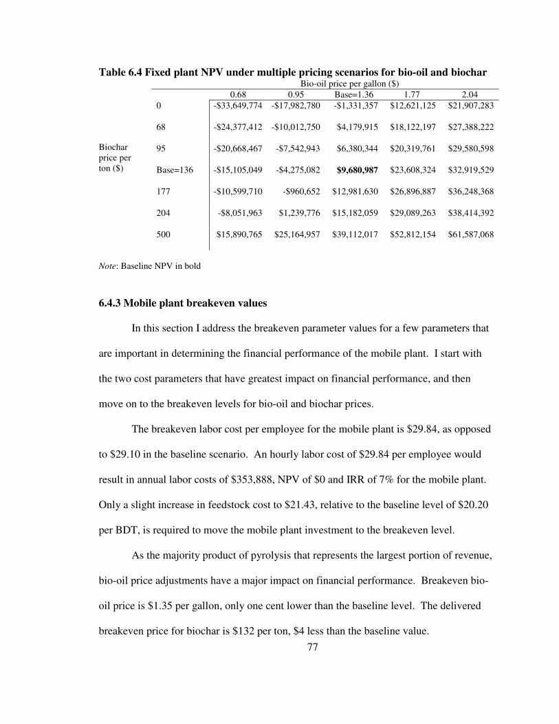
77

Table 6.4 Fixed plant NPV under multiple pricing scenarios for bio-oil and biochar Bio-oil price per gallon ($)

Biochar price per ton ($)

0.68 0.95 Base=1.36 1.77 2.04

0 -$33,649,774 -$17,982,780 -$1,331,357 $12,621,125 $21,907,283

68 -$24,377,412 -$10,012,750 $4,179,915 $18,122,197 $27,388,222

95 -$20,668,467 -$7,542,943 $6,380,344 $20,319,761 $29,580,598

Base=136 -$15,105,049 -$4,275,082 $9,680,987 $23,608,324 $32,919,529

177 -$10,599,710 -$960,652 $12,981,630 $26,896,887 $36,248,368

204 -$8,051,963 $1,239,776 $15,182,059 $29,089,263 $38,414,392

500 $15,890,765 $25,164,957 $39,112,017 $52,812,154 $61,587,068

Note: Baseline NPV in bold

6.4.3 Mobile plant breakeven values

In this section I address the breakeven parameter values for a few parameters that

are important in determining the financial performance of the mobile plant. I start with

the two cost parameters that have greatest impact on financial performance, and then

move on to the breakeven levels for bio-oil and biochar prices.

The breakeven labor cost per employee for the mobile plant is $29.84, as opposed

to $29.10 in the baseline scenario. An hourly labor cost of $29.84 per employee would

result in annual labor costs of $353,888, NPV of $0 and IRR of 7% for the mobile plant.

Only a slight increase in feedstock cost to $21.43, relative to the baseline level of $20.20

per BDT, is required to move the mobile plant investment to the breakeven level.

As the majority product of pyrolysis that represents the largest portion of revenue,

bio-oil price adjustments have a major impact on financial performance. Breakeven bio-

oil price is $1.35 per gallon, only one cent lower than the baseline level. The delivered

breakeven price for biochar is $132 per ton, $4 less than the baseline value.

78

6.4.4 Fixed plant breakeven values

The fixed plant has a higher NPV and IRR in the baseline scenario, meaning that

larger adjustments in parameter levels are required to bring NPV to $0 and determine

breakeven values. The fixed plant breakeven values for feedstock costs, labor costs, bio-

oil and biochar prices are now presented.

Feedstock cost is the most important operating cost parameter for the fixed plant,

as shown in figure 6.2. The breakeven feedstock cost is $80.69 per BDT, representing a

78 percent increase from the baseline value of $45.33 per BDT. The baseline scenario

assumed a two-phase feedstock haul with a 10 mile roundtrip in the first phase and a 90

mile roundtrip for the second phase. The breakeven cost could be generated if the first

phase was increased to a 38 mile roundtrip, the second phase was increased to a 231 mile

roundtrip, or some combination of the two. Labor costs are the second most important

cost variable mentioned above. However, due to economies of scale at the larger facility

labor costs have considerably less impact on financial performance than they do for the

mobile plant. The breakeven labor cost per employee for the fixed plant is $92.93 per

hour.

Bio-oil breakeven price for the fixed plant is $1.08 per gallon, a 21% reduction

from the baseline of $1.36 per gallon. The lower impact that biochar has on financial

performance means that its delivered price must be adjusted by a larger amount to reach

the breakeven level. The fixed plant has a breakeven biochar price of $16 per ton,

compared to the baseline price of $136 per ton, showing that even though financial

79

performance of the fixed plant is strong, the fixed plant investment is not profitable

unless it is able to sell both bio-oil and biochar.

80

Chapter 7

Conclusion

This study has shown the expected financial performance of two potential

pyrolysis plant configurations in southwest Oregon that could use forest biomass as

feedstock. The feasibility of a mobile 50 BDTPD mobile plant was compared with that

of a 200 BDTPD fixed-site plant using a discounted cash flow analysis model created in a

spreadsheet software package. Net present value (NPV), internal rate of return (IRR) and

payback period were calculated for each plant.

Baseline results showed that the mobile plant would generate an NPV of $35,748,

an IRR of 7.4% and a payback period of 9 years. With a discount rate of 7% in the

baseline scenario, the financial performance of the mobile plant is only marginally

acceptable. The fixed plant showed superior returns under each of the financial

performance measures, with NPV, IRR and payback period of $9.68 million, 20.9%, and

6 years, respectively.

Sensitivity analyses on cost and revenue parameters were conducted with respect

to several cost and revenue variables. This revealed that the two most important

operating cost parameters for both plants are labor costs and feedstock costs. However,

labor costs are much more important for the mobile plant, while feedstock costs are the

most important cost parameter for the fixed plant. This was not surprising, as labor costs

represent the largest share of operating costs for the mobile plant and feedstock costs are

the largest share of costs for the fixed plant. Economies of scale with respect to labor at

81

the fixed plant suggest that an increase in real labor costs would have less of an impact on

overall financial performance.

Finally, the delivered prices for bio-oil and biochar were varied for each plant to

determine the breakeven levels. Baseline prices were $1.36 per gallon of bio-oil and

$136 per ton of biochar for both plants. The mobile plant breakeven level was only 0.7%

lower at $1.35 per gallon and the fixed plant breakeven level was 21% lower at $1.08 per

gallon. Biochar breakeven prices were determined to be $132 per ton for the mobile

plant, a 3% decrease from the baseline, and $16 per ton for the fixed plant, an 88%

reduction from the baseline. This showed that even with fairly high returns in the

baseline scenario, the fixed plant would only be financially viable if it is able to earn

positive revenues from both bio-oil and biochar.

This study was conducted to aid stakeholders in understanding the determinants

of financial performance of fast pyrolysis plants using forest residues as feedstock. It is

necessary to keep in mind that the social benefits of the pyrolysis plants have not been

accounted for in this analysis, but they could be very important. Potential benefits

include increasing the viability of fuel treatments for ecosystem restoration and decreased

risk of catastrophic fire, especially in the wildland-urban interface (Stetler 2008;

O’Donnell 2009). Possible reductions in CO2, nitrous and sulfur oxides, and particulate

emissions, relative to fossil fuels, should also be considered by stakeholders. Reduced

dependency on foreign energy is an additional benefit that is important to policy makers

but has not been quantified in this analysis.

The analysis could be used as a starting point for determining the financial

feasibility of a potential project and it can be assumed that any available investment

82

incentives or preferential legislation would improve the investment outlook. Market

conditions for substitute products (fuel oil, coal, soil amendments) are very important to

financial performance and could either improve or decrease the attractiveness of the

investments compared to the scenarios presented in the results chapter.

It is wise to consider the results of this analysis while taking several caveats into

account as well. Many of the input data used in the financial model that analyzed the 50

and 200 BDTPD pyrolysis plants were obtained from ROI. However, ROI has not yet

manufactured a plant larger than 15 BDTPD. Therefore, there could be unforeseen

challenges and costs associated with scaling up the technology that were not captured by

this analysis.

While researchers and firms have been developing fast pyrolysis technology for

multiple decades, it is a relatively young industry and so far there is not a particular plant

configuration or reactor technology is obviously superior to others. Also, markets for

bio-oil and biochar are not well-developed. Due to the acidic and corrosive nature of bio-

oil, it is uncertain whether the 10% discount on a per MMBtu basis would induce

consumers to switch from No. 2 fuel oil to bio-oil. If bio-oil pricing was based on a

lower quality fuel such as No. 6 fuel oil, or ‘bunker fuel’, financial performance of the

investments would suffer significantly. This represents a risk that a potential investor

would need to consider. The risk of a much larger capital investment for the fixed plant

should also be taken into account. The larger capital investment required for the fixed

plant may justify the use of a higher, risk-adjusted discount rate.

Further research on GHG emissions from mobile and fixed site pyrolysis plants is

recommended, as well as the benefits associated with fossil fuel switching and carbon

83

sequestration in soils. The potential non-market benefits from implementing pyrolysis of

forest biomass on a broad scale, such as avoided deforestation and improved soils, are

also intriguing and important areas of additional research.

84

References ABRI, Advanced Biorefinery, Inc. (2010), available at: www.advbiorefineryinc.ca,

accessed 31 March 2010. Amonette, J. (2009), ‘An Introduction to Biochar: Concept, Processes, Properties, and

Applications’, Harvesting Clean Energy conference presentation, Billings, MT, 25 January 2009, available at: http://www.harvestcleanenergy.org/conference/HCE9/Post-conference/PPT/JimAmonette.pdf.

Anderson, N. (2010), ‘Up in smoke or in the black: Quantifying the productivity and

costs of forest biomass energy’, RMRS Lunch Seminar presentation, Missoula, MT, 26 February 2010.

Badger, P., Fransham, P. (2006), ‘Use of mobile fast pyrolysis plants to densify biomass

and reduce biomass handling costs—A preliminary assessment’, Biomass &

Bioenergy, 30(4): 321-325. Badger, P. (2006), ‘A new vision for value added forestry’, Maine Biomass and Biofuels

conference presentation. 20-22 Sep 2006. Badger, P. (2010), Renewable Oil International, LLC, personal communication, 24

January 2010. Badger, S. (2008), Renewable Oil International, LLC, personal communication, 30

October 2008. Badger, S. (2009a), Renewable Oil International, LLC, personal communication, 7

January 2009. Badger, S. (2009b), Renewable Oil International, LLC, personal communication, 20

March 2009. Badger, S. (2009c), Renewable Oil International, LLC, personal communication, 8 May

2009. Badger, S. (2009d), Renewable Oil International, LLC, personal communication, 14 July

2009. BLS, Bureau of Labor Statistics (2009a), available at:

http://data.bls.gov/PDQ/outside.jsp?survey=en, accessed 7 October 2009.

85

BLS, Bureau of Labor Statistics (2009b), available at: http://www.bls.gov/data/#employment, accessed 7 October 2009.

BLS, Bureau of Labor Statistics (2009c), CPI Inflation Calculator, available at:

http://stats.bls.gov/data/inflation_calculator.htm, accessed 7 October 2009. Boardman, A.E., Greenberg, D.H., Vining, A.R., and Weimer, D.L. (2006), Cost-Benefit

Analysis: Concepts and Practice, Pearson Prentice Hall, Upper Saddle River, NJ. Bouchard, T. (2009), Chief Operating Officer, Dynamotive Energy Systems Corporation,

Personal Communication, 26 March 2009. Bradley, C. (2009), ‘Montana Microbial Products 2nd Generation Ethanol’, Harvesting

Clean Energy conference presentation, Billings, MT, 27 January 2009, available at: http://www.harvestcleanenergy.org/conference/HCE9/Post-conference/PPT/CliffBradley.pdf

Bridgewater, A. (1999), ‘An introduction to fast pyrolysis of biomass for fuels and

chemicals’, in Bridgewater, A., Czernick, S., Diebold, J., Oasmaa, A., Peacocke, C., Piskorz, J., Radlein, D. (eds), Fast Pyrolysis of Biomass: A Handbook, Newbury, CPL Press, pp.1-13.

Bridgewater, A. (2002), in Bridgewater AV (ed), Fast Pyrolysis of Biomass: A

Handbook, Vol. 2, Newbury, CPL Press, pp.1-22. Bridgewater, A. (2004), ‘Biomass fast pyrolysis’, Thermal Science, 8(2): 21-49. Bridgewater, A. (2007), ‘IEA Bioenergy 27th Update’, Biomass and Bioenergy, 31(4):

VII-XVIII. Brown, R. (2009), ‘Biochar production technology’, in Lehmann, J. and Joseph, S. (eds),

Biochar for Environmental Management: Science and Technology, Earthscan, Sterling, VA, pp. 127-139

CAT, Caterpillar Performance Handbook (2007), Edition 37. pp. 20-11 (skid steer) and

20-28 (914G) Cattolica, R. (2009), ‘UCSD Biomass to Power Economic Feasibility Study’, UCSD

Sustainability Solutions Institute, UC San Diego. Caputo, A., Palumbo, M., Pelagagge, P., and Scacchia, F. (2005), ‘Economics of biomass

energy utilization in combustion and gasification plants: effects of logistic variables’, Biomass & Bioenergy, 28(1): 35-51.

86

Carter, K. (2009), Sales Associate, Peterson Machinery, Eugene, Oregon, Personal

communication, 9 October 2009. Cheng, C-Hsin, Lehmann, J., Thies, J. E., and Burton, S. D. (2008) ‘Stability of black

carbon in soils across a climatic gradient’, Journal of Geophysical Research, 113:G02027.

Chung, W. (2009), Personal Communication, July 2009. ClearSky Climate Solutions (2010), available at:

http://www.clearskyclimatesolutions.com/work/projects/index.html, accessed 29 March 2010.

Cloughesy, M. (2009), ‘Biomass Energy and Biofuels from Oregon’s Forests’,

Presentation at Roseburg Public Library, 19 Aug 2009. Cole Hill Associates (2004), ‘Bio-Oil Commercialization Plan – Prepared for the NH

Office of Planning and Energy’, July 2004. Curtis, N. (2009), Willamette National Forest, Personal communication, 16 April 2009. Dayanda, D., Irons, R., Harrison, S., Herbohn, J., and Rowland, P. (2002), Capital

Budgeting: Financial Appraisal of Investment Projects, Cambridge University Press, Cambridge.

Dirksen, J. (2009). Dirksen & Sons, Roseburg, OR, Personal Communication, 30 July

2009. Dykstra, D. (2009). U.S. Forest Service PNW Research Station, Personal

Communication. 22 July 2009. Dynamotive (2009). Dynamotive Energy Systems Corporation, Canadian BioOil Plant:

Summary (USD), available at www.dynamotive.com, accessed 24 April 2009 Dynamotive (2010), available at: http://www.dynamotive.com/about/corporate_history/

accessed 31 March, 2010. EIA, Energy Information Administration (2007), Annual Energy Outlook 2007: With

Projections to 2030, DOE/EIA-0383(2007). EIA, Energy Information Administration (2009a), available at:

http://tonto.eia.doe.gov/dnav/pet/PET_PRI_PROP_DCU_R50_A.htm, accessed 10 November 2009.

87

EIA, Energy Information Administration (2009b), available at http://www.eia.doe.gov/cneaf/electricity/epm/table5_6_b.html#_ftn1, accessed 10 November 2009.

EIA, Energy Information Administration (2009c), available at http://www.eia.doe.gov/basics/conversion_basics.html, accessed 12 November 2009.

EIA, Energy Information Administration (2009d), available at http://tonto.eia.doe.gov/dnav/pet/pet_pri_dist_dcu_nus_m.htm, accessed 20 November 2009.

EIA, Energy Information Administration (2010a), available at:

http://www.eia.doe.gov/cneaf/alternate/page/renew_energy_consump/figure1.html, accessed 10 April 2010.

EIA, Energy Information Administration (2010b), available at:

http://tonto.eia.doe.gov/state/state_energy_profiles.cfm?sid=OR, accessed 10 April 2010.

Ensyn (2010), available at: www.ensyn.com, accessed 31 March, 2010 Ensyn (2001), The Conversion of Wood and Other Biomass to Bio-oil. 13p. Farag, I., LaClair, C., Barrett, C. (2002), Final Report: Technical, Environmental and

Economic Feasibility of Bio-Oil in New Hampshire’s North Country. Durham, NH: University of New Hampshire.

Fight, R., Hartsough, B., Noordijk, P. (2006), Users Guide for FRCS: Fuel Reduction

Cost Simulator Software, USDA Forest Service, General Technical Report PNW-GTR-668.

Fournier, Jim (2009), ‘Low Temperature Pyrolysis for Biochar Systems’, Harvesting

Clean Energy conference presentation, Billings, MT, 25 January 2009. Gaunt, J., Lehmann, J. (2008), ‘Energy balance and emissions associated with biochar

sequestration and pyrolysis bioenergy production’, Environmental Science and

Technology, 42(11): 4152-4158. Glaser, B. Haumaier, L., Guggenberger, G., Zech, W. (2001), ‘The Terra Preta

phenomenon: A model for sustainable agriculture’, Naturwissenschaften, 88(2001): 37-41.

88

Goodfellow, R. (2008), ‘Pyrolysis: Bio-Energy, Bio-Chemicals, and Renewable Transport Fuel’, Advanced Biofuels Workshop conference presentation, Minneapolis, MN, 29 September 2008

Han, H., Lee, H., Johnson, L. (2004), ‘Economic feasibility of an integrated harvesting

system for small diameter trees in southwest Idaho’, Forest Products Journal, 54(2): 21-27.

Herzog, Mike (2009), Sales Associate, Western States CAT. Personal communication. July 13, 2009.

Hill, J., Nelson, E., Tilman, D., Polasky, S., and Tiffany, D. (2006), ‘Environmental,

economic, and energetic costs and benefits of biodiesel and ethanol biofuels’, Proceedings of the National Academy of Sciences, 103(30): 11206-11210.

IBI, International Biochar Initiative (2010), available at: http://www.biochar-

international.org/biochar, accessed 22 Feb 2010. IPCC, Intergovernmental Panel on Climate Change (2000), Land Use, Land Use Change,

and Forestry. Cambridge University Press, Cambridge. IPCC (2007), Climate Change 2007: Synthesis Report, Summary for Policy Makers,

Intergovernmental Panel on Climate Change. Geneva, Switzerland. IRS, Internal Revenue Service, (2009), Instructions for form 1120, U.S. Corporation

Income Tax Return, Schedule J. Brinker, R., Kinard, J., Rummer, B. and Lanford, B. (2002), ‘Machine rates for selected

harvesting machines’, Alabama Agricultural Experiment Station. Auburn University.

Page-Dumroese, D. (2010), USDA Forest Service Rocky Mountain Research Station, ‘In-woods portable pyrolysis of forest biomass and the application of the byproduct bio-char in a field trial’, 12 January 2010.

Joseph, S. and Watts, P. (2009), ‘Large-scale Bioenergy and biochar’, Case Study I in

Chapter 9, Lehmann, J. and Joseph, S. (eds), Biochar for Environmental Management: Science and Technology. Earthscan, Sterling, VA.

Kerns, Brian (2009), ‘University of Montana Bio-Energy Project’, Harvesting Clean

Energy conference presentation, Billings, MT, 27 January 2009, available at: http://www.harvestcleanenergy.org/conference/HCE9/Post-conference/PPT/BrianKerns.pdf

89

Laird, D., Brown, R., Amonette, J., Lehmann, J. (2009), Review of the pyrolysis platform for coproducing bio-oil and biochar’ Biofuels, Bioprod., Bioref., 3:547-562.

Lal, R. (2004), ‘Soil Carbon Sequestration Impacts on Global Climate Change and Food

Security’, Science, 304: 1623-1627. Lawrence, Joe (2009), County Commissioner, Douglas County, Oregon. Presentation at

Roseburg Public Library, 19 Aug 2009. Lehmann, J. (2007), ‘A handful of carbon’, Nature, 447: 143-144. Lehmann, J., Gaunt, J., Rondon, M. (2006), ‘Bio-char Sequestration in Terrestrial

Ecosystems – A Review’, Mitigation and Adaptation Strategies for Global Change, 11:403-427.

Lehmann, J. and Joseph, S. (2009), ‘Biochar for Environmental Management: An

Introduction’, in Lehmann, J. and Joseph, S. (eds.), Biochar for Environmental

Management: Science and Technology, Earthscan, Sterling, VA, pp.1-9. Lewis, Trevor (2009), Business Relationship Manager, Wells Fargo Bank N.A.,

Missoula, MT, Personal Communication, 21 July 2009. Loeffler, D. (2004), ‘An Analysis of Small Diameter Forest Biomass Availability and

Removal Costs in Ravalli County, Montana’, Master’s thesis, University of Montana.

Loeffler, D., Calkin, D., Silverstein, R. (2006), ‘Estimating volumes and costs of forest

biomass in Western Montana using forest inventory and geospatial data’, Forest Products Journal, 56(6): 31-37.

Lynd, L., Cushman, J., Nichols, R., and Wyman, C. (1991), ‘Fuel ethanol from cellulosic

biomass’, Science, New Series, 21(4999): 1318-1323. Lynd, L., Elander, R., Wyman, C. (1996), ‘Likely features and costs of mature biomass

ethanol technology’, Applied Biochemistry and Biotechnology, 57/58(1996): 741-761.

Matthews, J. (2008), ‘Carbon-negative biofuels’, Energy Policy, 36(2008): 940-945. McGill, Josh (2009a), Renewable Oil International, LLC, personal communication, 17

July 2009. McGill, Josh (2009b), Renewable Oil International, LLC, personal communication, 6

Nov 2009.

90

McKendry, P. (2002a), ‘Energy production from biomass (part 1): Overview of biomass’, Bioresource Technology, 83(2002): 37-46.

McKendry, P. (2002b), ‘Energy production from biomass (part 2): Conversion

technologies’, Bioresource Technology, 83(2002): 47-54. Miles, T. ‘The Economics of Biochar Production.’ PNW Biochar Group Meeting,

Richland, WA, 21-22 May 2009. Mohan, D., Pittman, Jr., C., Steele, P. (2006) ‘Pyrolysis of Wood/Biomass for Bio-oil: A

Critical Review’, Energy and Fuels, 20(3): 848-889. Nelson, Steve (2009), Contracting Officer, Umpqua National Forest, personal

communication, 10 July 2009. Oasmaa, A., Czernick, S. (1999), ‘Fuel oil quality of biomass pyrolysis oils—state of the

art for end users’, Energy & Fuels, 13(4): 914-921 ODEQ, Oregon Department of Environmental Quality (2009), ‘2008 Oregon Air Quality

Data Summaries’, Portland, OR, 111p. O’Donnell, D. (2009), ‘Social Values for Attributes at Risk from Wildfire in Northwest

Montana’, Master’s thesis, University of Montana. OFRI, Oregon Forest Resources Institute (2007), ‘Woody Biomass Energy: A Renewable

Resource to Help Meet Oregon’s Energy Needs’, Portland, OR, 13p. OFRI, Oregon Forest Resources Institute (2002), ‘Fire in Oregon’s Forests: Assessing

the Risks, Effects, and Treatment Options’, Portland, OR, 16p. Perlack, R., Wright, L., Turhollow, A., Graham, R., Stokes, B., and Erbach, D. (2005),

‘Biomass as feedstock for a bioenergy and bioproducts industry: The technical

feasibility of a billion-ton annual supply’. U.S. Department of Agriculture and U.S. Department of Energy, Washington, D.C.,

Pine, J. (2009), Biomass Coordinator, Oregon Department of Foresty, personal

communication, October 2009. Radlein D. and Bouchard, T. (2009), ‘A preliminary look at the economics of a new

biomass conversion process by DynaMotive’, accessed at www.dynamotive.com on April 24, 2009

Rawlings, C., Rummer, B., Seeley, C., Thomas, C., Morrison, D., Han, H., Cheff, L.,

Atkins, D., Graham, D., and Windell, K. (2004), ‘A Study of How to Decrease the

91

Costs of Collecting, Processing and Transporting Slash’, Montana Community Development Corporation, Missoula, MT.

RFA, Renewable Fuels Association (2010), available at:

http://www.ethanolrfa.org/industry/statistics/, accessed 25 March 2010. Richardson, J., Herbst, B., Outlaw, J., Gill II, R. (2007), ‘Including risk in economic

feasibility analyses: The case of ethanol production in Texas’, Journal of

Agribusiness, 25,2(fall 2007): 115-132. Ringer, M., Putsche, V., and Scahill, J. (2006), ‘Large-Scale Pyrolysis Oil Production: A

Technology Assessment and Economic Analysis’, Technical Report NREL/TP-510-37779. National Renewable Energy Laboratory, Golden, CO.

Rummer, B., Prestemon, J., May, D., Miles, P., Vissage, J., McRoberts, R., Liknes, G.,

Sheppard, W., Ferguson, D., Elliot, W., Miller, S., Reutebuch, S., Barbour, J., Fried, J., Stokes, B., Bilek, E., and Skog, K. (2005), ‘A strategic assessment of forest biomass and fuel reduction treatments in Western states’, USDA Forest Service, Rocky Mountain Research Station, General Technical Report RMRS-GTR-149.

Runge, C. and Senauer, B. (2007), ‘How biofuels could starve the poor’, Foreign Affairs,

86(3): 41-53. Searchinger, T., Heimlich, R., Houghton, R.A., Dong, F., Elobeid, A., Fabiosa, J.,

Tokgoz, S., Hayes, D., Yu, T. (2008), ‘Use of US croplands for biofuels increases greenhouse gases through emissions from land-use change’, Science, 319: 1238-1240.

Silverstein, R.P., Loeffler, D.R., Jones, J.G., Calkin, D.E., Zuuring, H., Twer, M. (2006),

‘Biomass Utilization Modeling on the Bitterroot National Forest’, USDA Forest Service Proceedings, RMRS-P-41.

Soltes, E. and Elder, T. (1981), Pyrolysis, In Organic Chemicals from Biomass, Goldstein

IS. (ed.) CRC Press, Florida. pp. 63-100. Sombroek, W., Ruivo, M.L., Fearnside, P.M., Glaser, B., and Lehmann, J. (2003),

‘Amazonian Dark Earths as stores and sinks’, in J. Lehmann, D.C. Kern, B. Glaser and W.I. Woods (eds.) Amazonian Dark Earths: Origin, Properties,

Management, (pp 125-139) Dordrecht, Kluwer Academic Publishers. Spelter, H. (2009), ‘Roseburg Repeat’, Timber Processing, July/Aug, pp. 18-20.

92

Stetler, K. (2008), ‘Capitalization of Environmental Amenities and Wildfire in Private

Home Values of the Wildland-Urban Interface of Northwest Montana, USA’, Master’s thesis, University of Montana.

van Vilet, O., Faaij, A., and Turkenburg, W. (2009), ‘Fischer-Tropsch diesel production

in a well-to-wheel perspective: A carbon, energy flow and cost analysis’, Energy

Conversion and Management, 50(2009): 855-876. Wang, M., Wu, M., and Huo, H. (2007), ‘Life cycle energy and greenhouse gas emission

impacts of different corn ethanol plant types’, Environmental Research Letters, 2(2007):1-13.

Warnock, D., Lehmann, J., Kuyper, T., and Rillig, M. (2007), ‘Mycorrhizal responses to

biochar in soil – concepts and mechanisms’, Plant Soil, 300:9-20. Whitaker, Gene (2009), President, Whit-Log Trailers, Personal communication, 23

November 2009. Wiedenbeck, J. and Blackwell, K. (2003), ‘Hardwood Sawmill Downtime Costs’,

Southern Lumberman, May, pp. 27-30. Wiltsee, G. (2000), ‘Lessons Learned from Existing Biomass Power Plants’, NREL/SR-

57026946, National Renewable Energy Laboratory, Golden, CO. Winsley, P. (2007), ‘Biochar and bioenergy production for climate change mitigation’,

New Zealand Science Review, 64(1): 5-10 Wood, K. (2009), President, Gordon Wood Insurance, personal communication, 9

October. Yaman, S. (2004), ‘Pyrolysis of biomass to produce fuels and chemical feedstocks’,

Energy Conversion and Management, 45(2004): 651-671.

93

Appendix A

Additional sensitivity analyses

A.1 Mobile plant sensitivity analyses (baseline values in bold) Initial capital investment Parameter level $2,421,300 $3,113,100 $3,459,000 $3,804,900 $4,496,700

NPV $736,995 $283,188 $35,748 -$231,724 -$815,462

Hourly labor cost per employee Parameter level $20 $26 $29.10 $32 $37.83

NPV $414,986 $171,657 $35,748 -$109,076 -$429,916

Discount rate Parameter level

4.0% 5.5% 7.0% 8.5% 10.0% 11.5% 13.0%

NPV $343,229 $179,366 $35,748 -$90,477 -$201,717 -$300,015 -$387,106

Scheduled hours per day Parameter level 8 9 10 11 12

NPV -$1,047,754 -$746,594 -$463,086 -$200,855 $35,748

Moves per year Parameter level 1 2 4 7 10

NPV $54,135 $35,748 -$1,430 -$59,297 -$118,696

Energy cost (propane, $/gallon) Parameter level $1.60 $2.05 $2.28 $2.51 $2.96

NPV $117,230 $63,133 $35,748 $8,237 -$49,000

Bio-oil yield (% of feedstock weight, assuming 10% moisture content in feedstock) Parameter level

55.0% 56.0% 57.0% 58.0% 59.0% 60.00%

NPV -$46,726 -$4,750 $35,748 $75,745 $115,139 $153,865

94

Energy content of bio-oil (MMBtu/gallon) Parameter level 0.0750 0.0775 0.0800 0.0825 0.0850

NPV -$292,301 -$122,386 $35,748 $183,452 $327,614

Percentage of initial capital investment borrowed Parameter level 42% 54% 60% 66% 78%

NPV -$6,886 $23,030 $35,748 $46,148 $60,477

Feedstock average roundtrip distance (miles) Parameter level 7 9 10 11 13

NPV $142,334 $71,776 $35,748 -$662 -$76,301

Pyrolysis system generator efficiency Parameter level 21.0% 27.0% 30.0% 33.0% 39.0%

NPV -$244,003 -$33,173 $35,748 $90,660 $172,667

A.2 Fixed plant sensitivity analyses (baseline values in bold)

Initial capital investment Parameter level $16,979,200 $21,830,400 $24,256,000 $26,681,600 $31,532,800

NPV $17,460,190 $12,274,055 $9,680,987 $7,087,919 $1,901,783

Hourly labor cost per employee Parameter level $20 $26 $29.10 $32 $37.83

NPV $11,005,119 $10,122,364 $9,680,987 $9,239,610 $8,356,855

Discount rate Parameter level

4.0% 5.5% 7.0% 8.5% 10.0% 11.5% 13.0%

NPV $13,591,424 $11,510,971 $9,680,987 $8,066,592 $6,638,282 $5,371,028 $4,243,539

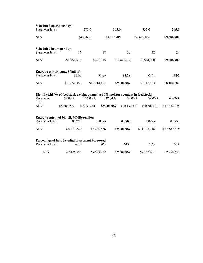
95

Scheduled operating days Parameter level 275.0 305.0 335.0 365.0

NPV $488,686 $3,552,786 $6,616,886 $9,680,987

Scheduled hours per day Parameter level 16 18 20 22 24

NPV -$2,757,579 $361,015 $3,467,672 $6,574,330 $9,680,987

Energy cost (propane, $/gallon) Parameter level $1.60 $2.05 $2.28 $2.51 $2.96

NPV $11,257,386 $10,214,181 $9,680,987 $9,147,793 $8,104,587

Bio-oil yield (% of feedstock weight, assuming 10% moisture content in feedstock) Parameter level

55.00% 56.00% 57.00% 58.00% 59.00% 60.00%

NPV $8,780,294 $9,230,641 $9,680,987 $10,131,333 $10,581,679 $11,032,025

Energy content of bio-oil, MMBtu/gallon Parameter level 0.0750 0.0775 0.0800 0.0825 0.0850

NPV $6,772,728 $8,226,858 $9,680,987 $11,135,116 $12,589,245

Percentage of initial capital investment borrowed Parameter level 42% 54% 60% 66% 78%

NPV $9,425,343 $9,595,772 $9,680,987 $9,766,201 $9,936,630

96

Appendix B

Cost parameter tables

Table B.1 Mobile plant delivered feedstock costs Parameter Level

Biomass stumpage ($/ton at 30% moisture content) 0.09a

Haul cost ($/hr) 110b

Speed (mph) 10c

Average roundtrip haul distance (miles) 10c

Truck capacity (tons) 12.5c

Annual delivered feedstock (tons @ 30% moisture content)

10,182d

Annual delivered feedstock (BDT equivalent) 7,128d

Annual feedstock haul costs ($) 89,604d

Chipping cost ($/BDT) 7.50e

Annual chipping cost 53,460e

Annual prepared feedstock cost 143,978e

Sources: a) Curtis (2009) b) Chung 2009 c) author’s estimate d) Dykstra (2009) e) spreadsheet calculation

Table B.2 Mobile plant feedstock loading costs (Caterpillar 262 Skid Steer) Parameter Level

Bucket size (cubic yards) 1a

Buckets per ton of feedstock 4b

Cycles per hour 40a

Feedstock density (pounds/yard3) 500c

Fuel consumption (gal/hr) 2d

Operating hours per day 3.1b

Annual fuel cost ($) 5,437b

Annual tire replacement cost ($) 2,444a

Annual maintenance cost ($) 2,445a

Total annual loader costs ($) 10,326b

Sources: a) Herzog (2009). b) spreadsheet calculation. c) McGill (2009a) d) CAT (2007).

97

Table B.3 Mobile plant energy consumption and costs Parameter Level

Thermal energy cost (propane, $/gal) 2.28a

Thermal energy required (MMBtu/hr) 3.22b

Percentage of thermal energy purchased for mobile plant 25b

Propane energy content (MMBtu/gal) 0.091a

Purchased thermal energy (propane, gal/hr) 8.81c

Annual cost for purchased energy ($) 68,109c

Sources: a) EIA (2009c). b) Badger (2009a) c) spreadsheet calculation

Table B.4 Mobile plant bio-oil delivery costs Parameter Level

Gallons sold per year 780,642a

Transport cost in cents/gallon .1122b

Annual fuel delivery cost $87,588a

Sources: a) spreadsheet calculation. b) Dirksen (2009)

Table B.5 Mobile plant biochar delivery costs Parameter Level

Trucking cost ($/hr) 75a

Truck capacity (tons) 27.5a

Round trip biochar haul to market (hrs) 5b

Cost of one round trip delivery ($) 375a

Annual tons of biochar to market 2138c

Annual biochar delivery cost ($) 29,158c

Sources: a) Whitaker (2009). b) author’s estimate. c) spreadsheet calculation

98

Table B.6 Fixed plant initial capital investment Parameter Level

Pyrolysis system ($) 15,000,000a

Land ($) 2,000,000b

Building ($) 4,000,000a

Outside improvements ($) 2,000,000a

Loader cost (2 loaders at $128,000 each) ($) 256,000c

Non-pyrolysis building contents ($) 1,000,000a

Total capital investment ($) 24,256,000c

Sources: a) author’s estimate. b) Nelson (2009). c) Carter (2009)

Table B.7 Fixed plant investment and financing costs Parameter Level

Initial Capital Investment ($) 24,256,000a

Down Payment ($) 9,702,400a

Interest Rate on Borrowed Funds (%) 9b

Term of Loan (years) 7b

Annual Loan Payment ($) 2,891,662a Sources: a) spreadsheet calculation. b) Badger (2009a); Lewis (2009). Table B.8 Fixed plant labor costs Parameter Level

Average hourly wage including fringe ($) 29.10a

Annual hours paid per employee 2080b

Average # of employees per operating hour 4.6c

Number of employees 17.5c

Annual labor cost ($) 1,059,240c

Sources: a) BLS (2009a) b) 40hours per week, 52 weeks per year. c) based on Farag et al. (2002). See Appendix C. d) spreadsheet calculation

99

Table B.9 Fixed plant delivered feedstock costs Parameter Level

Biomass stumpage ($/ton at 30% moisture content) 0.09a

In-woods haul cost to concentration yard ($/hr) 110b

Speed (mph) 10c

Average roundtrip haul distance (miles) 10c

Truck capacity (tons) 12.5c

Haul cost from concentration yard to fixed plant ($/hr) 110b

Speed (mph) 25c

Average roundtrip haul distance (miles) 90c

Concentration yard handling cost ($/BDT) 2.5c

Annual delivered feedstock (tons @ 30% moisture content) 93,857d

Annual delivered feedstock (BDT equivalent) 65,700d

Annual feedstock haul costs ($) 2,476,890d

Chipping cost ($/BDT) 7.50e

Annual chipping cost 492,750d

Annual delivered feedstock cost 2,978,087d

Sources: a) Curtis (2009) b) Chung (2009) c) author’s estimate d) spreadsheet calculation e) Dykstra (2009)

Table B.10 Fixed plant feedstock loading costs (Caterpillar 914G Wheel Loader) Parameter Level

Bucket size (cubic yards) 4a

Buckets per ton of feedstock 1b

Cycles per hour 40a

Fuel consumption (gal/hr) 2.25c

Operating hours per day 6.3d

Annual fuel cost ($) 13,885b

Annual tire replacement cost ($) 4,067a

Annual maintenance cost ($) 5,390a

Total annual loader costs ($) 23,342d

Sources: a) Carter (2009). b) spreadsheet calculation. c) CAT (2007). d) spreadsheet calculation.

100

Table B.11 Fixed plant energy consumption and costs Parameter Level

Thermal energy cost (propane, $/gal) 2.28a

Thermal process energy required (MMBtu/hr) 25.78b

Thermal energy purchased (%) 25b

Propane energy content (MMBtu/gal) 0.091c

Purchased thermal energy consumption for fixed plant (propane, gal/hr) 70.57d

Electrical energy cost ($/kWh) 0.0474e

Electrical energy required (MMBtu/hr) 2.99b

Energy content of electricity (MMBtu/kWh) 0.003412c

Electrical energy purchased for fixed plant (%) 100f

Annual thermal and electrical energy purchased ($) 1,595,941d

Sources: a) EIA 2009a. b) Badger (2009a). c) EIA (2009c). d) spreadsheet calculation. e) EIA (2009. f) McGill (2009b)

Table B.12 Fixed plant bio-oil delivery costs Transport cost parameter Level

Annual bio-oil sales (gal) 8,322,000a

Transport cost ($/gal) .0872b

Annual fuel delivery cost ($) 725,678a

Sources: a) spreadsheet calculation. b) Dirksen (2009)

Table B.13 Fixed plant biochar delivery costs Parameter Level

Trucking cost ($/hr) 75a

Truck capacity (tons) 27.5a

Round trip biochar haul to market (hrs) 5b

Cost of one round trip delivery ($) 375c

Number of truckloads/year 717c

Annual biochar delivery cost ($) 268,773c

Sources: a) Whitaker (2009). b) author’s estimate. c) spreadsheet calculation.

101

Appendix C

Fixed plant wages and benefits

The 2002 Farag et al. study assumed 9 employees are required for a facility

processing 100 metric tons of wood chips per day at 45% moisture content, and 12 and

15 employees for a 200 and 400 wet metric ton/day plants, respectively. I converted 200

wet metric tons per day to 121.2 BDTPD, and 400 wet metric tons per day to 242.4

BDTPD. To convert metric tons to US tons, I multiplied by the conversion factor 1.102,

and to convert from 45% moisture content to BDT (0% moisture content), I multiplied

that result by 1-moisture content, or 0.55. Equation: (200*1.102) * (1-0.45) = 121.2.

This means that as the plant increased in size from 121.2 BDTPD to 242.4

BDTPD, one additional employee was added for every additional 40.4 BDTPD. As I am

evaluating a 200 BDTPD plant, I added two employees to the 12 required for the 121.2

BDTPD plant and assumed 14 employees are required for the 200 BDTPD plant. Farag

et al. also assumed an additional 4 “non-production employees” with a total wage and

benefit bill (including 30% overhead) of $176,786 for the 400 wet metric ton plant. I

reduced that figure to 3.5 employees for a 200 BDTPD plant36, subtracted the overhead

rate, and converted from 2002 to 2008 dollars using the BLS CPI Inflation Calculator

(BLS 2009c). I then added the 35% fringe rate used in this study and added that to the

total wage and benefit bill including fringe. The total wage and benefit bill was then

converted to an average hourly labor cost of $30.51 per employee for the 17.5 full-time

36 According to Farag et al. (2002), 2 non-production employees are required for a 200 wet metric ton plant (equivalent to 121.2 BDTPD) and 4 are required for a 400 wet metric ton plant (equivalent to 242.4 BDTPD). Therefore, I assume 3.5 non-production employees are required for a 200 BDTPD plant.

102

equivalent employees at the 200 BDTPD plant. As this hourly rate was fairly close to the

rate of $29.10 used for the mobile plant analysis and based on wages in Douglas County,

Oregon, I elected to use the $29.10 rate as a baseline wage and benefit rate for both the

mobile and fixed plants.

103

Appendix D

U.S. Corporation Income Taxes

Table D.1 Federal tax rate schedule for 2008

Source: IRS (2009)

If taxable income is:

Over -- But not over -- Tax is -- of the amount over --

$0 $50,000 15% $0

$50,000 $75,000 $7,500 + 25% $50,000

$75,000 $100,000 $13,750 + 34% $75,000

$100,000 $335,000 $22,250 + 39% $100,000

$335,000 $10,000,000 $133,900 + 34% $335,000

$10,000,000 $15,000,000 $3,400,000 + 35% $10,000,000

$15,000,000 $18,333,333 $5,150,000 + 38% $15,000,000

$18,333,333 --------------- 35% $0

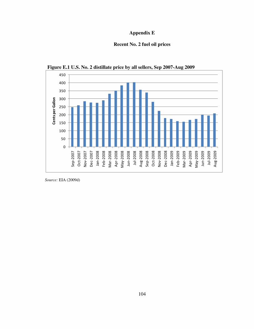
104

Appendix E

Recent No. 2 fuel oil prices Figure E.1 U.S. No. 2 distillate price by all sellers, Sep 2007-Aug 2009

Source: EIA (2009d)

0

50

100

150

200

250

300

350

400

450S

ep

-20

07

Oc

t-2

00

7

No

v-2

00

7

De

c-2

00

7

Jan

-20

08

Fe

b-2

00

8

Ma

r-2

00

8

Ap

r-2

00

8

May

-20

08

Jun

-20

08

Jul-

20

08

Au

g-2

00

8

Se

p-2

00

8

Oc

t-2

00

8

No

v-2

00

8

De

c-2

00

8

Jan

-20

09

Fe

b-2

00

9

Ma

r-2

00

9

Ap

r-2

00

9

May

-20

09

Jun

-20

09

Jul-

20

09

Au

g-2

00

9

Ce

nts

pe

r G

allo

n