2002 Special Issue

Image denoising using self-organizing map-based nonlinear independent

component analysis

Michel Haritopoulos*, Hujun Yin, Nigel M. Allinson

Department of Electrical Engineering and Electronics, UMIST, P.O. Box 88, Manchester M60 1QD, UK

Abstract

This paper proposes the use of self-organizing maps (SOMs) to the blind source separation (BSS) problem for nonlinearly mixed signals

corrupted with multiplicative noise. After an overview of some signal denoising approaches, we introduce the generic independent

component analysis (ICA) framework, followed by a survey of existing neural solutions on ICA and nonlinear ICA (NLICA). We then detail

a BSS method based on SOMs and intended for image denoising applications. Considering that the pixel intensities of raw images represent a

useful signal corrupted with noise, we show that an NLICA-based approach can provide a satisfactory solution to the nonlinear BSS

(NLBSS) problem. Furthermore, a comparison between the standard SOM and a modified version, more suitable for dealing with

multiplicative noise, is made. Separation results obtained from test and real images demonstrate the feasibility of our approach. q 2002

Elsevier Science Ltd. All rights reserved.

Keywords: Self-organizing maps; Independent component analysis; Nonlinear; Image denoising; Multiplicative noise

1. Introduction

One of the increasingly important tools in signal

processing is independent component analysis (ICA;

Comon, 1994). This was initially proposed to provide a

solution to the blind source separation (BSS) problem

(Herault, Jutten, & Ans, 1985), namely how to recover a set

of unobserved sources mixed in an unknown manner from a

set of observations. Since then, numerous algorithms based

on the ICA concept have been employed successfully in

various fields of multivariate data processing, from

biomedical signal applications and communications to

financial data modelling and text retrieval.

While linear mixtures of unknown sources have been

examined thoroughly in the literature, the case of nonlinear

ones remains an active field of research. This is due to the

reduced representation of real-world datasets by the

standard ICA formulation, which implies linear mixings

of independent source signals. A common assumption of

linear ICA-based methods is the absence of noise and that

the number of mixtures must, at least, equal the number of

sources.

Existing nonlinear ICA (NLICA) methods can be

classified into two categories (Lee, 1999). The first

models the nonlinear mixing as a linear process followed

by a nonlinear transfer channel. These methods are of

limited flexibility as they are often parametrized. On the

other hand, the second category employs parameter-free

methods, which are more useful in representing more

generic nonlinearities. A common neural technique in

this second category is the well known self-organizing

map (SOM), mainly used for the modelling and

extraction of underlying nonlinear data structures.

SOMs (Kohonen, 1997) are neural network-based tech-

niques using unsupervised learning and can provide

useful data representations, such as clusters, prototypes

or feature maps concerning the prototype (input) space.

Early work on the application of SOMs to the NLICA

problem has been done by Pajunen, Hyvarinen, and

Karhunen (1996) and Herrmann and Yang (1996).

Further work on NLICA has shown that there always

exists at least one solution that is highly nonunique.

However, additional constraints (e.g. the mixing function

must be a conformal mapping from R2 to R2 and

independent components must have bounded support

densities) are needed to guarantee uniqueness (Hyvarinen

& Pajunen, 1999).

The use of SOM-based separating structures can be

justified as SOMs perform a nonlinear mapping from an

input space to an output one usually represented as a low

dimensional lattice. Using some suitable interpolation

method (topological or geometrical), the map can be made

continuous to provide estimates of the unknown signals.

0893-6080/02/$ - see front matter q 2002 Elsevier Science Ltd. All rights reserved.

PII: S0 89 3 -6 08 0 (0 2) 00 0 81 -3

Neural Networks 15 (2002) 1085–1098

www.elsevier.com/locate/neunet

* Corresponding author. Tel.: þ44-161-200-4804; fax: þ44-161-200-

4784.

E-mail address: michelh@swift.ee.umist.ac.uk (M. Haritopoulos).

However, there are difficulties associated with the nonlinear

BSS (NLBSS) problem, such as its intrinsic indeterminacy

and the unknown distribution of sources as well as the

mixing conditions (which depend on the strength of the

unknown nonlinear function involved in the mixing

process), and the presence of noise (correlated or not). All

these make it difficult for a complete analytical study of

SOM behaviour when applied in this context.

The purpose of this paper is to show that an extended

SOM-based technique can perform NLICA for the denois-

ing of images. The advantages as well as the drawbacks of

this technique, associated mainly with its high compu-

tational cost, will be discussed. After an overview of some

signal denoising methods, followed by an introduction to

the generic ICA problem and a brief presentation of some

neural methods applied to the NLICA case, we will focus on

the SOM’s inherent nonlinear properties which make the

NLBSS problem tractable. Then, we detail an image

denoising scheme using SOMs. A comparative study

between a modified SOM algorithm (Der, Balzuweit, &

Herrmann, 1996), the original one and other nonlinear

denoising techniques such as kernel principal component

analysis (KPCA) and wavelet decomposition in the presence

of multiplicative noise, will be validated by simulations and

some real images.

2. Other signal denoising approaches

Image noise removal is traditionally achieved by linear

processing techniques such as Wiener, low-, high- or band-

pass filtering (Gonzalez & Woods, 2002). They can smooth

(low-pass filters), enhance high spatial frequency charac-

teristics (high-pass filters) or reduce specific noises (band-

pass filters), while Wiener filtering is optimal in the least

MSE sense. Their popularity is due to their mathematical

simplicity and efficiency in the presence of additive

Gaussian noise, but they tend to blur edges and do not

remove heavy tailed (salt and pepper type noise, for

example) and signal dependent noise. A classical nonlinear

alternative to the above-mentioned drawbacks is median

filtering defined as the median of all pixels within a

neighbourhood of an image. It performs well in speckle

noise removal and it preserves edge sharpness. An

illustration example of its performance on real image data

will be given for comparison purposes in Section 6.

Two other approaches providing promising results in the

signal and the image denoising research areas are the KPCA

and the wavelet transform. The former can be considered as

a nonlinear generalization of linear principal component

analysis (PCA). An introduction to KPCA with examples of

its potential applications have been given by Muller, Mika,

Ratsch, Tsuda, and Scholkopf (2001) and Scholkopf et al.

(1999). The basic idea behind the kernel-based methods is

the use of a kernel function k instead of dot products of the

input space points, in order to map the data with a nonlinear

mapping F associated with k, from the input space Rn to the

feature space F:

kðx; yÞ ¼ ðFðxÞ·FðyÞÞ; x; y [ Rn: ð1Þ

Kernels may be polynomial, sigmoid or radial basis

functions (RBF) kðx; yÞ ¼ expð2kx 2 yk2/cÞ; to name but a

few. Due to the kernel function (also known as the kernel

trick ), the mapping F does not need be explicit. Moreover,

nonlinear problems in input space are transformed to linear

ones in feature space, but, due to the nonlinear nature of the

map F; not all points in F have exact pre-images in the input

space. Mika et al. (1999) and Scholkopf, Mika, Smola,

Ratsch, and Muller (1998) proposed an algorithm for

computing approximate pre-images using kernels with the

property kðx; xÞ ¼ 1; ;x [ Rn; such as RBF functions, and

applied it successfully to the denoising of 2D signals and

images of handwritten digits. This kernel-based approach is

linked with other nonlinear component analysis methods

(Scholkopf, Smola, & Muller, 1999) and has been recently

extended and applied to the NLBSS problem (Harmeling,

Ziehe, Kawanabe, Blankertz, & Muller, 2001). It will be

used for a comparison in Section 6.

Wavelet decomposition is based in the notion of optimal

time–frequency localization (Mallat, 1989). Various wave-

let transform-based techniques for signal and image

denoising have been developed through the last decade.

Probabilistic approaches model the wavelet coefficients

associated with noise by various distributions and lead to

signal-image enhancement by classical or optimal thresh-

olding of these coefficients. Wavelet shrinkage has also

been successfully used for image denoising (Donoho, Laird,

& Rubin, 1995). It consists of nonlinearly transforming the

wavelet coefficients by using fixed (standard wavelet

shrinkage; Weyrich & Warhola, 1998) or adaptive (sparse

wavelet shrinkage; Hoyer, 1999) transforms, reducing or

suppressing thus low-amplitude values. Denoising by

standard wavelet decomposition will be compared with

our method in this paper.

3. Independent component analysis

The BSS problem was first introduced by Herault et al.

(1985), while the underlying ICA technique was first

rigorously developed by Comon (1994) as a generalization

of the PCA technique. ICA is one method for performing

BSS that aims to recover unknown source signals from a set

of their observations, in which they are mixed in an

unknown manner. By minimizing the mutual information

between the components of the output vectors of the

demixing system, ICA tries to estimate both the mixing

function and a coordinate system in which the source signal

estimates become as mutually statistically independent as

possible. A study of the stability, convergence and

equivalent properties between various information-based

M. Haritopoulos et al. / Neural Networks 15 (2002) 1085–10981086

techniques for ICA is given by Lee, Girolami, Bell, and

Sejnowski (2000).

Let xðtÞ ¼ ½x1ðtÞ;…; xmðtÞ�T [ X be an m-dimensional

mixture vector from the observation space and sðtÞ ¼½s1ðtÞ;…; snðtÞ�

T [ S the unknown n-dimensional source

vector from the source space at discrete time t, where the

superscript T denotes the matrix transpose operation. Then,

the generic ICA problem can be formulated as

xðtÞ ¼ F½sðtÞ�; ð2Þ

where F is the unknown and generally nonlinear trans-

formation of the source vector. If F is linear, then some

assumptions are necessary in order to estimate its inverse.

3.1. Linear ICA model

The most common linear ICA model is the noiseless one:

xðtÞ ¼ AsðtÞ; ð3Þ

where A is a m £ n matrix, called the mixing matrix. The

mutual statistical independence of the source components at

a certain order and at each time index t is the basic

assumption on which ICA is based to solve the BSS

problem:

p½sðtÞ� ¼Yn

i¼1

p½siðtÞ�: ð4Þ

Other common assumptions include that there are at least as

many sensor responses as source signals, i.e. m $ n and that

at most one Gaussian source is allowed. A study of all the

necessary assumptions satisfying the strict mathematical

conditions imposed by the ICA theoretical frame and

grouped under the term ‘separability’ is given by Cao and

Liu (1996).

3.1.1. Linear ICA and additive noise

Another concern is the presence of (generally) additive

noise, which is usually assumed to follow a normal

distribution. Denoting the additive noise vector by nðtÞ ¼

½n1ðtÞ;…; nmðtÞ�T which will be called sensor noise in this

article, then a more realistic and general ICA model is the

noisy case:

xðtÞ ¼ AsðtÞ þ nðtÞ: ð5Þ

Note, that the performance of many linear ICA algorithms

depends on the mixing condition and that one can perform a

signal noise separation by considering the noise (not the

sensor noise) as a process with mutually independent

components and independent from the source signal vector

components and identify it as one of the source signals.

3.1.2. Pre-processing, source estimation and

indeterminacies

A common pre-processing step in ICA-based techniques

is ‘whitening’, also known as ‘sphering’ of the mixing

vector xðtÞ; to provide uncorrelated components uðtÞ ¼

UðtÞxðtÞ: The whitening matrix U is usually computed after

singular- or eigen-value decomposition of the covariance

matrix of xðtÞ: After sphering, it is sufficient to estimate the

orthogonal demixing matrix. The whitening can be

performed by various techniques such as factor analysis

(FA; Ikeda & Toyama, 2000) or linear PCA which yields

zero mean and unit covariance (whitened) data, and so

reduces the complexity of the linear BSS problem

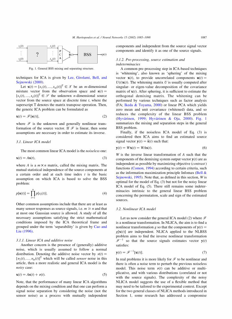
(Hyvarinen, 1999; Hyvarinen & Oja, 2000). Fig. 1

summarizes the mixing and separation steps in the general

BSS problem.

Finally, if the noiseless ICA model of Eq. (3) is

considered then ICA aims to find an estimated source

signal vector yðtÞ ¼ sðtÞ such that:

yðtÞ ¼ WxðtÞ ¼ WAsðtÞ: ð6Þ

W is the inverse linear transformation of A such that the

components of the demixing system output vector yðtÞ are as

independent as possible by maximizing objective (contrast )

functions (Comon, 1994) according to certain criteria, such

as the information maximization principle Infomax (Bell &

Sejnowski, 1995). Note that, as defined in this section, W is

optimal for the model of Eq. (3) but not for the noisy linear

ICA model of Eq. (5). There still remains some indeter-

minacies intrinsic to the general linear BSS problem

concerning the permutation, scale and sign of the estimated

sources.

3.2. Nonlinear ICA model

Let us now consider the general ICA model (2) where Fis a nonlinear transformation. In NLICA, the aim is to find a

nonlinear transformation g so that the components of yðtÞ ¼

g½xðtÞ� are independent. NLICA applied to the NLBSS

problem aims to find the inverse nonlinear transformation

F21 so that the source signals estimates vector yðtÞ

satisfies:

yðtÞ ¼ F21½xðtÞ�: ð7Þ

In real problems it is more likely for F to be nonlinear and

there is often a noise term to perturb the previous noiseless

model. This noise term nðtÞ can be additive or multi-

plicative, and with various distributions (correlated or not

with the source signals). The complexity of the noisy

NLICA model suggests the use of a flexible method that

may need to be tailored to the experimental context. Except

for the two general classes of NLICA methods introduced in

Section 1, some research has addressed a compromise

Fig. 1. General BSS mixing and separating structure.

M. Haritopoulos et al. / Neural Networks 15 (2002) 1085–1098 1087

between standard linear and purely NLICA methods, such

as the ICA mixture models introduced by Lee, Lewicki, and

Sejnowski (1999) and the local linear ICA using K-means

clustering presented by Karhunen and Malaroiu (1999). The

first tries to relax the independence assumption of the

generic ICA model. While the second is closely related to

the batch version of the SOM, but standard K-means

clustering is used, because of the fairly small number of

clusters involved.

Various artificial neural networks have also been applied

to the NLBSS problem. The use of multilayer perceptrons

(MLP) motivated by biomedical applications has been

studied by Lee, Koehler, and Orglmeister (1997), while

earlier Burel (1992) employed a two-layer perceptron.

Recently, a RBF network (Tan, Wang, & Zurada, 2001) has

been used to recover the unknown sources from their

nonlinear mixtures in the presence of cross-nonlinearities.

This method appears robust against additive, uniformly

distributed white noise, but a further noise suppression

technique is necessary to denoise the separated source

signals. SOMs have been used by Pajunen et al. (1996) and

Herrmann and Yang (1996) to extract independent com-

ponents from nonlinearly mixed discrete or continuous

sources. The network complexity increases with the number

of neurons while the quantization error (interpolation error,

in the continuous case) cannot be disregarded. Finally, a

special form of nonlinear mixing, post-nonlinear mixing,

was independently proposed by Taleb and Jutten (1997,

1999) and Lee et al. (1997). In this case, the sources are

assumed to be linearly mixed and then transformed by a

nonlinear transfer channel. This parametric approach uses

sigmoidal functions and MLP networks to approximate the

inverse nonlinearity. However, the approach is limited to a

certain class of nonlinear mixtures and can be considered as

fairly restrictive. A generalization to a rather larger class of

functions is given by Hyvarinen and Pajunen (1999) using

the notion of conformal mapping into the complex domain.

We will now focus into the application of a SOM-based

NLICA technique to the image denoising problem, after a

brief revision of the SOM algorithm.

4. The SOM algorithm

The SOM algorithm is based on competitive learning and

transforms an input space of arbitrary dimension using a

topology preserving nonlinear mapping. Each neuron, j,

1 # j # l is connected to the input through a synaptic

weight vector wj ¼ ½wj1;…;wjm�T: At each iteration, SOM

finds the best-matching (winning) neuron v by minimizing

the following cost function:

vðxÞ ¼ arg minjkxðtÞ2 wjk; j ¼ 1;…; l; ð8Þ

where x belongs to an m-dimensional input space, k·kdenotes the Euclidean distance, while the update of the

synaptic weight vectors follows:

wjðt þ 1Þ ¼ wjðtÞ þ aðtÞhj;vðxÞðtÞ½xðtÞ2 wjðtÞ�;

j ¼ 1;…; l;

ð9Þ

where aðtÞ and hj;vðxÞðtÞ designate the learning rate and the

neighbourhood function centred on the winner, respectively.

Although the algorithm is simple, its convergence and

accuracy depend on the selection of the neighbourhood

function, the topology of the output space, a scheme for

decreasing the learning rate parameter, and the total number

of neuronal units. For the experiments described below, we

used the rules proposed by Haykin (1997) for the dynamic

update of a and hj;vðxÞ:

4.1. Continuous SOMs

When dealing with continuous signals, an interpolation

between the winner and its neighbours is necessary to make

the map continuous. Different interpolation types can be

employed. Geometric interpolation (Goppert & Rosenstiel,

1993) uses orthogonal projections, in the n-dimensional

SOM’s output layer, of the vector formed by the

approximation to the exact input onto the one formed by

the approximation of the second best-matching unit. Topo-

logical interpolation (Goppert and Rosenstiel, 1995) is

based on selecting the topological neighbours of the winner,

which is an advantage over the geometrical method unless

there are topological defects on the chosen map.

4.2. SOM in presence of noise

A modified version of the original Kohonen algorithm for

constructing nonlinear data models in the presence of noise

is given by Der et al. (1996), which provides a good

approximation of the principal manifolds modelling the data

distributions in the presence of multiplicative noise. The

novel aspect of this algorithmic scheme is the use of an

individual neighbourhood for each neuron. The width of the

Gaussian neighbourhood functions is adjusted to keep them

near their critical value. By averaging over the deviations of

the input samples from the winning neurons, an estimate of

the manifold in the data space can be obtained. In Section 6,

we show that this modified algorithm outperforms the

original SOM when applied to simulated signals as well as

to test images.

4.3. NLICA using SOMs

The initial results on the application of SOMs to the

NLBSS problem were reported by Pajunen et al. (1996).

Finding an inverse nonlinear transform F21 from Rn ! Rn

is not a trivial problem unless additional constraints are

applied. Here, the authors restricted F to the family of

homeomorphism functions. The desired mapping must be

M. Haritopoulos et al. / Neural Networks 15 (2002) 1085–10981088

topology-preserving, a property which is satisfied if the two

best-matching units of the SOM are connected neighbours.

Definition of topographic functions and a generalization of

the topology preservation property for more general lattice

structures are given by Villmann, Der, Herrmann, and

Martinetz (1997). However, restrictions apply to this

approach. The mixing model is assumed to be linear,

which is then nonlinearly distorted. The further the source

probability density functions (pdf) are from a uniform one

or the stronger the nonlinearities involved in the mixing

process, the more difficult it is to impose a rigorous mapping

of the input data to the nodes of the map. However, for

mildly nonlinearly mixed, sub-Gaussian source signals and

for a rectangular output lattice, it can been shown, at least

heuristically, that the SOM provides a rough approximation

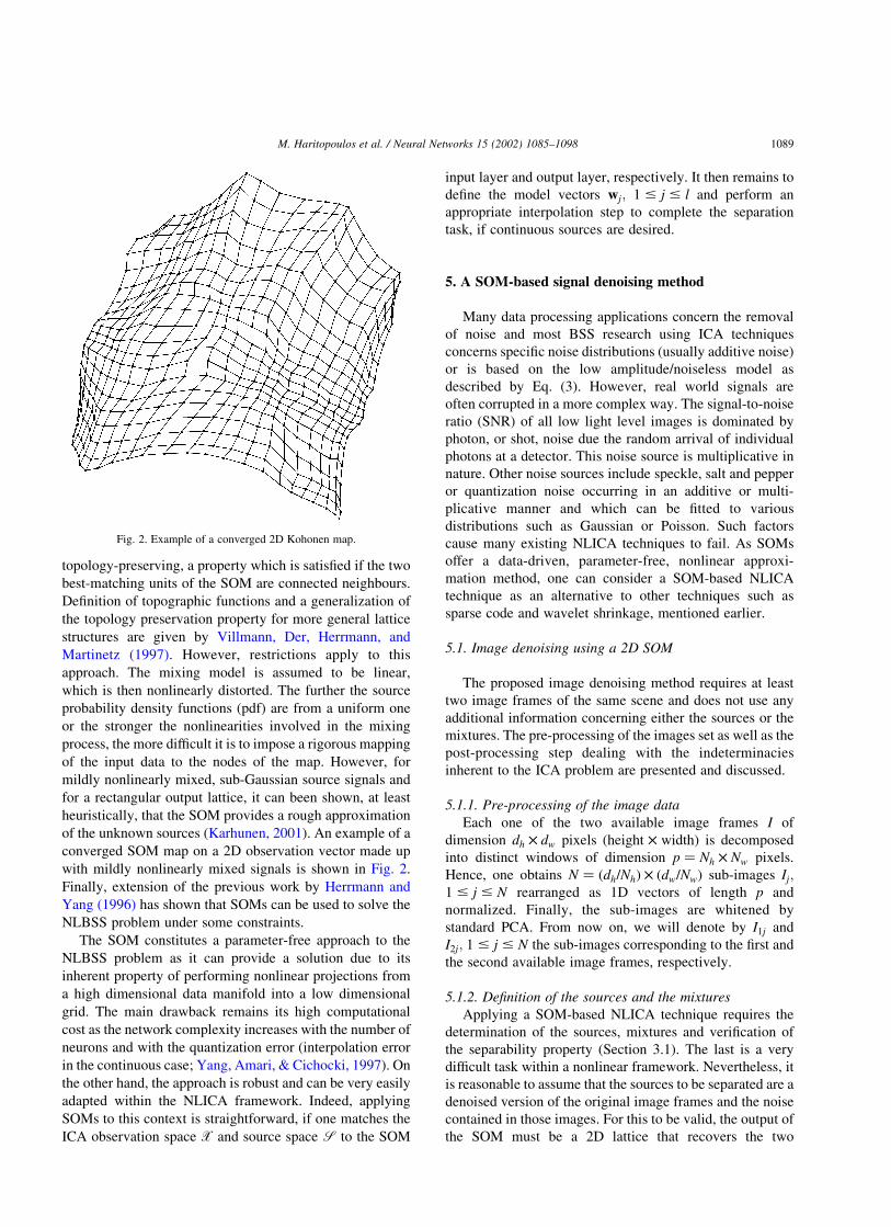
of the unknown sources (Karhunen, 2001). An example of a

converged SOM map on a 2D observation vector made up

with mildly nonlinearly mixed signals is shown in Fig. 2.

Finally, extension of the previous work by Herrmann and

Yang (1996) has shown that SOMs can be used to solve the

NLBSS problem under some constraints.

The SOM constitutes a parameter-free approach to the

NLBSS problem as it can provide a solution due to its

inherent property of performing nonlinear projections from

a high dimensional data manifold into a low dimensional

grid. The main drawback remains its high computational

cost as the network complexity increases with the number of

neurons and with the quantization error (interpolation error

in the continuous case; Yang, Amari, & Cichocki, 1997). On

the other hand, the approach is robust and can be very easily

adapted within the NLICA framework. Indeed, applying

SOMs to this context is straightforward, if one matches the

ICA observation space X and source space S to the SOM

input layer and output layer, respectively. It then remains to

define the model vectors wj; 1 # j # l and perform an

appropriate interpolation step to complete the separation

task, if continuous sources are desired.

5. A SOM-based signal denoising method

Many data processing applications concern the removal

of noise and most BSS research using ICA techniques

concerns specific noise distributions (usually additive noise)

or is based on the low amplitude/noiseless model as

described by Eq. (3). However, real world signals are

often corrupted in a more complex way. The signal-to-noise

ratio (SNR) of all low light level images is dominated by

photon, or shot, noise due the random arrival of individual

photons at a detector. This noise source is multiplicative in

nature. Other noise sources include speckle, salt and pepper

or quantization noise occurring in an additive or multi-

plicative manner and which can be fitted to various

distributions such as Gaussian or Poisson. Such factors

cause many existing NLICA techniques to fail. As SOMs

offer a data-driven, parameter-free, nonlinear approxi-

mation method, one can consider a SOM-based NLICA

technique as an alternative to other techniques such as

sparse code and wavelet shrinkage, mentioned earlier.

5.1. Image denoising using a 2D SOM

The proposed image denoising method requires at least

two image frames of the same scene and does not use any

additional information concerning either the sources or the

mixtures. The pre-processing of the images set as well as the

post-processing step dealing with the indeterminacies

inherent to the ICA problem are presented and discussed.

5.1.1. Pre-processing of the image data

Each one of the two available image frames I of

dimension dh £ dw pixels (height £ width) is decomposed

into distinct windows of dimension p ¼ Nh £ Nw pixels.

Hence, one obtains N ¼ ðdh/NhÞ £ ðdw/NwÞ sub-images Ij;1 # j # N rearranged as 1D vectors of length p and

normalized. Finally, the sub-images are whitened by

standard PCA. From now on, we will denote by I1j and

I2j; 1 # j # N the sub-images corresponding to the first and

the second available image frames, respectively.

5.1.2. Definition of the sources and the mixtures

Applying a SOM-based NLICA technique requires the

determination of the sources, mixtures and verification of

the separability property (Section 3.1). The last is a very

difficult task within a nonlinear framework. Nevertheless, it

is reasonable to assume that the sources to be separated are a

denoised version of the original image frames and the noise

contained in those images. For this to be valid, the output of

the SOM must be a 2D lattice that recovers the two

Fig. 2. Example of a converged 2D Kohonen map.

M. Haritopoulos et al. / Neural Networks 15 (2002) 1085–1098 1089

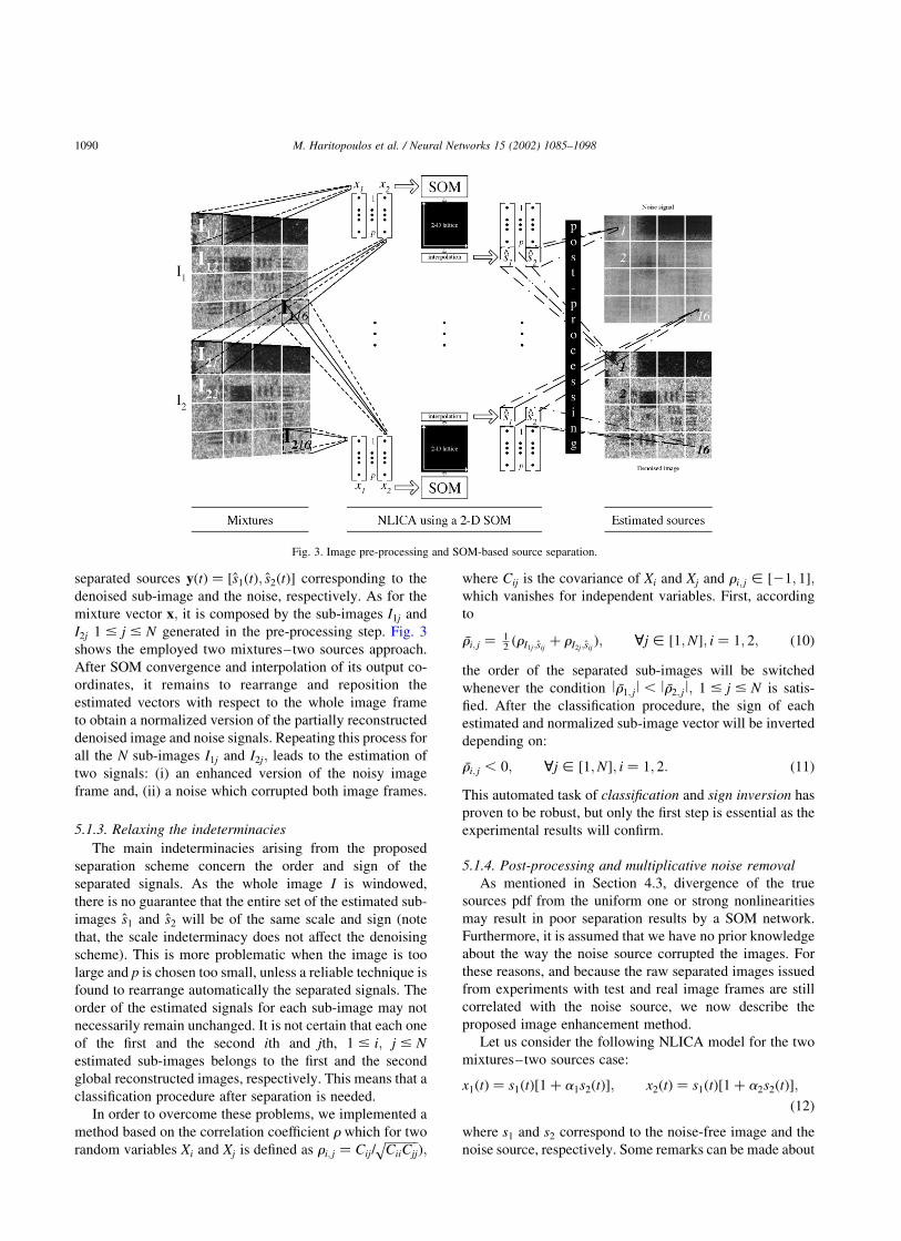
separated sources yðtÞ ¼ ½s1ðtÞ; s2ðtÞ� corresponding to the

denoised sub-image and the noise, respectively. As for the

mixture vector x; it is composed by the sub-images I1j and

I2j 1 # j # N generated in the pre-processing step. Fig. 3

shows the employed two mixtures–two sources approach.

After SOM convergence and interpolation of its output co-

ordinates, it remains to rearrange and reposition the

estimated vectors with respect to the whole image frame

to obtain a normalized version of the partially reconstructed

denoised image and noise signals. Repeating this process for

all the N sub-images I1j and I2j; leads to the estimation of

two signals: (i) an enhanced version of the noisy image

frame and, (ii) a noise which corrupted both image frames.

5.1.3. Relaxing the indeterminacies

The main indeterminacies arising from the proposed

separation scheme concern the order and sign of the

separated signals. As the whole image I is windowed,

there is no guarantee that the entire set of the estimated sub-

images s1 and s2 will be of the same scale and sign (note

that, the scale indeterminacy does not affect the denoising

scheme). This is more problematic when the image is too

large and p is chosen too small, unless a reliable technique is

found to rearrange automatically the separated signals. The

order of the estimated signals for each sub-image may not

necessarily remain unchanged. It is not certain that each one

of the first and the second ith and jth, 1 # i; j # N

estimated sub-images belongs to the first and the second

global reconstructed images, respectively. This means that a

classification procedure after separation is needed.

In order to overcome these problems, we implemented a

method based on the correlation coefficient r which for two

random variables Xi and Xj is defined as ri; j ¼ Cij/ffiffiffiffiffiffiffiCiiCjj

pÞ;

where Cij is the covariance of Xi and Xj and ri; j [ ½21; 1�;which vanishes for independent variables. First, according

to

�ri; j ¼12ðrI1j;sij

þ rI2j;sijÞ; ;j [ ½1;N�; i ¼ 1; 2; ð10Þ

the order of the separated sub-images will be switched

whenever the condition l �r1; jl , l �r2; jl; 1 # j # N is satis-

fied. After the classification procedure, the sign of each

estimated and normalized sub-image vector will be inverted

depending on:

�ri; j , 0; ;j [ ½1;N�; i ¼ 1; 2: ð11Þ

This automated task of classification and sign inversion has

proven to be robust, but only the first step is essential as the

experimental results will confirm.

5.1.4. Post-processing and multiplicative noise removal

As mentioned in Section 4.3, divergence of the true

sources pdf from the uniform one or strong nonlinearities

may result in poor separation results by a SOM network.

Furthermore, it is assumed that we have no prior knowledge

about the way the noise source corrupted the images. For

these reasons, and because the raw separated images issued

from experiments with test and real image frames are still

correlated with the noise source, we now describe the

proposed image enhancement method.

Let us consider the following NLICA model for the two

mixtures–two sources case:

x1ðtÞ ¼ s1ðtÞ½1 þ a1s2ðtÞ�; x2ðtÞ ¼ s1ðtÞ½1 þ a2s2ðtÞ�;

ð12Þ

where s1 and s2 correspond to the noise-free image and the

noise source, respectively. Some remarks can be made about

Fig. 3. Image pre-processing and SOM-based source separation.

M. Haritopoulos et al. / Neural Networks 15 (2002) 1085–10981090

this model. First, it assumes that the noise component s2 is

common to both sources and that only its contribution varies

from frame to frame. Moreover, one could complete the

previous model by a noise term n corresponding to the

sensor noise (see Section 3.1.1) which can be additive (e.g.

thermal noise, quantization noise), multiplicative (e.g.

speckle) or which can corrupt the image in a more complex

way. In the absence of any prior knowledge concerning the

noise, we considered the simplified model of Eq. (12) that

we validated by experiments on test and real images.

After convergence of the SOM network and assuming

that the SOM approximated well the inverse nonlinear

transformation, we obtain the estimated noise-free image s1:But, experiments have shown that some sub-image parts of

s1 still remain noisy after separation. So, we enhance each

one of the noisy frames by adding (subtracting) a slightly

increasing quantity a ¼ {a1;a2} of the normalized esti-

mated noise source s2 to (from) the available noisy image

frames. This can be formulated by:

s11ðtÞ ¼ x1ðtÞ½1 ^ a1s2ðtÞ�21;

s12ðtÞ ¼ x2ðtÞ½1 ^ a2s2ðtÞ�21;

ð13Þ

where s11 and s12 are enhanced versions of the first and the

second noisy frames, respectively. A unique denoised image

may be obtained by averaging over s11 and s12: The

coefficients aopt are optimal in the peak signal-to-noise ratio

(PSNR) sense, defined as:

PSNR ¼ 10 log10

p2max

MSE

!; ð14Þ

where pmax is the maximum value of the image pixel

intensity and MSE denotes the mean-squared error between

the original image and its estimate. However, this requires

additional knowledge concerning the noise-free image

(Hoyer, 1999). For real image denoising, aopt is determined

empirically.

6. Experiments

In this section, we first compare the performances of the

SOM algorithm and its modified version on simulated

nonlinear mixtures as well as test images. Then we apply the

previously described SOM-based image denoising scheme

to real images, together with a performance analysis of the

proposed approach. Note also that for all of our experiments

we used greyscale images.

6.1. Simulation on continuous sources

In order to compare the performances of the original

SOM algorithm (Section 4) and its modified version

(Section 4.2), which will be denoted by SOM-m, we carried

out simulations using the same signal sources as given by

Pajunen et al. (1996). The first source s1 is a sinusoid and the

second source s2 a uniformly distributed white noise. These

sub-Gaussian signals were first mixed linearly with matrix

A ¼0:7 0:3

0:3 0:7

" #;

whose determinant has a value of 0.4 ensuring the well

conditioning of the mixing, providing thus the observation

vector x ðm ¼ 2Þ: This vector was next transformed

nonlinearly by using:

FðxÞ ¼ x3 þ x: ð15Þ

Clearly, the observations are obtained as post-nonlinear

mixtures of the sources: x ¼ FðAsÞ (Taleb & Jutten, 1999).

Finally, they were corrupted with multiplicative noise n of

arbitrary variance s2; generated randomly from a uniform

distribution.

Table 1 summarizes the results of this simulation, where

s1; s2 denote the sinusoid and the white noise sources and

their estimates, respectively. Some experiments also

employed a PCA pre-processing before applying the

SOM-based NLBSS method and used the SNR to quantify

the separation results.

For the source of interest being s1; it can be observed that

in the absence of a pre-whitening step and excepting the

case of small noise variance (s2 ¼ 0:01), SOM-m greatly

enhances the SNR. While, when applying a PCA pre-

treatment to the mixtures, the locally varying neighbour-

hood width of the SOM-m algorithm in conjunction with the

presence of noise helps the map during training to escape

from local minima. Nevertheless, due to the correlation of

the noise with each of the source signals, the estimated

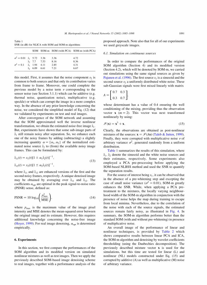
sources remain fairly noisy, as illustrated in Fig. 4. In

summary, the SOM-m algorithm performs better than the

standard SOM (with and without pre-whitening) in presence

of multiplicative noise.

An overall image of the performance of linear and

nonlinear techniques, is provided by Table 2 which

shows comparative results between linear PCA and ICA,

the SOM-m algorithm and denoising by wavelet coefficients

thresholding (using the Daubechies decomposition). The

previously described mixture vector x is used for the

simulations, but this time are tested for linear (L) and

nonlinear (NL) models constructed under Eq. (15) and

corrupted by additive (A) as well as multiplicative (M) noise

of arbitrary variance.

Table 1

SNR (in dB) for NLICA with SOM and SOM-m algorithms

SOM SOM-m SOM (with PCA) SOM-m (with PCA)

s2 ¼ 0:01 s1 5.72 3.36 3.36 4.72

s2 7.7 7.53 8.16 8.36

s2 ¼ 0:1 s1 1.94 4.11 2.85 4.31

s2 6.09 6.61 7.21 6.67

M. Haritopoulos et al. / Neural Networks 15 (2002) 1085–1098 1091

In the NL case, linear methods like PCA and ICA (the

JADE algorithm (Cardoso & Souloumiac, 1993)) perform

poorly; the SNR is relatively close to the one provided by

SOM-m, but clearly, the estimated signal s1 is very different

from the original one. The same is valid for the wavelets

method applied to denoise one of the nonlinear mixtures,

which leads to signals with very smooth waveforms

containing sharp peaks, increasing thus the SNR. On the

contrary, estimation of the useful signal from linear

mixtures improves the SNR for all the proposed methods,

while the best results are provided by the JADE algorithm.

These results confirm that nonlinear methods like SOM-

based algorithms can be very useful in signal estimation and

denoising.

6.2. Image denoising and comparison

Our first image set is a 50 £ 100 pixel region of the Lena

image, containing representative features with high contrast

and which constituted the first source. The second one is a

uniformly distributed random noise of zero mean and

arbitrary variance. These two sources, supposed unknown,

were mixed in a multiplicative manner, using noise

variances of 0.05 and 0.01 to form the observations

consisting of two noisy versions of the Lena image.

The mixing was constructed according Eq. (12) with a1 ¼

a2 ¼ 1:A Nh £ Nw pixels size windowing is used to decompose

each noisy image into an N dimensional vector containing p

samples each (see Section 5.1.1 for notations). To each one

of the sub-images I1j and I2j; 1 # j # N of the whitened 2D

observation vector we apply the SOM-based separation

scheme. Thus, we obtain the estimated source vector y

whose components s1ðtÞ and s2ðtÞ correspond to the

denoised image and the noise source, respectively, after

the classification and sign inversion steps (Section 5.1.3)

and the noise removal procedure (Section 5.1.4).

As the original SOM algorithm does not cope with the

multiplicative noise as well as its modified version SOM-m,

we present here the denoising results obtained using the

latter. Fig. 5 shows the original image and the two separated

signals after interpolation and before removing the indeter-

minacies. They were computed by the SOM-m based

Fig. 4. The observations (left column) and the estimated sources (dotted) obtained by SOM-m in presence of multiplicative noise together with the original ones

(right column).

Table 2

SNR (in dB) for the estimated sinusoid by linear and nonlinear methods

applied to linear (L) and nonlinear (NL) mixture models corrupted by

additive (A) and multiplicative (M) noise of variance s2

Model s2 SOM-m

(with PCA)

Linear ICA Linear PCA Wavelets

L þ A 0.01 10.29 14.45 9.63 9.34

L þ A 0.1 10.44 12.69 9.33 8.39

NL þ M 0.01 4.72 3.51 4.02 5.73

NL þ M 0.1 4.31 3.94 2.89 4.77

L þ M 0.01 6.35 14.44 9.64 13.49

L þ M 0.1 9.37 13.1 9.53 13.24

NL þ A 0.01 4.11 3.38 4.06 5.81

NL þ A 0.1 2.91 2.92 3.83 5.49

M. Haritopoulos et al. / Neural Networks 15 (2002) 1085–10981092

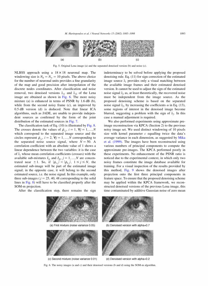
NLBSS approach using a 18 £ 18 neuronal map. The

windowing size is Nh ¼ Nw ¼ 10 pixels. The above choice

for the number of neuronal units provides a fine granularity

of the map and good precision after interpolation of the

discrete nodes coordinates. After classification and noise

removal, two denoised versions s11 and s12 of the Lena

image are obtained as shown in Fig. 6. The more noisy

mixture (a) is enhanced in terms of PSNR by 1.6 dB (b),

while from the second noisy frame (c), an improved by

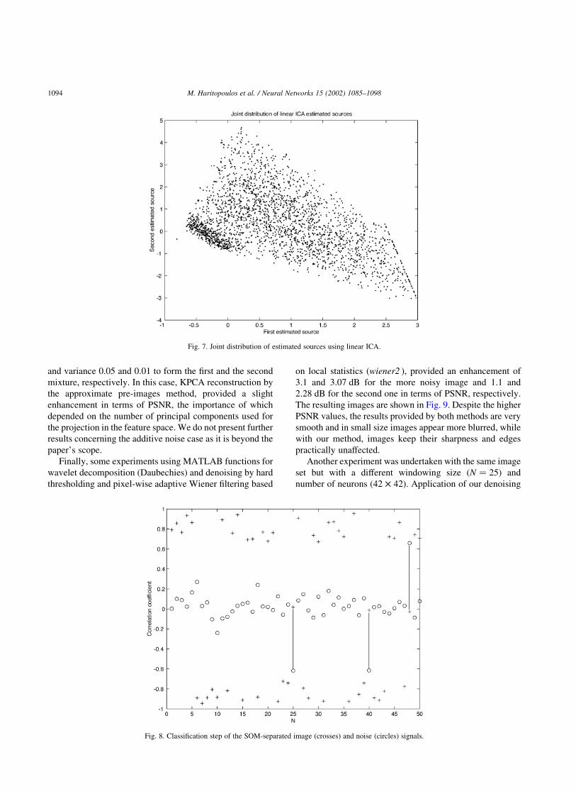
0.5 dB version (d) is deduced. Note that linear ICA

algorithms, such as JADE, are unable to provide indepen-

dent sources as confirmed by the form of the joint

distribution of the estimated sources in Fig. 7.

The classification task of Eq. (10) is illustrated by Fig. 8.

The crosses denote the values of �ri; j; i ¼ 1; ;j ¼ 1;…;N

which correspond to the separated image source and the

circles represent �ri; j; i ¼ 2; ;j ¼ 1;…;N corresponding to

the separated noise source signal, where N ¼ 50: A

correlation coefficient with an absolute value of 1 shows a

linear dependence between the two variables: it is the case

of s1 whose mean correlation coefficients (crosses) with the

available sub-mixtures I1j and I2j; j ¼ 1;…;N are concen-

trated near ^1. So, if l �r1; jl a l �r2; jl; 1 # j # N; the

estimated sub-image will be part of the estimated image

signal; in the opposite case, it will belong to the second

estimated source, i.e. the noise signal. In this example, only

three sub-images ( j ¼ 25; 40, 48 corresponding to the solid

lines in Fig. 8) will have to be classified properly after the

SOM-m projection.

After the classification step, there remains the sign

indeterminacy to be solved before applying the proposed

denoising rule. Eq. (11) for sign correction of the estimated

image source s1 provides only a visual matching between

the available image frames and their estimated denoised

version. It cannot be used to adjust the sign of the estimated

noise signal s2 as, at least theoretically, the recovered noise

must be independent from the image source. As the

proposed denoising scheme is based on the separated

noise signal s2; by increasing the coefficients a in Eq. (13),

some regions of interest in the denoised image become

blurred, suggesting a problem with the sign of s2: In this

case a manual adjustment is required.

We also performed experiments using approximate pre-

image reconstruction via KPCA (Section 2) to the previous

noisy image set. We used distinct windowing of 10 pixels

size with kernel parameter c equalling twice the data’s

average variance in each dimension, as suggested by Mika

et al. (1999). The images have been reconstructed using

various numbers of principal components to compute the

approximate pre-images. The KPCA performed poorly in

these experiments. No enhancement of the PSNR ratio is

noticed due to the experimental context, in which only two

noisy frames constitute the image database available for

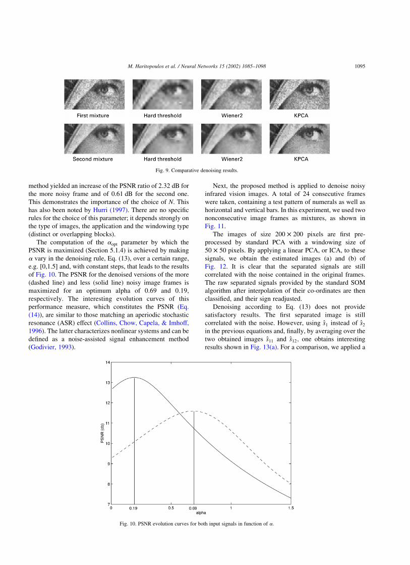
training. For a visual inspection of the results provided by

this method, Fig. 9 shows the denoised images after

projection onto the first three principal components in

feature space. To ensure that the proposed denoising scheme

may be applied within the KPCA framework, we recon-

structed denoised versions of the previous Lena image, this

time contaminated by additive Gaussian noise of zero mean

Fig. 5. Original Lena image (a) and the separated denoised version (b) and noise (c).

Fig. 6. The noisy images (a and c) and their denoised versions (b and d) using the SOM-m algorithm.

M. Haritopoulos et al. / Neural Networks 15 (2002) 1085–1098 1093

and variance 0.05 and 0.01 to form the first and the second

mixture, respectively. In this case, KPCA reconstruction by

the approximate pre-images method, provided a slight

enhancement in terms of PSNR, the importance of which

depended on the number of principal components used for

the projection in the feature space. We do not present further

results concerning the additive noise case as it is beyond the

paper’s scope.

Finally, some experiments using MATLAB functions for

wavelet decomposition (Daubechies) and denoising by hard

thresholding and pixel-wise adaptive Wiener filtering based

on local statistics (wiener2 ), provided an enhancement of

3.1 and 3.07 dB for the more noisy image and 1.1 and

2.28 dB for the second one in terms of PSNR, respectively.

The resulting images are shown in Fig. 9. Despite the higher

PSNR values, the results provided by both methods are very

smooth and in small size images appear more blurred, while

with our method, images keep their sharpness and edges

practically unaffected.

Another experiment was undertaken with the same image

set but with a different windowing size (N ¼ 25) and

number of neurons (42 £ 42). Application of our denoising

Fig. 7. Joint distribution of estimated sources using linear ICA.

Fig. 8. Classification step of the SOM-separated image (crosses) and noise (circles) signals.

M. Haritopoulos et al. / Neural Networks 15 (2002) 1085–10981094

method yielded an increase of the PSNR ratio of 2.32 dB for

the more noisy frame and of 0.61 dB for the second one.

This demonstrates the importance of the choice of N. This

has also been noted by Hurri (1997). There are no specific

rules for the choice of this parameter; it depends strongly on

the type of images, the application and the windowing type

(distinct or overlapping blocks).

The computation of the aopt parameter by which the

PSNR is maximized (Section 5.1.4) is achieved by making

a vary in the denoising rule, Eq. (13), over a certain range,

e.g. [0,1.5] and, with constant steps, that leads to the results

of Fig. 10. The PSNR for the denoised versions of the more

(dashed line) and less (solid line) noisy image frames is

maximized for an optimum alpha of 0.69 and 0.19,

respectively. The interesting evolution curves of this

performance measure, which constitutes the PSNR (Eq.

(14)), are similar to those matching an aperiodic stochastic

resonance (ASR) effect (Collins, Chow, Capela, & Imhoff,

1996). The latter characterizes nonlinear systems and can be

defined as a noise-assisted signal enhancement method

(Godivier, 1993).

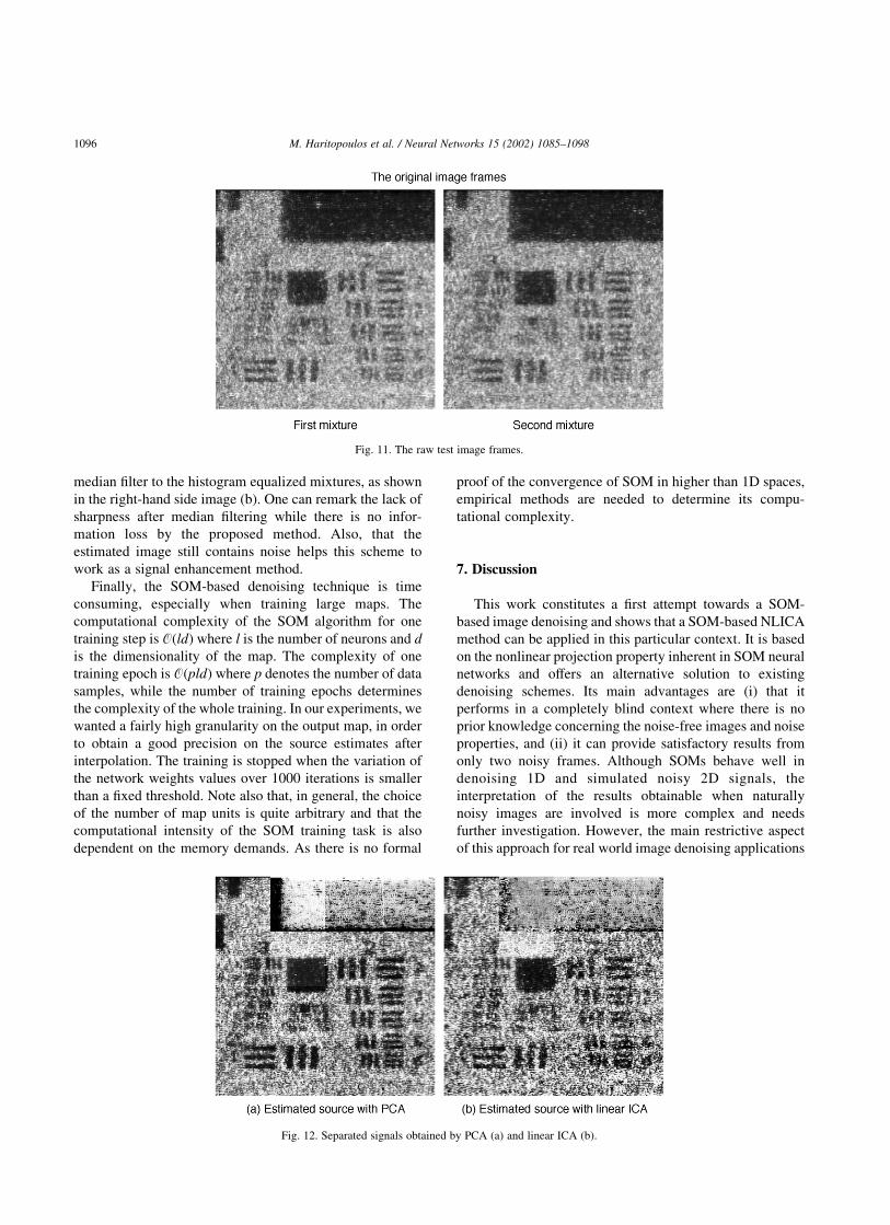
Next, the proposed method is applied to denoise noisy

infrared vision images. A total of 24 consecutive frames

were taken, containing a test pattern of numerals as well as

horizontal and vertical bars. In this experiment, we used two

nonconsecutive image frames as mixtures, as shown in

Fig. 11.

The images of size 200 £ 200 pixels are first pre-

processed by standard PCA with a windowing size of

50 £ 50 pixels. By applying a linear PCA, or ICA, to these

signals, we obtain the estimated images (a) and (b) of

Fig. 12. It is clear that the separated signals are still

correlated with the noise contained in the original frames.

The raw separated signals provided by the standard SOM

algorithm after interpolation of their co-ordinates are then

classified, and their sign readjusted.

Denoising according to Eq. (13) does not provide

satisfactory results. The first separated image is still

correlated with the noise. However, using s1 instead of s2

in the previous equations and, finally, by averaging over the

two obtained images s11 and s12; one obtains interesting

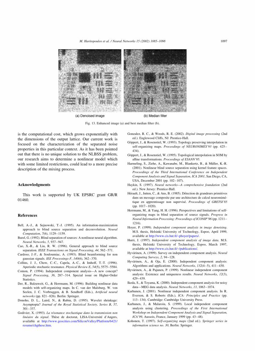
results shown in Fig. 13(a). For a comparison, we applied a

Fig. 9. Comparative denoising results.

Fig. 10. PSNR evolution curves for both input signals in function of a:

M. Haritopoulos et al. / Neural Networks 15 (2002) 1085–1098 1095

median filter to the histogram equalized mixtures, as shown

in the right-hand side image (b). One can remark the lack of

sharpness after median filtering while there is no infor-

mation loss by the proposed method. Also, that the

estimated image still contains noise helps this scheme to

work as a signal enhancement method.

Finally, the SOM-based denoising technique is time

consuming, especially when training large maps. The

computational complexity of the SOM algorithm for one

training step is OðldÞ where l is the number of neurons and d

is the dimensionality of the map. The complexity of one

training epoch is OðpldÞ where p denotes the number of data

samples, while the number of training epochs determines

the complexity of the whole training. In our experiments, we

wanted a fairly high granularity on the output map, in order

to obtain a good precision on the source estimates after

interpolation. The training is stopped when the variation of

the network weights values over 1000 iterations is smaller

than a fixed threshold. Note also that, in general, the choice

of the number of map units is quite arbitrary and that the

computational intensity of the SOM training task is also

dependent on the memory demands. As there is no formal

proof of the convergence of SOM in higher than 1D spaces,

empirical methods are needed to determine its compu-

tational complexity.

7. Discussion

This work constitutes a first attempt towards a SOM-

based image denoising and shows that a SOM-based NLICA

method can be applied in this particular context. It is based

on the nonlinear projection property inherent in SOM neural

networks and offers an alternative solution to existing

denoising schemes. Its main advantages are (i) that it

performs in a completely blind context where there is no

prior knowledge concerning the noise-free images and noise

properties, and (ii) it can provide satisfactory results from

only two noisy frames. Although SOMs behave well in

denoising 1D and simulated noisy 2D signals, the

interpretation of the results obtainable when naturally

noisy images are involved is more complex and needs

further investigation. However, the main restrictive aspect

of this approach for real world image denoising applications

Fig. 11. The raw test image frames.

Fig. 12. Separated signals obtained by PCA (a) and linear ICA (b).

M. Haritopoulos et al. / Neural Networks 15 (2002) 1085–10981096

is the computational cost, which grows exponentially with

the dimensions of the output lattice. Our current work is

focused on the characterization of the separated noise

properties in this particular context. As it has been pointed

out that there is no unique solution to the NLBSS problem,

our research aims to determine a nonlinear model which

with some limited restrictions, could lead to a more precise

description of the mixing process.

Acknowledgments

This work is supported by UK EPSRC grant GR/R

01460.

References

Bell, A.-J., & Sejnowski, T.-J. (1995). An information-maximization

approach to blind source separation and deconvolution. Neural

Computation, 7(6), 1129–1159.

Burel, G. (1992). Blind separation of sources: A nonlinear neural algorithm.

Neural Networks, 5, 937–947.

Cao, X.-R., & Liu, R. W. (1996). General approach to blind source

separation. IEEE Transactions on Signal Processing, 44, 562–571.

Cardoso, J.-F., & Souloumiac, A. (1993). Blind beamforming for non

gaussian signals. IEE Processings-F, 140(6), 362–370.

Collins, J. J., Chow, C.-C., Capela, A.-C., & Imhoff, T.-T. (1996).

Aperiodic stochastic resonance. Physical Review E, 54(5), 5575–5584.

Comon, P. (1994). Independent component analysis—A new concept?

Signal Processing, 36, 287–314. Special issue on Higher-Order

Statistics.

Der, R., Balzuweit, G., & Herrmann, M. (1996). Building nonlinear data

models with self-organizing maps. In C. van der Malsburg, W. von

Seelen, J. C. Vorbruggen, & B. Sendhoff (Eds.), Artificial neural

networks (pp. 821–826). Berlin: Springer.

Donoho, D. L., Laird, N., & Rubin, D. (1995). Wavelet shrinkage:

Asymptopia? Journal of the Royal Statistical Society, Series B, 57,

301–337.

Godivier, X. (1993). La resonance stochastique dans la transmission non

lineaire du signal. These de doctorat, LISA-Universite d’Angers,

available at http://www.geocities.com/SiliconValley/Platform/6421/

resume/chgthese.htm.

Gonzalez, R. C., & Woods, R. E. (2002). Digital image processing (2nd

ed.). Englewood Cliffs, NJ: Prentice-Hall.

Goppert, J., & Rosenstiel, W. (1993). Topology preserving interpolation in

self-organizing maps. Proceedings of NEURONIMES’93 (pp. 425–

434).

Goppert, J., & Rosenstiel, W. (1995). Topological interpolation in SOM by

affine transformations. Proceedings of ESANN’95.

Harmeling, S., Ziehe, A., Kawanabe, M., Blankertz, B., & Muller, K.-R.

(2001). Nonlinear blind source separation using kernel feature spaces.

Proceedings of the Third International Conference on Independent

Component Analysis and Signal Separation, ICA 2001, San Diego, CA,

USA, December 2001 (pp. 102–107).

Haykin, S. (1997). Neural networks—A comprehensive foundation (2nd

ed.). New Jersey: Prentice-Hall.

Herault, J., Jutten, C., & Ans, B. (1985). Detection de grandeurs primitives

dans un message composite par une architecture de calcul neuromime-

tique en apprentissage non supervise. Proceedings of GRETSI’85

(pp. 1017–1020).

Herrmann, M., & Yang, H. H. (1996). Perspectives and limitations of self-

organizing maps in blind separation of source signals. Progress in

Neural Information Processing: Proceedings of ICONIP’96 (pp. 1211–

1216).

Hoyer, P. (1999). Independent component analysis in image denoising.

M.S. thesis, Helsinki University of Technology, Espoo, April 1999,

available at http://www.cis.hut.fi/~phoyer/papers/.

Hurri, J. (1997). Independent component analysis of image data. M.S.

thesis, Helsinki University of Technology, Espoo, March 1997,

available at http://www.cis.hut.fi/~/publications/.

Hyvarinen, A. (1999). Survey on independent component analysis. Neural

Computing Surveys, 2, 94–128.

Hyvarinen, A., & Oja, E. (2000). Independent component analysis:

Algorithms and applications. Neural Networks, 132(4–5), 411–430.

Hyvarinen, A., & Pajunen, P. (1999). Nonlinear independent component

analysis: Existence and uniqueness results. Neural Networks, 12(3),

429–439.

Ikeda, S., & Toyama, K. (2000). Independent component analysis for noisy

data—MEG data analysis. Neural Networks, 13, 1063–1074.

Karhunen, J. (2001). Nonlinear independent component analysis. In R.

Everson, & S. Roberts (Eds.), ICA: Principles and Practice (pp.

113–134). Cambridge: Cambridge University Press.

Karhunen, J., & Malaroiu, S. (1999). Local independent component

analysis using clustering. Proceedings of the First International

Workshop on Independent Component Analysis and Signal Separation,

ICA’99, Aussois, France, January 1999 (pp. 43–48).

Kohonen, T. (1997). Self-organizing maps (2nd ed.). Springer series in

information science no. 30, Berlin: Springer.

Fig. 13. Enhanced image (a) and best median filter (b).

M. Haritopoulos et al. / Neural Networks 15 (2002) 1085–1098 1097

Lee, T.-W. (1999). Nonlinear approaches to independent component

analysis. Proceedings of American Institute of Physics.

Lee, T.-W., Girolami, M., Bell, A.-J., & Sejnowski, T.-J. (2000). A unifying

information—Theoretic framework for independent component analy-

sis. Computers and Mathematics with Applications, 31(11), 1–21.

Lee, T.-W., Koehler, B.-U., & Orglmeister, R. (1997). Blind source

separation of nonlinear mixing models. In J. Principe, L. Gile, N.

Morgan, & E. Wilson (Eds.), Proceedings of 1997 IEEE Workshop,

Neural Networks for Signal Processing VII, NNSP’97 (pp. 406–415).

New York: IEEE Press.

Lee, T.-W., Lewicki, M.-S., & Sejnowski, T.-J. (1999). Unsupervised

classification with non-Gaussian mixture models using ICA. Advances

in Neural Information Processing Systems, 11, 508–514.

Mallat, S. G. (1989). A theory for multiresolution signal decomposition:

The wavelet representation. IEEE Transactions on Pattern Analysis and

Machine Intelligence, 11, 674–693.

Mika, S., Scholkopf, B., Smola, A., Muller, K.-R., Scholz, M., & Ratsch, G.

(1999). Kernel PCA and de-noising in feature spaces. Advances in

Neural Information Processing Systems, 11, 536–542.

Muller, K.-R., Mika, S., Ratsch, G., Tsuda, K., & Scholkopf, B. (2001). An

introduction to kernel-based learning algorithms. IEEE Transactions on

Neural Networks, 12(2), 181–201.

Pajunen, P., Hyvarinen, A., & Karhunen, J. (1996). Nonlinear blind source

separation by self-organizing maps. Progress in Neural Information

Processing: Proceedings of ICONIP’96, Hong-Kong (pp. 1207–1210).

Scholkopf, B., Mika, S., Burges, C. J. C., Knirsch, P., Muller, K.-R., Ratsch,

G., & Smola, A. J. (1999). Input space versus feature space in kernel-

based methods. IEEE Transactions on Neural Networks, 10,

1000–1017.

Scholkopf, B., Mika, S., Smola, A. J., Ratsch, G., & Muller, K.-G. (1998).

Kernel PCA pattern reconstruction via approximate pre-images. In M.

Bodn, L. Niklasson, & T. Ziemke (Eds.), Perspectives in Neural

Computing: Proceedings of the 8th International Conference on

Artificial Neural Networks (pp. 147–152). Berlin: Springer.

Scholkopf, B., Smola, A. J., & Muller, K.-R. (1999). Nonlinear component

analysis as a kernel eigenvalue problem. Neural Computation, 10,

1299–1319.

Taleb, A., & Jutten, C. (1997). Nonlinear source separation: The post-

nonlinear mixtures. Proceedings of European Symposium on Artificial

Neural Networks, ESANN’97, Bruges, Belgium, April 1997 (pp. 279–

284).

Taleb, A., & Jutten, C. (1999). Source separation in postnonlinear mixtures.

IEEE Transactions on Signal Processing, 47(10), 2807–2820.

Tan, Y., Wang, J., & Zurada, J. M. (2001). Nonlinear blind source

separation using a radial basis function network. IEEE Transactions on

Neural Networks, 12(1), 124–134.

Villmann, T., Der, R., Herrmann, M., & Martinetz, T. M. (1997). Topology

preservation in self-organizing feature maps: Exact definition and

measurement. IEEE Transactions on Neural Networks, 8(2), 256–266.

Weyrich, N., & Warhola, T. (1998). Wavelet shrinkage and generalized

cross validation for image denoising. IEEE Transactions on Image

Processing, 7(1), 82–90.

Yang, H. H., Amari, S., & Cichocki, A. (1997). Information back-

propagation for blind separation of sources in non-linear mixture.

Proceedings of IEEE ICNN’97 (pp. 2141–2146).

M. Haritopoulos et al. / Neural Networks 15 (2002) 1085–10981098