Embed Size (px)
Citation preview

2005 Hopkins Epi-Biostat Summer Institute 1
Module 2: Bayesian Hierarchical Models
Francesca Dominici
Michael Griswold
The Johns Hopkins University
Bloomberg School of Public Health
2005 Hopkins Epi-Biostat Summer Institute 2
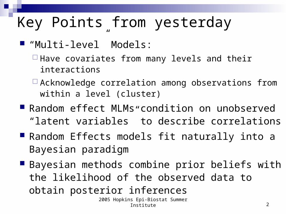
Key Points from yesterday
“Multi-level” Models: Have covariates from many levels and their interactions Acknowledge correlation among observations from
within a level (cluster)
Random effect MLMs condition on unobserved “latent variables” to describe correlations
Random Effects models fit naturally into a Bayesian paradigm
Bayesian methods combine prior beliefs with the likelihood of the observed data to obtain posterior inferences
2005 Hopkins Epi-Biostat Summer Institute 3
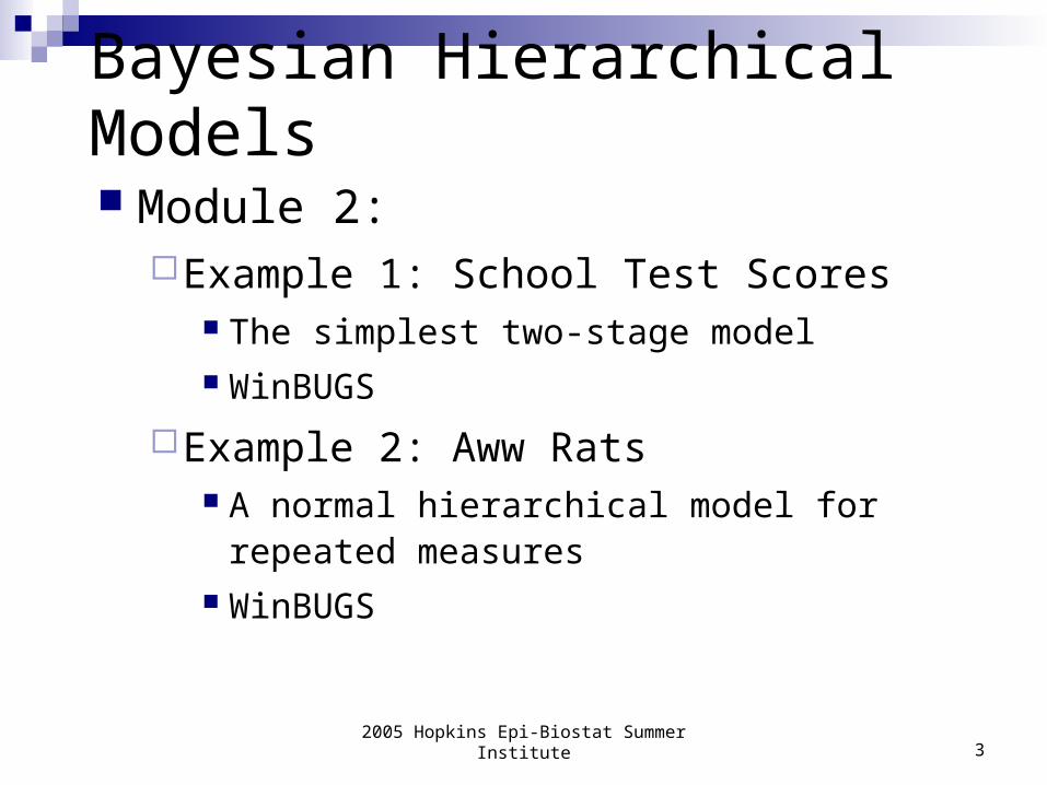
Bayesian Hierarchical Models
Module 2:Example 1: School Test Scores
The simplest two-stage model WinBUGS
Example 2: Aww Rats A normal hierarchical model for repeated
measures WinBUGS
2005 Hopkins Epi-Biostat Summer Institute 4
Example 1: School Test Scores
2005 Hopkins Epi-Biostat Summer Institute 5
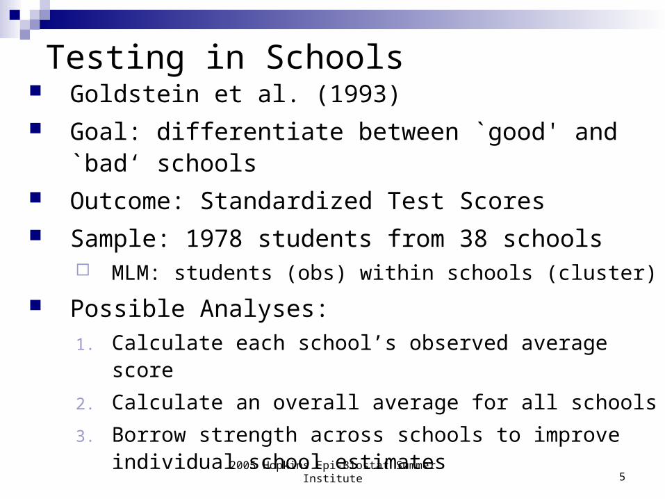
Testing in Schools Goldstein et al. (1993) Goal: differentiate between `good' and `bad‘
schools Outcome: Standardized Test Scores Sample: 1978 students from 38 schools
MLM: students (obs) within schools (cluster)
Possible Analyses:1. Calculate each school’s observed average score
2. Calculate an overall average for all schools
3. Borrow strength across schools to improve individual school estimates
2005 Hopkins Epi-Biostat Summer Institute 6
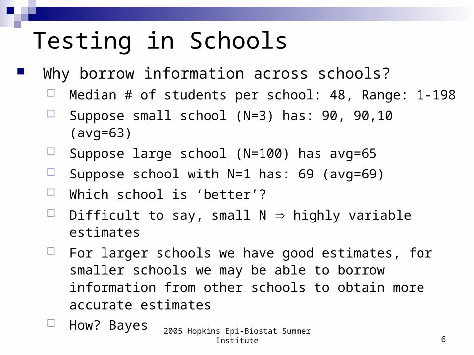
Testing in Schools Why borrow information across schools?
Median # of students per school: 48, Range: 1-198 Suppose small school (N=3) has: 90, 90,10 (avg=63) Suppose large school (N=100) has avg=65 Suppose school with N=1 has: 69 (avg=69) Which school is ‘better’? Difficult to say, small N highly variable estimates For larger schools we have good estimates, for
smaller schools we may be able to borrow information from other schools to obtain more accurate estimates
How? Bayes
2005 Hopkins Epi-Biostat Summer Institute 7
0 10 20 30 40
02
04
06
08
01
00
school
sco
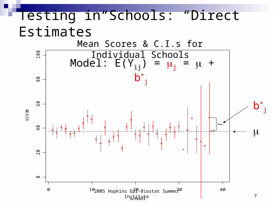
reTesting in Schools: “Direct Estimates”
Model: E(Yij) = j = + b*j
Mean Scores & C.I.s for Individual Schools
b*j
2005 Hopkins Epi-Biostat Summer Institute 8
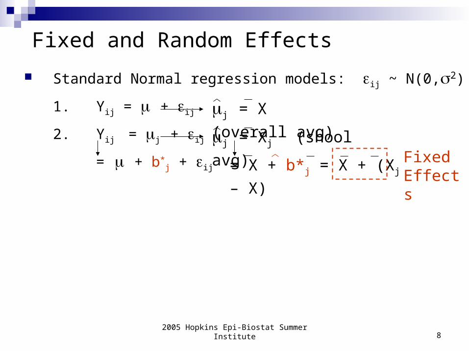
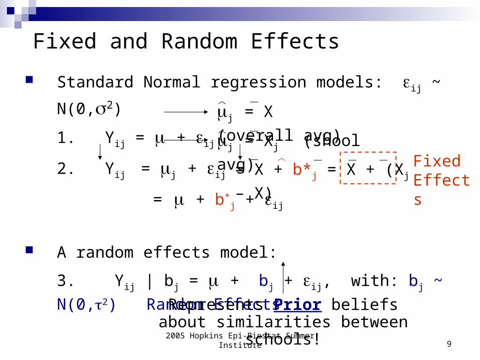
Standard Normal regression models: ij ~ N(0,2)
1. Yij = + ij
2. Yij = j + ij
= + b*j + ij
Fixed and Random Effects
j = X (overall avg)
j = Xj (shool avg)
= X + b*j = X + (Xj – X) Fixed Effects
2005 Hopkins Epi-Biostat Summer Institute 9
Standard Normal regression models: ij ~ N(0,2)
1. Yij = + ij
2. Yij = j + ij
= + b*j + ij
A random effects model:
3. Yij | bj = + bj + ij, with: bj ~ N(0,2) Random
Effects
Fixed and Random Effects
j = X (overall avg)
j = Xj (shool avg)
= X + b*j = X + (Xj – X) Fixed Effects
Represents Prior beliefs about similarities between schools!
2005 Hopkins Epi-Biostat Summer Institute 10
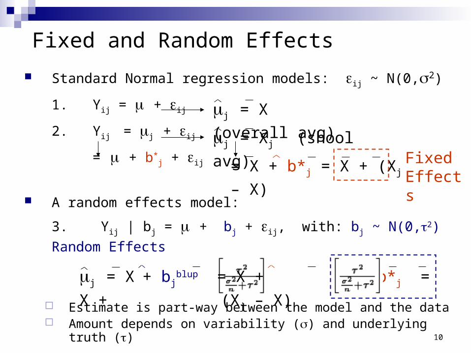
Standard Normal regression models: ij ~ N(0,2)
1. Yij = + ij
2. Yij = j + ij
= + b*j + ij
A random effects model:
3. Yij | bj = + bj + ij, with: bj ~ N(0,2) Random
Effects
Estimate is part-way between the model and the data Amount depends on variability () and underlying truth ()
Fixed and Random Effects
j = X (overall avg)
j = Xj (shool avg)
j = X + bjblup = X + b*j = X + (Xj – X)
= X + b*j = X + (Xj – X) Fixed Effects
2005 Hopkins Epi-Biostat Summer Institute 11
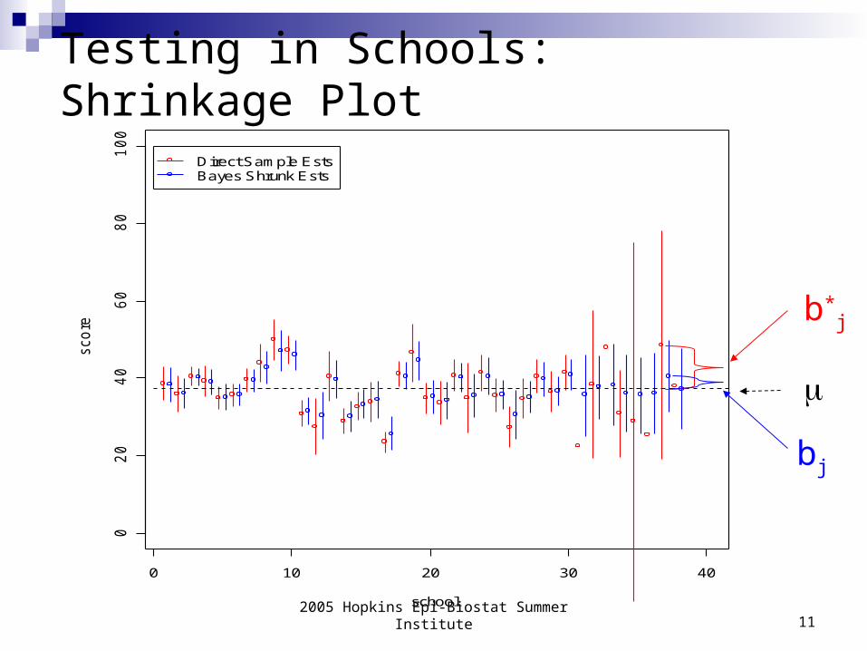
Testing in Schools: Shrinkage Plot
0 10 20 30 40
02
04
06
08
01
00
school
sco
re
Direct Sample EstsBayes Shrunk Ests
b*j
bj
2005 Hopkins Epi-Biostat Summer Institute 12
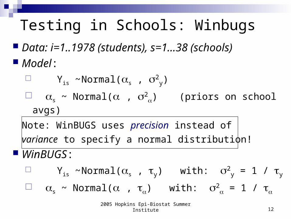
Testing in Schools: Winbugs
Data: i=1..1978 (students), s=1…38 (schools) Model:
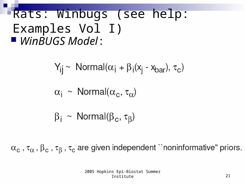
Yis ~ Normal(s , 2y)
s ~ Normal( , 2) (priors on school avgs)
Note: WinBUGS uses precision instead of
variance to specify a normal distribution! WinBUGS:
Yis ~ Normal(s , y) with: 2y = 1 / y
s ~ Normal( , ) with: 2 = 1 /
2005 Hopkins Epi-Biostat Summer Institute 13
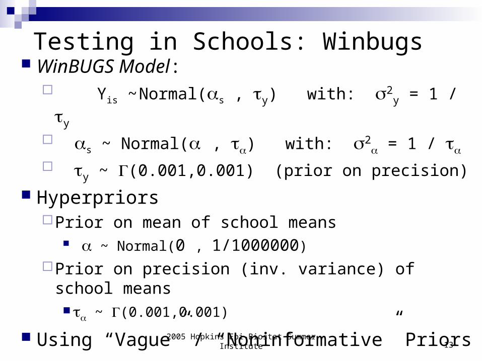
Testing in Schools: Winbugs WinBUGS Model:
Yis ~ Normal(s , y) with: 2y = 1 / y
s ~ Normal( , ) with: 2 = 1 /
y ~ (0.001,0.001) (prior on precision)
HyperpriorsPrior on mean of school means
~ Normal(0 , 1/1000000)
Prior on precision (inv. variance) of school means ~ (0.001,0.001)
Using “Vague” / “Noninformative” Priors
2005 Hopkins Epi-Biostat Summer Institute 14
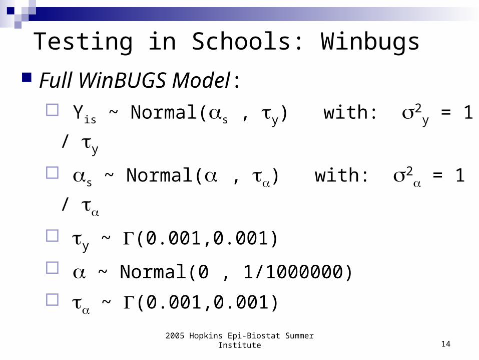
Testing in Schools: Winbugs
Full WinBUGS Model: Yis ~ Normal(s , y) with: 2
y = 1 / y
s ~ Normal( , ) with: 2 = 1 /
y ~ (0.001,0.001)
~ Normal(0 , 1/1000000)
~ (0.001,0.001)
2005 Hopkins Epi-Biostat Summer Institute 15
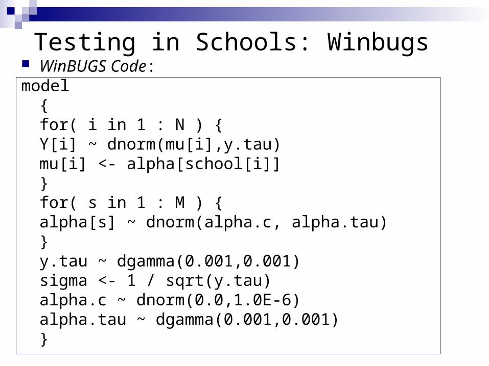
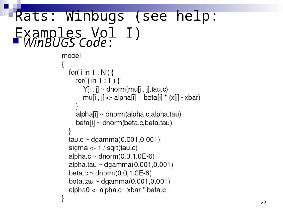
Testing in Schools: Winbugs WinBUGS Code:model
{for( i in 1 : N ) {
Y[i] ~ dnorm(mu[i],y.tau)mu[i] <- alpha[school[i]] }
for( s in 1 : M ) {alpha[s] ~ dnorm(alpha.c, alpha.tau)}
y.tau ~ dgamma(0.001,0.001)sigma <- 1 / sqrt(y.tau)alpha.c ~ dnorm(0.0,1.0E-6)alpha.tau ~ dgamma(0.001,0.001)
}
2005 Hopkins Epi-Biostat Summer Institute 16
Example 2: Aww, Rats…A normal hierarchical model for
repeated measures
2005 Hopkins Epi-Biostat Summer Institute 17
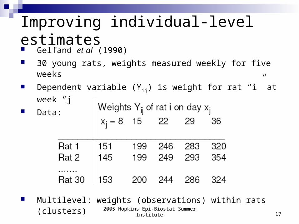
Improving individual-level estimates Gelfand et al (1990) 30 young rats, weights measured weekly for five weeks
Dependent variable (Yij) is weight for rat “i” at week “j”
Data:
Multilevel: weights (observations) within rats (clusters)
2005 Hopkins Epi-Biostat Summer Institute 18
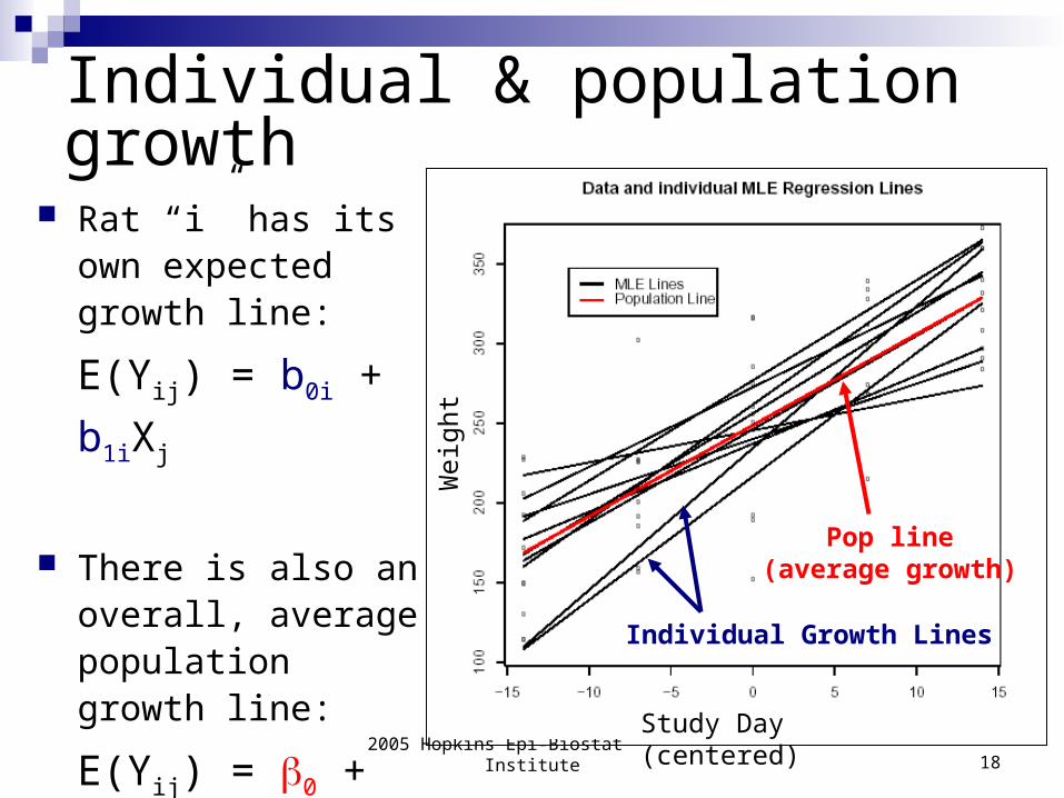
Individual & population growth
Pop line(average growth)
Individual Growth Lines
Rat “i” has its own expected growth line:
E(Yij) = b0i + b1iXj
There is also an overall, average population growth line:
E(Yij) = 0 + 1Xj
Wei
ght
Study Day (centered)
2005 Hopkins Epi-Biostat Summer Institute 19
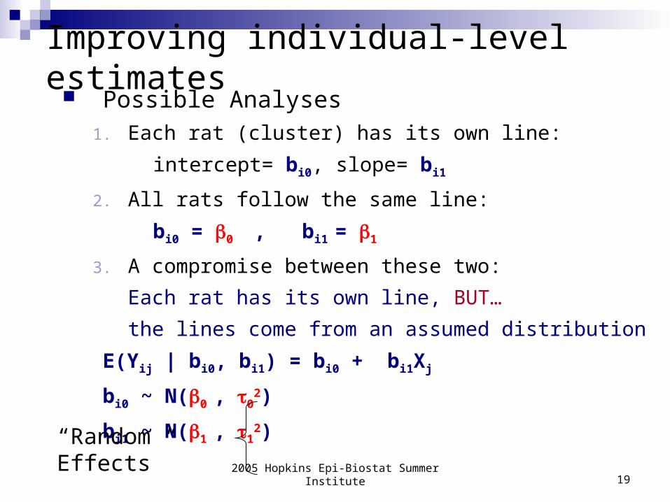
Improving individual-level estimates Possible Analyses
1. Each rat (cluster) has its own line:
intercept= bi0, slope= bi1
2. All rats follow the same line:
bi0 = 0 , bi1 = 1
3. A compromise between these two:
Each rat has its own line, BUT…
the lines come from an assumed distribution
E(Yij | bi0, bi1) = bi0 + bi1Xj
bi0 ~ N(0 , 02)
bi1 ~ N(1 , 12)“Random Effects”
2005 Hopkins Epi-Biostat Summer Institute 20
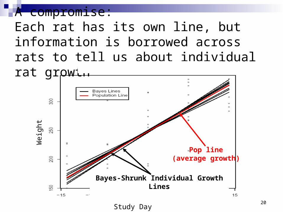
Pop line(average growth)
Bayes-Shrunk Individual Growth Lines
A compromise: Each rat has its own line, but information is borrowed across rats to tell us about individual rat growth
Wei
ght
Study Day (centered)
2005 Hopkins Epi-Biostat Summer Institute 21
Rats: Winbugs (see help: Examples Vol I)
WinBUGS Model:
2005 Hopkins Epi-Biostat Summer Institute 22
Rats: Winbugs (see help: Examples Vol I) WinBUGS Code:
2005 Hopkins Epi-Biostat Summer Institute 23
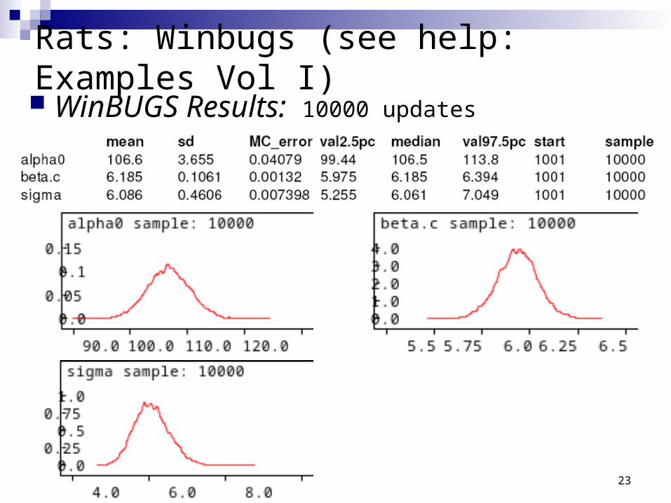
Rats: Winbugs (see help: Examples Vol I) WinBUGS Results: 10000 updates
2005 Hopkins Epi-Biostat Summer Institute 24
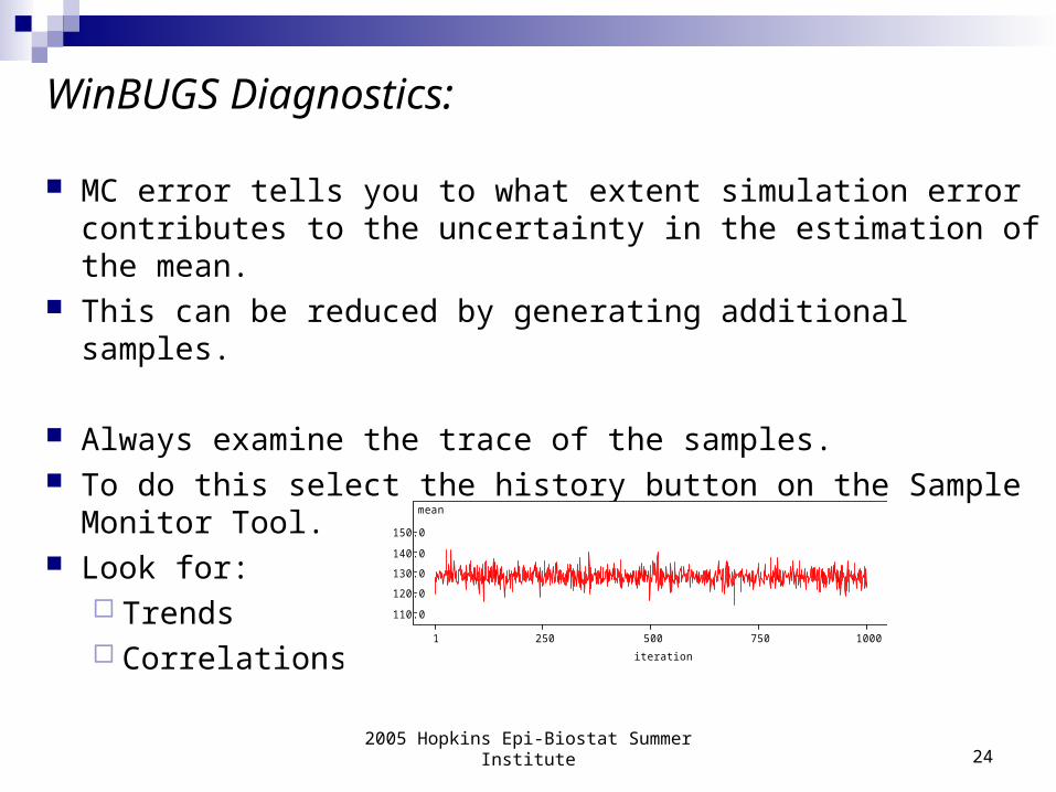
WinBUGS Diagnostics:
MC error tells you to what extent simulation error contributes to the uncertainty in the estimation of the mean.
This can be reduced by generating additional samples.
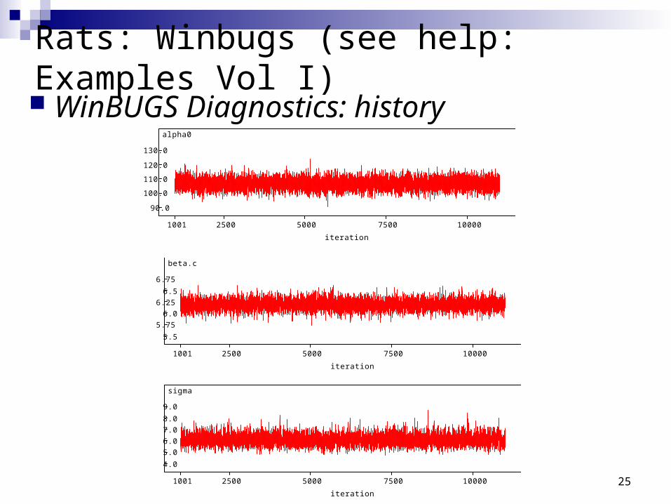
Always examine the trace of the samples. To do this select the history button on the Sample Monitor
Tool. Look for:
Trends Correlations
mean
iteration
1 250 500 750 1000
110.0
120.0
130.0
140.0
150.0
2005 Hopkins Epi-Biostat Summer Institute 25
Rats: Winbugs (see help: Examples Vol I) WinBUGS Diagnostics: history
alpha0
iteration
1001 2500 5000 7500 10000
90.0
100.0
110.0
120.0
130.0
beta.c
iteration
1001 2500 5000 7500 10000
5.5
5.75
6.0
6.25
6.5
6.75
sigma
iteration
1001 2500 5000 7500 10000
4.0
5.0
6.0
7.0
8.0
9.0
2005 Hopkins Epi-Biostat Summer Institute 26
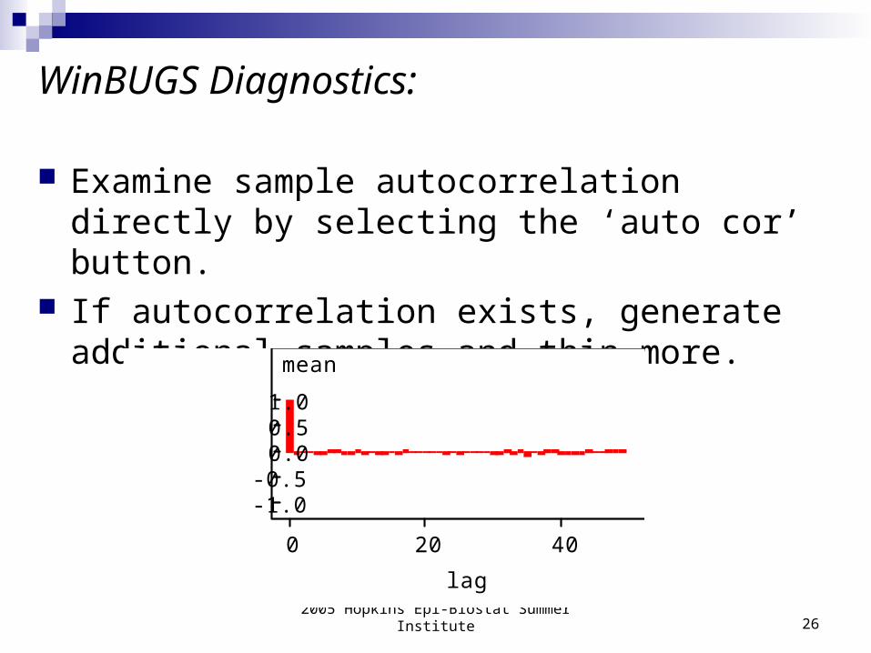
WinBUGS Diagnostics:
Examine sample autocorrelation directly by selecting the ‘auto cor’ button.
If autocorrelation exists, generate additional samples and thin more.
mean
lag
0 20 40
-1.0 -0.5 0.0 0.5 1.0
2005 Hopkins Epi-Biostat Summer Institute 27
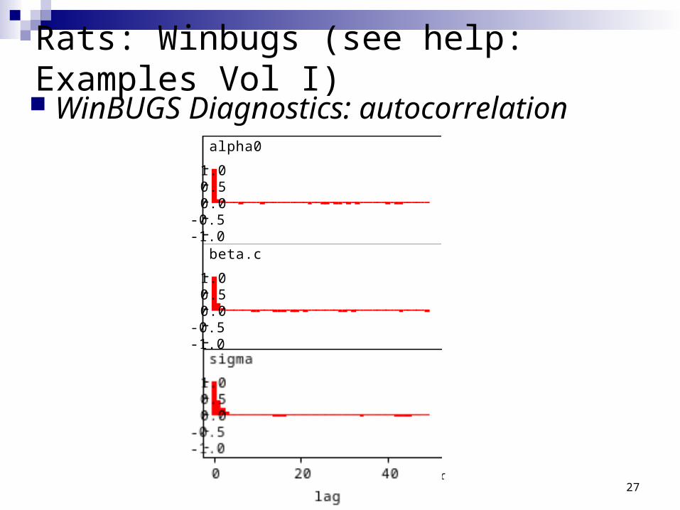
Rats: Winbugs (see help: Examples Vol I) WinBUGS Diagnostics: autocorrelation
alpha0
lag
0 20 40
-1.0 -0.5 0.0 0.5 1.0
beta.c
lag
0 20 40
-1.0 -0.5 0.0 0.5 1.0
2005 Hopkins Epi-Biostat Summer Institute 28
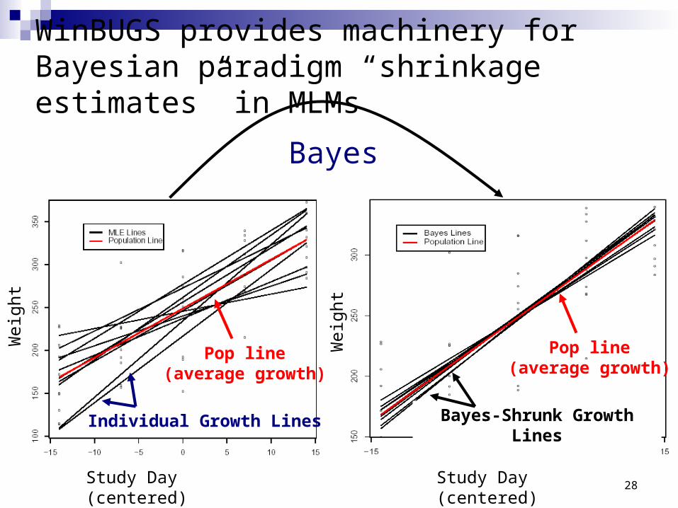
Bayes-Shrunk Growth Lines
WinBUGS provides machinery for Bayesian paradigm “shrinkage estimates” in MLMs
Pop line(average growth)
Wei
ght
Study Day (centered)
Pop line(average growth)
Study Day (centered)
Wei
ght
Individual Growth Lines
Bayes
2005 Hopkins Epi-Biostat Summer Institute 29
School Test Scores Revisited
2005 Hopkins Epi-Biostat Summer Institute 30
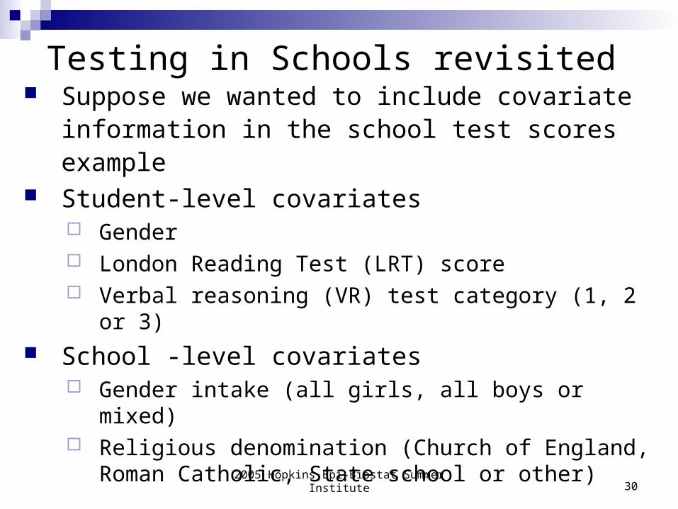
Testing in Schools revisited Suppose we wanted to include covariate
information in the school test scores example Student-level covariates
Gender London Reading Test (LRT) score Verbal reasoning (VR) test category (1, 2 or 3)
School -level covariates Gender intake (all girls, all boys or mixed) Religious denomination (Church of England,
Roman Catholic, State school or other)
2005 Hopkins Epi-Biostat Summer Institute 31
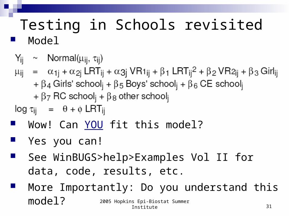
Testing in Schools revisited Model
Wow! Can YOU fit this model? Yes you can! See WinBUGS>help>Examples Vol II for data,
code, results, etc. More Importantly: Do you understand this model?
2005 Hopkins Epi-Biostat Summer Institute 32
Bayesian Concepts
Frequentist: Parameters are “the truth”
Bayesian: Parameters have a distribution
“Borrow Strength” from other observations
“Shrink Estimates” towards overall averages
Compromise between model & data
Incorporate prior/other information in estimates
Account for other sources of uncertainty
Posterior Likelihood * Prior


![2009 Convegno Malattie Rare Dominici [23 01]](https://img.pdfslide.net/doc/110x75/558e9a0c1a28ab8c708b4759/2009-convegno-malattie-rare-dominici-23-01.jpg)