2006-47(19) Polymer.pdf

7/27/2019 2006-47(19) Polymer.pdf

http://slidepdf.com/reader/full/2006-4719-polymerpdf 1/14

On the characterization of tensile creep resistance of polyamide 66nanocomposites. Part II: Modeling and prediction of long-term performance

Jing-Lei Yang a, Zhong Zhang b,*, Alois K. Schlarb a, Klaus Friedrich a

a Institute for Composite Materials, University of Kaiserslautern, 67663 Kaiserslautern, Germanyb National Center for Nanoscience and Technology, No. 2, 1st North Street Zhongguancun, 100080 Beijing, PR China

Received 10 January 2006; received in revised form 24 July 2006; accepted 24 July 2006

Abstract

The Part I of this study [Yang JL, Zhang Z, Schlarb AK, Friedrich K. Polymer 2006;47:2791e801] provided systematic experiments and

general discussions on the creep resistance of polyamide 66 nanocomposites. To promote these works, here we present some modeling and pre-

diction attempts in order to further understand the phenomena and mechanisms. Both a viscoelastic creep model named Burgers (or four-element

model) and an empirical method called Findley power law are applied. The simulating results from both models agree quite well with the

experimental data. An additional effort is conducted to understand the structureeproperty relationship based on the parameter analysis of

the Burgers model, since the variations in the simulating parameters illustrate the influence of nanofillers on the creep performance of the

bulk matrix. Moreover, the Eyring stress-activated process is taken into account by considering the activation volume. Furthermore, in order

to predict the long-term behavior based on the short-term experimental data, both the Burgers and Findley models as well as the timeetemper-

ature superposition principle (TTSP) were employed. The predicting capability of these modeling approaches is compared and the Findley power

law is preferred to be adopted. Master curves with extended time scale are constructed by applying TTSP to horizontally shift the short-time

experimental data. The predicting results confirm the enhanced creep resistance of nanofillers even at extended long time scale.

Ó 2006 Elsevier Ltd. All rights reserved.

Keywords: Creep modeling; Creep prediction; Polymer nanocomposites

1. Introduction

In view of the fact that nanomaterials as fillers become the

state-of-the-art in materials science, numerous studies have

been carried out and many improved mechanical properties

have been achieved with incorporations of nanofillers into

polymer matrices [1]. However, the complex performance of polymer nanocomposites can only be understood deeply by

combining experimental studies with effective modeling.

Therefore, modeling and simulation of polymer-based nano-

composites have become an essential issue due to the demand

for developing these materials to potential engineering appli-

cations. In the past years many modeling studies have been

carried out. Most of them have focused on the prediction of

elastic modulus, interfacial bonding or load transfer for either

carbon nanotubes [2e5] or spherical nanoparticles-filled

polymers [6e10].

Moreover, for the long period of loading, e.g., creep or

fatigue (must be taken into account in design, especially in

aviation and automotive applications [11,12]), it is usual thatthe material must remain in service for an extended period

of time, normally longer than it is practical to run creep exper-

iments on the materials to be employed. Therefore, it is neces-

sary to extrapolate the information obtained from relatively

short-term laboratory creep tests in order to predict the prob-

able behavior in service. However, to the best knowledge of

the authors, no analytical and prediction work has been

reported on the creep behavior of nanoparticle/thermoplastic

composites up to now. Recent work of Sarvestani and Picu

[13] proposed a network model to simulate the viscoelastic* Corresponding author.

E-mail address: [email protected] (Z. Zhang).

0032-3861/$ - see front matter Ó 2006 Elsevier Ltd. All rights reserved.

doi:10.1016/j.polymer.2006.07.060

Polymer 47 (2006) 6745e6758www.elsevier.com/locate/polymer

mailto:[email protected]

http://www.elsevier.com/locate/polymer

http://www.elsevier.com/locate/polymer

mailto:[email protected]

7/27/2019 2006-47(19) Polymer.pdf


behavior of nanoparticle/polymers. The rheology and shear

viscosity of nanocomposites were simulated by taking into ac-

count the important roles of the lifetime of the polymerefiller

junctions and the network of bridging segments. More recently

Blackwell and Mauritz [14] reported the shear creep behavior

of a sulfonated poly(styrene-b-ethylene/butylene-b-styrene)

(sSEBS)/silicate nanocomposite, the experimental data of

which could be satisfactorily simulated by using a modified

Burgers creep model. However, the shear creep experiments

were conducted by using a dynamic thermal analyzer

(DMA) within a very short time of 30 min and no further ex-

planations and discussions of the results were given. Although

the analytical work on the fluid viscoelasticity and the veryshort time creep of the nanocomposites presented some valu-

able points, some detailed explorations were needed for

practical applications.

In our previous experimental studies, the creep behavior of

a semicrystalline thermoplastic polyamide 66 (PA66) nano-

composites was systematically carried out at various tempera-

tures and different stress levels [1,15]. The creep deformation

and the creep rate of the matrix were reduced to different

extents by the addition of various nanofillers. Significantly

improved creep resistance broadens the research scope and, to-

gether with the enhanced crack initiation fracture toughness

[16,17], will certainly extend the potential applications of

nanocomposites. In addition, considering the design of nano-composites for engineering applications, modeling and pre-

dicting work becomes a key issue. Thus, in the present study

the modeling study based on experimental data by using tradi-

tional creep models [19,20] is conducted. An attempt to under-

stand the structureeproperty relationship is carried out based

on the parameter analysis of the Burgers model, since the var-

iations in the simulating parameters illustrate the influence of

nanofillers on the creep performance of the bulk matrix. More-

over, the Eyring stress-activated process [21] is taken into

account by considering the activation volume. Furthermore,

in order to predict the long-term behavior based on the

short-term experimental data, both the Burgers and Findleymodels as well as the timeetemperature superposition princi-

ple (TTSP) [21] were employed. Master curves with extended

time scale are constructed by applying TTSP to horizontally

shift the short-time experimental data. The predicting results

confirm the enhanced creep resistance of nanofillers even at

extended long time scale.

2. Theoretical background

2.1. Creep models

2.1.1. Burgers model

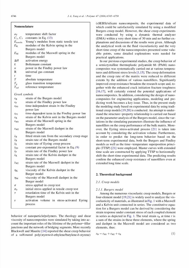
Among the numerous viscoelastic creep models, Burgers or

four-element model [19,21] is widely used to analyze the vis-

coelasticity of materials, as illustrated in Fig. 1 with a Maxwell

and a Kelvin unit connected in series. The constitutive equa-

tion for a Burgers model can be derived by considering the

strain response under constant stress of each coupled element

in series as depicted in Fig. 1. The total strain 3B at time t is

a sum of the strains in these three elements, where the spring

and dashpot in the Maxwell model are considered as two

elements, thus:

3B ¼ 3M1 þ 3M2 þ 3K ð1Þ

Nomenclature

aT temperature shift factor

C1, C2 constants in Eq. (13)

E tensile Young’s modulus from static tensile test

E K modulus of the Kelvin spring in theBurgers model

E M modulus of the Maxwell spring in the

Burgers model

D H activation energy

k Boltzmann constant

n power in the Findley power law

R universal gas constant

t time

T absolute temperature

T g glass transition temperature

T ref reference temperature

Greek symbols3B strain of the Burgers model

3F strain of the Findley power law

3F0 time-independent strain in the Findley

power law

3F1 time-dependent term in the Findley power law

3K strain of the Kelvin unit in the Burgers model

3M1 strain of the Maxwell spring in the

Burgers model

3M2 strain of the Maxwell dashpot in the

Burgers model

_3II fitted strain rate from the secondary creep stage

_3B strain rate of the Burgers model_3E strain rate of Eyring creep process

_3E0 constant pre-exponential factor in Eq. (9)

_3F strain rate of the Findley power law

_3K strain rate of the Kelvin dashpot in the

Burgers model

_3M2 strain rate of the Maxwell dashpot in the

Burgers model

hK viscosity of the Kelvin dashpot in the

Burger model

hM viscosity of the Maxwell dashpot in the

Burger model

s stress applied in creep test

s0 initial stress applied in tensile creep testt retardation time of the Kelvin unit in the

Burgers model

y activation volume in stress-activated Eyring

process

6746 J.-L. Yang et al. / Polymer 47 (2006) 6745e6758

7/27/2019 2006-47(19) Polymer.pdf


7/27/2019 2006-47(19) Polymer.pdf


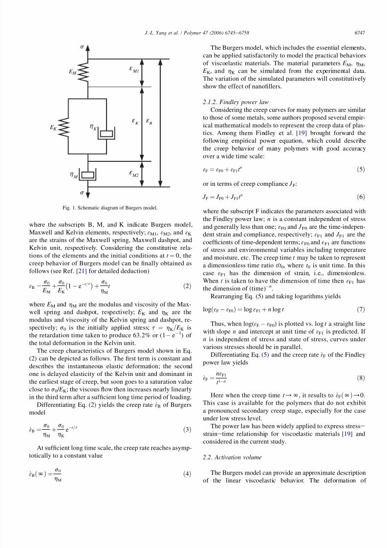
a polymer was also considered as an activated rate process

involving the motion of segments of chain molecules over po-tential barriers, and modified the standard linear solid so that

the movement of the dashpot was governed by the activated

process. As illustrated in Fig. 2, the Eyring model is intro-

duced here due to its useful parameter of activation volume

that may provide an indication of the underlying molecular

mechanisms. The activated rate process may also provide

a common basis for the discussion of creep behavior.

The creep rate of a stress-activated Eyring dashpot is given

by [21]:

_3E ¼ _3E0eÀD H kT sinh

ys

kT

ð9Þ

where the subscript E indicates an Eyring process; _3E0 is a con-

stant pre-exponential factor; D H represents the energy barrier

height; y is the activation volume for the molecular event; k , s

and T are Boltzmann constant, applied stress and absolute tem-

perature, respectively. Under high stress levels (s> 3kT / y) the

hyperbolic sine term can be approximated to ð1=2 expðys=kT ÞÞ .

Therefore, Eq. (9) can be simplified as:

_3E ¼1

2_3E0eÀððD H ÀysÞ=kT Þ ð10Þ

It follows that:

v ln _3E

vs¼

y

kT ð11Þ

Finally, approximate value of the activation volume for the

tested specimens can be obtained from the high stress levels,

e.g., in the current study s1¼ 30 MPa and s2¼ 40 MPa,

together with the corresponding steady creep rates under those

loads,

y¼ kT ðln _3EÞs2

Àðln _3EÞs1

s2 À s1

ð12Þ

The variation of the activation volume will show the effect

of nanofillers on the matrix.

2.3. Timeetemperature superposition principle (TTSP)

Many experiments of creep performance have been directed

at making long-term creep predictions from short-time creep

tests. The most acceptable methods for realizing this involve

using TTSP, which implies that the viscoelastic behavior at

one temperature can be related to that at another temperatureby a change in the time scale only. The detailed procedure is

that creep tests performed at high temperatures for short times

can mimic the creep behaviors performed at low temperatures

over long time scale [21,22].

In the current investigation, creep experiments of PA66 and

nanocomposites were carried out at three temperatures. The

creep data were then shifted horizontally along the logarithmic

time axis until they overlapped to form one continuous master

curve, which can be used to predict creep performance over

long time scale. If a reference temperature T ref other than

the glass transition temperature is selected, the shift factor

aT can be calculated by means of WLF Eq. [21]:

log aT ¼ÀC1

ÀT À T ref

ÁC2 þ

ÀT À T ref

Á ð13Þ

where C1 and C2 are constants dependent on the nature of the

material. Furthermore, the temperature dependent shift factor

aT is related to the activation energy D H as follows:

log aT ¼D H

2:303R

1

T À

1

T ref

ð14Þ

where R is the universal gas constant. The activation energy

can be obtained from the slope of the curve of log aT against

1/ T . The variation of D H shows the different effects of nano-

fillers on the matrix.

3. Materials and experimental procedure

As introduced in the Part I of this study [1], a widely

used polyamide 66 (PA66) was chosen as matrix. For nanofil-

lers, titanium dioxide particles with diameters of 300 nm and

21 nm were chosen. TiO2 particles (21 nm) treated with octyl-

silane to achieve a hydrophobic surface were considered as

well. Additionally, nanoclay was also selected. The volume

content of nanofillers was chosen as a constant of 1%. The

details and designations of the materials were given in Table 1

as well.

Uniaxial tensile creep experiments were preformed using

a Creep Rupture Test Machine with double lever system (Co-

esfeld GmbH, Model 2002). The elaborate experimental pro-

cedure was given in Part I [1] and the creep conditions were

listed in Table 1. The creep behavior of the materials was ob-

served within 200 h, which covered the primary and part of the

secondary creep stage. Modeling procedures were conducted

based on these experimental data.

P o t e n t i a l e n e r g y

H

Direction of flow and applied stress

Fig. 2. The Eyring model showing a stress activated process for creep.


7/27/2019 2006-47(19) Polymer.pdf


4. Modeling results and discussions

The experimental data were simulated by using the Non-

Linear Curve Fit function in OriginPro. The functions of the

Burgers model with four undetermined parameters and the

Findley power law with three undetermined parameters were

defined in OriginPro. The initial values of the parameters

were carefully chosen to make the calculation asymptotically

convergent to experimental data. Otherwise the bad initial

values led to non-convergent result and made the simulationfail. The simulation was performed by the program using

a least square approximation procedure and the parameters

were brought for further discussions.

4.1. Modeling parameters of Burgers model and

structuree property relationship

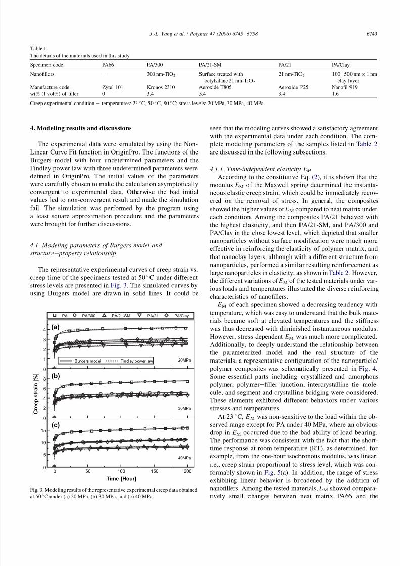
The representative experimental curves of creep strain vs.

creep time of the specimens tested at 50 C under different

stress levels are presented in Fig. 3. The simulated curves by

using Burgers model are drawn in solid lines. It could be

seen that the modeling curves showed a satisfactory agreement

with the experimental data under each condition. The com-

plete modeling parameters of the samples listed in Table 2

are discussed in the following subsections.

4.1.1. Time-independent elasticity E M

According to the constitutive Eq. (2), it is shown that the

modulus E M of the Maxwell spring determined the instanta-

neous elastic creep strain, which could be immediately recov-

ered on the removal of stress. In general, the compositesshowed the higher values of E M compared to neat matrix under

each condition. Among the composites PA/21 behaved with

the highest elasticity, and then PA/21-SM, and PA/300 and

PA/Clay in the close lowest level, which depicted that smaller

nanoparticles without surface modification were much more

effective in reinforcing the elasticity of polymer matrix, and

that nanoclay layers, although with a different structure from

nanoparticles, performed a similar resulting reinforcement as

large nanoparticles in elasticity, as shown in Table 2. However,

the different variations of E M of the tested materials under var-

ious loads and temperatures illustrated the diverse reinforcing

characteristics of nanofillers. E M of each specimen showed a decreasing tendency with

temperature, which was easy to understand that the bulk mate-

rials became soft at elevated temperatures and the stiffness

was thus decreased with diminished instantaneous modulus.

However, stress dependent E M was much more complicated.

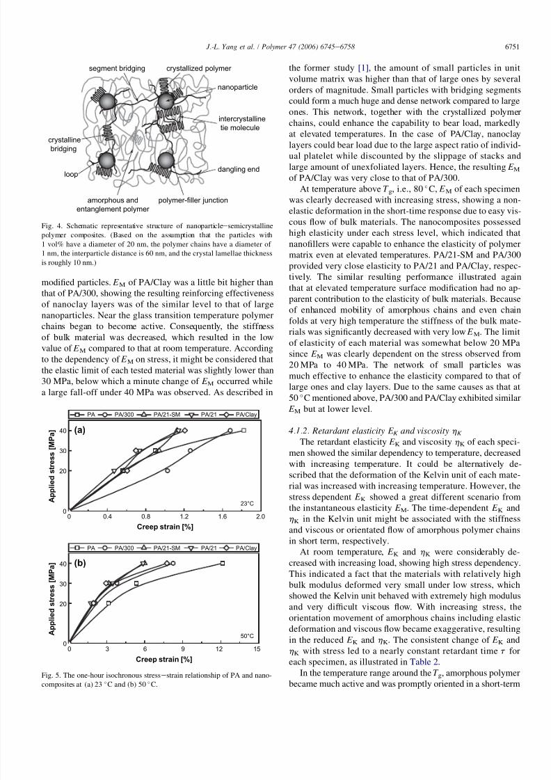
Additionally, to deeply understand the relationship between

the parameterized model and the real structure of the

materials, a representative configuration of the nanoparticle/

polymer composites was schematically presented in Fig. 4.

Some essential parts including crystallized and amorphous

polymer, polymerefiller junction, intercrystalline tie mole-

cule, and segment and crystalline bridging were considered.

These elements exhibited different behaviors under various

stresses and temperatures.

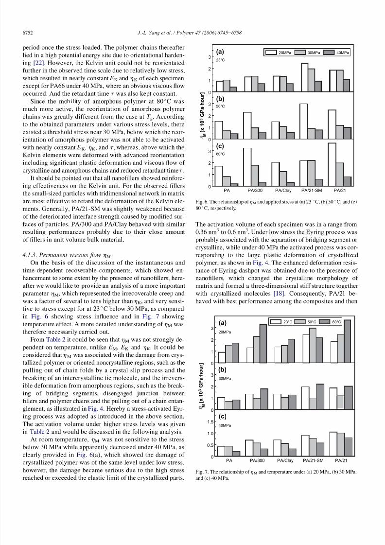
At 23 C, E M was non-sensitive to the load within the ob-

served range except for PA under 40 MPa, where an obvious

drop in E M occurred due to the bad ability of load bearing.

The performance was consistent with the fact that the short-

time response at room temperature (RT), as determined, for

example, from the one-hour isochronous modulus, was linear,

i.e., creep strain proportional to stress level, which was con-

formably shown in Fig. 5(a). In addition, the range of stress

exhibiting linear behavior is broadened by the addition of

nanofillers. Among the tested materials, E M showed compara-

tively small changes between neat matrix PA66 and the

Table 1

The details of the materials used in this study

Specimen code PA66 PA/300 PA/21-SM PA/21 PA/Clay

Nanofillers e 300 nm-TiO2 Surface treated with

octylsilane 21 nm-TiO2

21 nm-TiO2 100e500 nmÂ 1 nm

clay layer

Manufacture code Zytel 101 Kronos 2310 Aeroxide T805 Aeroxide P25 Nanofil 919

wt% (1 vol%) of filler 0 3.4 3.4 3.4 1.6

Creep experimental condition e temperatures: 23 C, 50 C, 80 C; stress levels: 20 MPa, 30 MPa, 40 MPa.

0

1

2

3

4

PA PA/300 PA/21-SM PA/21 PA/Clay

C r e e p s

t r a i n [ % ]

Burgers model Findley power law

0

2

4

6

8

30MPa

0

5

10

15

Time [Hour]

40MPa

20MPa

(a)

(b)

(c)

0 50 100 150 200

Fig. 3. Modeling results of the representative experimental creep data obtained

at 50 C under (a) 20 MPa, (b) 30 MPa, and (c) 40 MPa.


7/27/2019 2006-47(19) Polymer.pdf


nanocomposites, which provided the fact that the instanta-

neous elasticity was not much altered by the addition of nano-

fillers. The instantaneous elasticity E M was reasonably

corresponding to the elasticity of the crystallized polymer or

regular chain folds, which took the immediate load due to

high stiffness compared to amorphous polymers, as illustrated

in Fig. 4. However, although the crystalline morphology was

changed by the addition of nanofillers the crystallinity of

each specimen was not obviously altered [17,18], which im-

plied the load bearing parts were not of great difference

between neat matrix and nanocomposites.

At 50 C, with increasing stress levels E M of each specimen

was decreased slightly from 20 MPa to 30 MPa and

significantly reduced under high stress of 40 MPa. It was

reasonable to believe that there existed a threshold of linear

viscoelasticity near the stress of 30 MPa in the short-time re-

sponse, which was also consistent with the one-hour isochro-

nous stressestrain relationship in Fig. 5(b). Among the

observed specimens, the nanocomposites behaved with much

better elasticity compared to pure matrix, showing an effective

reinforcement by the addition of nanofillers near the glass

transition temperature. E M was increased with decreasing par-

ticle size under each stress level while the value of PA/21-SM

was very close to that of PA/21, depicting at 50 C nanopar-

ticles with surface modification had no obvious contribution

to the elasticity of the bulk material compared to non-surface

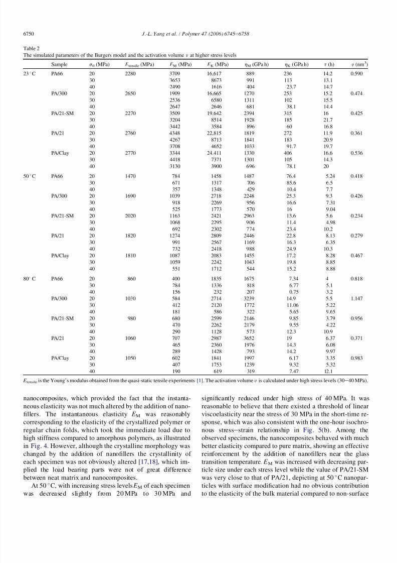
Table 2

The simulated parameters of the Burgers model and the activation volume y at higher stress levels

Sample s0 (MPa) E tensile (MPa) E M (MPa) E K (MPa) hM (GPa h) hK (GPa h) t (h) y (nm3)

23 C PA66 20 2280 3709 16,617 889 236 14.2 0.590

30 3653 8673 991 113 13.1

40 2490 1616 404 23.7 14.7

PA/300 20 2650 1909 16,665 1270 253 15.2 0.474

30 2536 6580 1311 102 15.540 2647 2646 681 38.1 14.4

PA/21-SM 20 2270 3509 19,642 2394 315 16 0.425

30 3204 8514 1928 185 21.7

40 3442 3584 896 60 16.8

PA/21 20 2760 4348 22,815 1819 272 11.9 0.361

30 4267 8713 1841 183 20.9

40 3708 4652 1033 91.7 19.7

PA/Clay 20 2770 3344 24,411 1330 406 16.6 0.536

30 4418 7371 1301 105 14.3

40 3130 3900 696 78.1 20

50 C PA66 20 1470 784 1458 1487 76.4 5.24 0.418

30 671 1317 706 85.6 6.5

40 357 1348 429 10.4 7.7

PA/300 20 1690 1039 2718 2248 25.3 9.3 0.42630 918 2269 956 16.6 7.31

40 525 1773 570 16 9.04

PA/21-SM 20 2020 1163 2421 2963 13.6 5.6 0.234

30 1068 2295 906 11.4 4.98

40 692 2302 774 23.4 10.2

PA/21 20 1820 1274 2809 2446 22.8 8.13 0.279

30 991 2567 1169 16.3 6.35

40 732 2418 988 24.9 10.3

PA/Clay 20 1810 1087 2083 1455 17.2 8.28 0.467

30 1059 2242 1043 19.8 8.85

40 551 1712 544 15.2 8.88

80 C PA66 20 860 400 1835 1675 7.34 4 0.818

30 284 1336 818 6.77 5.1

40 156 232 207 0.75 3.2

PA/300 20 1030 584 2714 3239 14.9 5.5 1.147

30 412 2120 1772 11.06 5.22

40 181 586 322 5.65 9.65

PA/21-SM 20 980 680 2599 2146 9.85 3.79 0.956

30 470 2262 2179 9.55 4.22

40 290 1128 573 12.3 10.9

PA/21 20 1060 707 2987 3652 19 6.37 0.371

30 465 2360 1976 14.3 6.08

40 289 1428 793 14.2 9.97

PA/Clay 20 1050 602 1841 1997 6.17 3.35 0.983

30 407 1753 1239 9.32 5.32

40 190 619 319 7.47 12.1

E tensile is the Young’s modulus obtained from the quasi-static tensile experiments [1]. The activation volume y is calculated under high stress levels (30e40 MPa).


7/27/2019 2006-47(19) Polymer.pdf


modified particles. E M of PA/Clay was a little bit higher than

that of PA/300, showing the resulting reinforcing effectiveness

of nanoclay layers was of the similar level to that of large

nanoparticles. Near the glass transition temperature polymer

chains began to become active. Consequently, the stiffness

of bulk material was decreased, which resulted in the low

value of E M compared to that at room temperature. According

to the dependency of E M on stress, it might be considered that

the elastic limit of each tested material was slightly lower than

30 MPa, below which a minute change of E M occurred while

a large fall-off under 40 MPa was observed. As described in

the former study [1], the amount of small particles in unit

volume matrix was higher than that of large ones by several

orders of magnitude. Small particles with bridging segments

could form a much huge and dense network compared to large

ones. This network, together with the crystallized polymer

chains, could enhance the capability to bear load, markedly

at elevated temperatures. In the case of PA/Clay, nanoclaylayers could bear load due to the large aspect ratio of individ-

ual platelet while discounted by the slippage of stacks and

large amount of unexfoliated layers. Hence, the resulting E Mof PA/Clay was very close to that of PA/300.

At temperature above T g, i.e., 80 C, E M of each specimen

was clearly decreased with increasing stress, showing a non-

elastic deformation in the short-time response due to easy vis-

cous flow of bulk materials. The nanocomposites possessed

high elasticity under each stress level, which indicated that

nanofillers were capable to enhance the elasticity of polymer

matrix even at elevated temperatures. PA/21-SM and PA/300

provided very close elasticity to PA/21 and PA/Clay, respec-

tively. The similar resulting performance illustrated againthat at elevated temperature surface modification had no ap-

parent contribution to the elasticity of bulk materials. Because

of enhanced mobility of amorphous chains and even chain

folds at very high temperature the stiffness of the bulk mate-

rials was significantly decreased with very low E M. The limit

of elasticity of each material was somewhat below 20 MPa

since E M was clearly dependent on the stress observed from

20 MPa to 40 MPa. The network of small particles was

much effective to enhance the elasticity compared to that of

large ones and clay layers. Due to the same causes as that at

50 C mentioned above, PA/300 and PA/Clay exhibited similar

E M but at lower level.

4.1.2. Retardant elasticity E K and viscosity h K

The retardant elasticity E K and viscosity hK of each speci-

men showed the similar dependency to temperature, decreased

with increasing temperature. It could be alternatively de-

scribed that the deformation of the Kelvin unit of each mate-

rial was increased with increasing temperature. However, the

stress dependent E K showed a great different scenario from

the instantaneous elasticity E M. The time-dependent E K and

hK in the Kelvin unit might be associated with the stiffness

and viscous or orientated flow of amorphous polymer chains

in short term, respectively.

At room temperature, E K and hK were considerably de-

creased with increasing load, showing high stress dependency.

This indicated a fact that the materials with relatively high

bulk modulus deformed very small under low stress, which

showed the Kelvin unit behaved with extremely high modulus

and very difficult viscous flow. With increasing stress, the

orientation movement of amorphous chains including elastic

deformation and viscous flow became exaggerative, resulting

in the reduced E K and hK . The consistent change of E K and

hK with stress led to a nearly constant retardant time t for

each specimen, as illustrated in Table 2.

In the temperature range around the T g, amorphous polymer

became much active and was promptly oriented in a short-term

crystallized polymer

amorphous and

entanglement polymer

nanoparticle

segment bridging

crystalline

bridging

dangling end

polymer-filler junction

intercrystalline

tie molecule

loop

Fig. 4. Schematic representative structure of nanoparticleesemicrystalline

polymer composites. (Based on the assumption that the particles with

1 vol% have a diameter of 20 nm, the polymer chains have a diameter of

1 nm, the interparticle distance is 60 nm, and the crystal lamellae thickness

is roughly 10 nm.)

0 0.4 0.8 1.2 1.6 2.00

20

30

40

A p p l i e d s t r e s s [ M P a ]



Creep strain [%]

0 3 6 9 12 150

20

30

40

A p p l i e d s t r e s s [ M P a ]

Creep strain [%]

23°C

50°C

(b)

(a)

Fig. 5. The one-hour isochronous stressestrain relationship of PA and nano-

composites at (a) 23 C and (b) 50 C.


7/27/2019 2006-47(19) Polymer.pdf


period once the stress loaded. The polymer chains thereafter

lied in a high potential energy site due to orientational harden-

ing [22]. However, the Kelvin unit could not be reorientated

further in the observed time scale due to relatively low stress,

which resulted in nearly constant E K and hK of each specimen

except for PA66 under 40 MPa, where an obvious viscous flow

occurred. And the retardant time t was also kept constant.Since the mobility of amorphous polymer at 80 C was

much more active, the reorientation of amorphous polymer

chains was greatly different from the case at T g. According

to the obtained parameters under various stress levels, there

existed a threshold stress near 30 MPa, below which the reor-

ientation of amorphous polymer was not able to be activated

with nearly constant E K , hK , and t, whereas, above which the

Kelvin elements were deformed with advanced reorientation

including significant plastic deformation and viscous flow of

crystalline and amorphous chains and reduced retardant time t.

It should be pointed out that all nanofillers showed reinforc-

ing effectiveness on the Kelvin unit. For the observed fillers

the small-sized particles with tridimensional network in matrixare most effective to retard the deformation of the Kelvin ele-

ments. Generally, PA/21-SM was slightly weakened because

of the deteriorated interface strength caused by modified sur-

faces of particles. PA/300 and PA/Clay behaved with similar

resulting performances probably due to their close amount

of fillers in unit volume bulk material.

4.1.3. Permanent viscous flow h M

On the basis of the discussion of the instantaneous and

time-dependent recoverable components, which showed en-

hancement to some extent by the presence of nanofillers, here-

after we would like to provide an analysis of a more importantparameter hM, which represented the irrecoverable creep and

was a factor of several to tens higher than hK , and very sensi-

tive to stress except for at 23 C below 30 MPa, as compared

in Fig. 6 showing stress influence and in Fig. 7 showing

temperature effect. A more detailed understanding of hM was

therefore necessarily carried out.

From Table 2 it could be seen that hM was not strongly de-

pendent on temperature, unlike E M, E K and hK . It could be

considered that hM was associated with the damage from crys-

tallized polymer or oriented noncrystalline regions, such as the

pulling out of chain folds by a crystal slip process and the

breaking of an intercrystalline tie molecule, and the irrevers-

ible deformation from amorphous regions, such as the break-

ing of bridging segments, disengaged junction between

fillers and polymer chains and the pulling out of a chain entan-

glement, as illustrated in Fig. 4. Hereby a stress-activated Eyr-

ing process was adopted as introduced in the above section.

The activation volume under higher stress levels was given

in Table 2 and would be discussed in the following analysis.

At room temperature, hM was not sensitive to the stress

below 30 MPa while apparently decreased under 40 MPa, as

clearly provided in Fig. 6(a), which showed the damage of

crystallized polymer was of the same level under low stress,

however, the damage became serious due to the high stress

reached or exceeded the elastic limit of the crystallized parts.

The activation volume of each specimen was in a range from

0.36 nm3 to 0.6 nm3. Under low stress the Eyring process was

probably associated with the separation of bridging segment or

crystalline, while under 40 MPa the activated process was cor-

responding to the large plastic deformation of crystallized

polymer, as shown in Fig. 4. The enhanced deformation resis-

tance of Eyring dashpot was obtained due to the presence of

nanofillers, which changed the crystalline morphology of

matrix and formed a three-dimensional stiff structure togetherwith crystallized molecules [18]. Consequently, PA/21 be-

haved with best performance among the composites and then

0

1

2

320MPa 30MPa 40MPa

23°C

50°C

80°C

0

1

2

3

PA PA/300 PA/Clay PA/21-SM PA/21

0

1

2

3

(a)

(b)

(c)

M

[ x 1 0 3 G

P a · h o u r

]

Fig. 6. The relationship of hM and applied stress at (a) 23 C, (b) 50 C, and (c)

80 C, respectively.

0

1

2

3

0

1

2

3

PA PA/300 PA/Clay PA/21-SM PA/210

0.5

1.0

1.5

20MPa

30MPa

40MPa

(a)

(b)

(c)

M

[ x 1 0 3 G

P

a · h o u r ]

23°C 50°C 80°C

Fig. 7. The relationship of hM and temperature under (a) 20 MPa, (b) 30 MPa,

and (c) 40 MPa.


7/27/2019 2006-47(19) Polymer.pdf


PA/21-SM. Large particles and nanoclay layers exhibited sim-

ilar resulting performance.

In the case of 50 C, hM was significantly decreased with

increasing stress, reflecting the fact of increment of irrecover-

able deformation, as shown in Fig. 6(b). The activation volume

of each specimen was smaller than that at 23 C, indicating

a much local molecular process near T g, such as the breakingof an intercrystalline tie molecule and detaching of polymere

filler junction, as illustrated in Fig. 4. The irreversible creep

strain was diminished by the addition of nanofillers, which en-

hanced the immobility of polymer chains and resulted in

a much local Eyring process in the meantime. PA/21 behaved

with the least permanent deformation while PA/21-SM showed

the smallest activation volume due to a uniform dispersion of

particles with surface modification. Nanoclay layers had no

obvious advantage over large nanoparticles on affecting the

molecular process.

A similar scenario occurring at 80 C compared to that at

50 C that hM was considerably decreased with increasing

stress, is shown in Fig. 6(c). However, an interesting phenome-non was presented that the activation volume of each specimen

was the largest among the observed temperatures, probably in-

dicating a different stress-activated process at 80 C. Polymer

chains were highly thermally activated at this temperature.

Large deformation of crystallized polymer such as the pulling

out of chain folds by a crystal slip process and the irreversible

transition of amorphous polymer such as the pulling out of

chain entanglement and orientation crystallization under exter-

nal stress [18,24], were relatively large scale cooperation of de-

formation. While the stress-activated process could partially be

resisted by the appearance of nanofillers, which acted as block-

ing sites to retard or restrict the slippage of crystallized polymerby reducing the size of crystal part and disentanglement of

amorphous chains. Among the observed fillers, small particles

without surface modification possessed the most applicability

and resulted in the smallest activation volume. However, other

composites behaved with better hM while larger activation vol-

ume than neat matrix, which indicated that the mobility of these

fillers in matrix became active compared to that of small parti-

cles without surface modification.

hM showed a clear dependence on stress and was explained

by using Eyring stress-activated process. Although hM was not

sensitive to temperature, there were, however, some interesting

trends under each stress level, as shown in Fig. 7. In general,

hM was increased with increasing temperature under 20 MPa

except for PA/21-SM, in which hM was decreased at 80 C,

as illustrated in Fig. 7(a). The result indicates a fact that under

low stress levels the permanent deformation of each specimen

was reduced at elevated temperatures, which may be due to

that small load could not activate many polymer segments or

damage polymer structure permanently at high temperatures.

Accordingly, the bulk materials were highly thermally acti-

vated other than stress activated at elevated temperatures and

thus behaved with strong recoverable capability, which con-

firmed with decreased retardant time under 20 MPa, as shown

in Table 2. However, under higher stress level, e.g., 40 MPa,

advanced creep processes were stress activated, such as the

slippage of crystallized polymer and the disentanglement of

amorphous polymer, in a large scale of mobility with great ir-

reversible deformation and large activation volume, as shown

in Fig. 7(c) and Table 2, respectively. It was noteworthy to

point out that in the case of 30 MPa hM showed an ambiguous

dependence on temperature. hM at 80 C was slightly changed

compared to that at 23

C for each specimen, however, obvi-ously decreased to a very close value for all observed materials

at 50 C, as shown in Fig. 7(b). At 23 C, since the materials

were not thermally activated and the moderately low external

stress was not able to make a pronounced creep process, the vis-

cous flow was not obviously activated and was in relatively low

level. However, at 80 C, large instantaneous deformation re-

sulted due to many thermally activated polymer chains under

external stress. Therefore, the orientation of polymer chains oc-

curred to a great extent and resulted in highly orientating hard-

ening and crystallization in bulk materials [18,23]. Thereafter

the advanced creep flow became much difficult and the resulting

hM at 80 C was very close to that at 23 C. It was a different

scene at 50 C, at which materials began to enter the glass tran-sition region and the amount of thermally activated chains was

small. What was most important was the degree of the instanta-

neous deformation and orientation, which was very mild and led

to low orientation hardening compared to that at 80 C. It indi-

cated the materials had the potential to perform advanced vis-

cous flow with increasing time under this condition. This was

confirmed by the directly fitted creep rates [1], which were

dominated by hM at large time scale according to Eq. (3).

4.2. Modeling parameters from Findley power law

The Burgers model provided a constitutive representativeand the modeling parameters showed a detailed structure-to-

property relationship of the polymer composites. Additionally,

an empirical model, i.e., Findley power law, was frequently

applied to simulate and predict the long-term creep properties

due to its simple expression and satisfactory applicability [19].

Hereby this method was also adopted to provide a wide under-

standing of the creep performance of nanocomposites.

The simulated sample curves of specimens at 50 C were

illustrated as dash lines in Fig. 3 under 20 MPa (a), 30 MPa

(b), and 40 MPa (c). It could be seen that the fitting curves

agreed very well with the experimental data. Since the power

n of each specimen was not sensitive to stress, it was consid-

ered as constant at each temperature. The complete modeling

parameters 3F0, 3F1 and n under each condition are listed in

Table 3, from which an explicit dependency both on stress

and on temperature of the modeling parameters came into

view. On the one hand, both the time-independent strain 3F0

and time-dependent term 3F1 showed obvious growth with in-

creasing stress level at each temperature; on the other hand, it

exhibited the same behavior that 3F0 and 3F1 were increased

with increasing temperature under each stress level. However,

the increasing amplitude of 3F1 was quickly slowed down from

50 C to 80 C under stress below 30 MPa, which showed that

3F1 was not sensitive to temperature under moderately low

stress level. The behavior of 3F0 was equivalent to the


7/27/2019 2006-47(19) Polymer.pdf


instantaneous deformation 3M1 of Burgers model in nature,

where the representative parameter was the elasticity E M of

the Maxwell spring. Additionally, the increment of 3F0 and

3F1 dependent on whatever temperature or stress were signifi-

cantly reduced by the addition of nanofillers. In particular, PA/

21 behaved with the minimum 3F0 and 3F1, and then PA/21-

SM. PA/300 and PA/Clay were on the same level with slight

enhancement compared to that of matrix PA66. The feature

of 3F0 was also coincident with that of E M as discussed above.

In addition, according to Eq. (7), the fitting curves of

log strain difference (creep strain 3FÀ instantaneous strain

3F0) vs. log time t for PA and PA/21 under various stress levelsare provided in Fig. 8 at 23 C (a), 50 C (b), and 80 C (c). It

could be seen that the fitting curves of each specimen were

parallel and agreed very well with the experimental data, espe-

cially over large time scale, which indicated that the power n

was independent of stress and state of stress. From the figures

it could also be obtained that the power n of PA/21 was almost

the same as that of PA66 at 23 C while slightly higher than

that of PA66 at elevated temperatures. This phenomenon im-

plied that the nanofillers applied in this study could not affect

the parameter n so much, as shown in Table 3.

It could also be found from the curves in Fig. 8 that in the

first several hours the fitting lines, however, were not coincid-

ing well with the experimental data. This case might be due tothe restriction of the loading system of the creep machine, by

which the specimen was loaded to reach up to the desired

stress asymptotically after sometime [25] and the experimental

creep strain in the beginning stage was smaller than the real

one. The numbers on the left in Fig. 8 indicated the strain at

1 h. To determine the strain represented by the curves, shift

vertical scale to match this number.

4.3. Creep rates

Both the constitutive Burgers model and empirical Findley

power law could be fitted to the experimental strain very well.

In addition, another important parameter, creep rate, was also

necessary to describe the creep characteristics. The complete

creep rates at creep time equal to 200 h obtained from Burgers

model ð_3BÞ and Findley power law ð_3FÞ were listed in Table 4

for each specimen. Comparatively, the directly fitting creep

rates ð_3IIÞ from the secondary creep stage were provided there

as well. It could be found from the table that _3B and _3F were

very close to _3II and showed the same dependency on both

temperature and stress as _3II, which was already discussed in

the Part I of the study [1].

However, the detailed creep rate values of these two models

indicated their intrinsic characteristics. In general,_3F was lessthan _3B for each specimen under each condition. At room tem-

perature, both _3B and _3F were slightly lower than _3II, showing

the same applicability of the two models at ambient tempera-

ture. At the elevated temperatures, _3B was gently larger than _3II

while _3F fairly lower than _3II for each specimen. This case

hinted that the Burgers model was capable and precise enough

to characterize the experimental data of nanocomposites,

whereas the Findley power law was applicable to describe

the creep behaviors that did not exhibit a pronounced second-

ary stage, especially over large time scale at temperatures

above T g. Their intrinsic difference could result in distinct ca-

pability to predict the long-term performance via short-term

experiments, which would be discussed in the followingsection.

5. Prediction of long-term properties of nanocomposites

5.1. Prediction by both models

Both Burgers model and Findley power law are very widely

applied to describe the creep behaviors of a number of differ-

ent plastics, laminated plastics, wood, concrete and some

metals as well [19]. Thereafter as an example we provided

the prediction of creep strains of PA66, PA/300, and PA/21.

Data for these experiments and constants corresponding to

Table 3

The simulated parameters of the Findley power law

Sample s0 (MPa) 23 C 50 C 80 C

3F0 (%) 3F1 (10À4 h1/ n) n 3F0 (%) 3F1 (10À4 h1/ n) n 3F0 (%) 3F1 (10À4 h1/ n) n

PA66 20 0.312 15.0 0.296 1.826 143 0.0978 3.942 169 0.0658

30 0.601 22.7 2.249 317 7.259 442

40 1.109 102.1 6.222 573 12.78 2380PA/300 20 0.862 13.3 0.276 1.360 84.5 0.108 2.955 86.7 0.0848

30 0.994 24.8 1.834 188.4 6.159 185

40 1.105 71.0 4.173 394 11.30 1280

PA/21-SM 20 0.488 7.2 0.288 1.426 72.5 0.108 2.546 84.7 0.0896

30 0.761 18.0 1.678 171 5.768 139

40 0.821 50.7 3.044 307 7.962 671

PA/21 20 0.349 8.9 0.276 1.038 82.6 0.103 2.078 109 0.0663

30 0.498 19.9 1.921 159 4.756 231

40 0.610 48.2 3.034 281 7.415 722

PA/Clay 20 0.446 9.8 0.302 1.122 109 0.111 3.175 87.2 0.0951

30 0.566 18.9 1.422 184 6.112 209

40 0.695 54.6 3.822 395 10.81 1160


7/27/2019 2006-47(19) Polymer.pdf


Table 4

Comparison of the creep rates obtained from different models and direct linear regression

Sample s0 (MPa) 23 C (10À6 /h) 50 C (10À6 /h) 80 C (10À6 /h)

_3B _3F _3II _3B _3F _3II _3B _3F _3II

PA66 20 22.5 10.7 22.6 13.4 11.7 8.01 11.9 7.88 4.79

30 30.3 16.1 24.3 42.5 26.0 34.6 36.7 20.6 26.6

40 99.0 72.5 103 93.2 47.0 88.3 193 111 137

PA/300 20 15.7 7.92 16.4 8.90 8.09 8.06 6.17 5.76 1.6830 22.9 14.8 19.1 31.4 18.0 26.3 16.9 12.3 10.6

40 58.7 42.3 61.2 70.2 37.7 68.3 124 85.1 111

PA/21-SM 20 8.35 4.77 8.63 6.75 6.94 4.36 9.32 6.10 2.35

30 15.6 11.9 16.7 33.1 16.4 30.0 13.8 10.0 9.25

40 44.6 33.6 47.4 51.7 29.4 50.7 69.8 48.3 65.8

PA/21 20 11.0 5.30 11 8.18 7.34 6.84 5.48 5.13 1.68

30 16.3 11.9 17.7 25.7 14.1 21.3 15.2 10.9 21.3

40 38.7 28.7 42.9 40.5 25.0 39.8 50.4 34.0 45.6

PA/Clay 20 15.0 7.33 15.2 13.7 10.9 12.1 10.0 6.86 11.2

30 23.0 14.1 17.1 28.8 18.4 25.6 24.2 16.4 16.3

40 57.5 40.8 63.7 73.5 39.5 73.0 125 91.3 122

The creep rates _3B and _3F are calculated by using Findley power law and Burgers model, respectively, at time t ¼ 200 h. _3II is directly fitted from the secondary

creep stage in the creep strain vs. time curve [1].

0.1 1 10 100

101

100

10-1

101

100

10-110-2

PA

PA/21

simulated results

1.21

0.74

0.47

2.06

0.92

Time [hour]

0.57

23°C

0.1 1 10 100

PA

PA/21

simulated results

50°C

Time [hour]

5.85

3.30

1.77

11.2

5.49

3.17

20MPa 30MPa 40MPa20MPa 30MPa 40MPa

(a) (b)

102

100

101

10-1

0.1 1 10 100

20MPa 30MPa 40MPa

PA

PA/21

simulated results

80°C

Time [hour]

14.2

6.93

3.08

32.3

10.8

5.22

(c)

Fig. 8. Log strain difference 3FÀ 3F0 vs. log time t for PA and PA/21 at (a) 23 C, (b) 50 C, and (c) 80 C. (Note: numbers on left indicate strain at 1 h.

To determine strain, shift vertical scale to match this number.)


7/27/2019 2006-47(19) Polymer.pdf


Eqs. (2) and (5) were determined from the first 100 h creep.

The tests, however, were continued uninterrupted for roughly

360 h. Subsequently, these data were compared with predic-

tions from Eqs. (2) and (5) based on the constants previously

determined. The results were shown in Fig. 9. Although the

modeling curves agreed very well with the experimental

data within the applied time period, i.e., 100 h, it could obvi-ously be seen over that period the prediction of the Findley

power law was very satisfactory and that of the Burgers model,

however, showed a huge deviation from the experimental data.

Hence, the accuracy with which a creep equation describes the

time dependence becomes an important consideration. There-

fore, it is necessary and useful to analyze the difference

between the creep models applied in this study in order to

obtain a deep understanding in nature.

According to the above simulation results, these two

models could describe the creep behavior satisfactorily in

terms of both creep strain and creep rate within the experimen-

tal time range. Additionally, considering Eq. (3), the creep rate

of the Burgers model was dominant with hM and hK , while the

contribution of the latter was greatly controlled by the value of

eÀt =t. When the creep time was relatively long, e.g., 100 h in

the current study, t was calculated less than 10 h at 80 C.

Thus, eÀt =t was about 10À5 and Eq. (3) could be approximated

to Eq. (4), which indicated the creep rate was thereafter con-

stant and totally controlled by the permanent viscous flowhM. However, the inner structures of the materials became

much complicated due to the cooperative influences of stress

and elevated temperature with increasing time, which implied

that hM was highly time-dependent and couldnot be used to rep-

resent the future behavior. Comparatively, the creep rate equa-

tion deduced with time from the Findley power law might

imply a true case that the thermoplastic nanocomposites be-

haved with a non-pronounced secondary creep stage and there-

fore it was satisfactory to predict the creep characteristics over

a large time scale [18,19].

As an example, the Findley power law was applied to pre-

dict the long-term creep behavior of PA and nanocomposites.

The prediction was executed up to 2000 h based on the 250-hexperimental data, as shown in Fig. 9(b). It confirms that the

power law displays very good predicting performance, which

is widely applied in engineering applications [19]. From the

predicted curves, it was found that the creep resistance of

nanocomposites was also obviously enhanced compared to

that of neat matrix even at long-term scale, which confirms

with the short-term experiments.

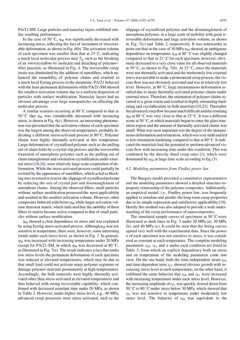
5.2. Prediction by the timeetemperature superposition

method

The analysis in the former subsection confirmed that theFindley power law was a satisfactory means to predict the

long-term creep performance. Furthermore, we would like to

provide another method, i.e., timeetemperature superposition

principle, to observe the long-term property of nanocompo-

sites. The creep strains were measured at 23, 40, and 50 C,

respectively, under a constant load of 15 MPa for appropriate

time scale to make sure of the strain overlap at neighboring

temperatures. The sample curves of PA66 and PA/21 were pre-

sented as creep compliance in Fig. 10(a). It could also be seen

that both the creep compliance and creep rate were signifi-

cantly reduced in PA/21 at each temperature. The sample mas-

ter creep compliance curves of three materials were illustrated

in Fig. 10(b). The master curves were extended up to 1010 s in

time scale. The creep compliance of PA/21 was obviously

lower than that of PA, which showed the reinforcing effective-

ness of nanoparticles. The increment of compliance with time

was slowed down from 109 to 1010 s, showing the materials

entered into a rubbery state [21] over an extremely long period

of time. The viscoelastic stage data were simulated by using

Eq. (6) and the resulting curves satisfactorily agreed with

the master creep data. The reduced parameters were obtained

and given in Table 5.

The shift factor showed a good linear dependence on the

temperature, as given in Fig. 10(b) with insertion graph. The

activation energy was obtained by the slope of a plot of log aT

200 3000 100 4000

4

8

12

16

PA PA/300 PA/21

Burgers Findley

C r e e p s t r a i n [ % ]

Creep time [hour]

Creep time [hour]

30MPa/80°C

0 500 1000 1500 20000

1

2

3

4

5

20MPa/50°C

C r e e p s t r a i n [ % ]

PA66 PA/300 PA/Clay

PA/21-SM PA/21 Findley

(a)

(b)

Fig. 9. Prediction by using creep models: (a) comparison of the predicting abil-

ity of the Burgers model and Findley power law for PA and the nanocompo-

sites under 30 MPa/80 C; (b) the application of Findley power law to predict

the creep deformation of PA and the nanocomposites under 20 MPa/50 C in

2000 h based on the 250 h experimental data.


7/27/2019 2006-47(19) Polymer.pdf


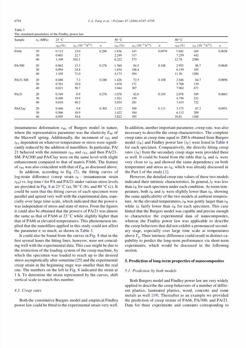
against 1/ T , as expressed in Eq. (14). The calculated values are

listed in Table 5. The activation energy of the nanocomposites

except for PA/21 was higher than that of PA66, which, to-

gether with the reduced activation volume at 50 C obtained

in Table 2, indicated that the immobilization of polymer

chains became much difficult due to the addition of nanofil-

lers. However, in the case of PA/21 although the activation en-

ergy was very close to that of matrix, the small nanoparticles

still exhibited the reinforcing effect because a considerable re-

duction of the activation volume had resulted due to their

presence.

6. Conclusions

In the current study the modeling of creep deformation of

PA66 and its nanocomposites were satisfactorily conducted

by using Burgers model and Findley power law. The simulat-

ing parameters helped to comprehensively understand the

creep resistant composites by the addition of nanofillers and

suggested the structureeproperty relationship representatively.

Additionally, the long-term behavior was predicted by using

the Findley model and timeetemperature superposition

method. The major results in this work could be concluded:

I. For the Burgers model, the instantaneous modulus E M, the

retardant modulus E K and viscosity hK showed an explicit

dependence on temperature and stress, which also indi-

cated a fact that the materials behaved with higher stiff-

ness and lower deformability under long-term loading

situation due to the addition of nanofillers. The permanent

viscosity hM exhibited an implicit dependence on temper-

ature and stress, showing a complicated combination of

stress and thermally activated processes. The nanofillersgenerally contributed to the improvedhM and thus resulted

in reduced creep deformation and creep rate.

II. For the Findley power law, the modeling parameters 3F0

and 3F1 enhanced with increasing temperature and stress.

The power n of each material was independent on the

stress level at constant temperature while decreased

with increasing temperature. The nanocomposites be-

haved with the low simulating values compared to neat

matrix, showing the reinforcing effectiveness by the ad-

dition of nanofillers, especially in the case of small

particles.

III. Both the constitutive Burgers model and the empirical

Findley power law could satisfactorily describe the creepstrain and creep rate. However, the Findley power law

was of the good predicting ability over large time scale.

The master curves constructed by using the timeetem-

perature superposition principle greatly extended the

creep behavior over 11 decades of time. The creep resis-

tance of the nanocomposites was obviously enhanced

compared to that of neat matrix as well.

IV. The activation volume obtained from the Eyring process

for the nanocomposites was decreased at each tempera-

ture, implying the enhanced immobility of polymer

chains due to the presence of nanofillers. The increased

activation energy obtained from TTSP indicated thatthe creep process needed much work for a quite local

motion of polymer segments. Both activation volume

and activation energy suggested the reinforcing influence

of the nanofillers on the immobility of polymer chains.

V. Among the nanofillers, small nanoparticles behaved with

the best capability to improve the creep resistance prob-

ably due to the dense and stiff network formed between

particles and bridging segments to retard and restrict the

mobility of polymer chains. Surface modification might

improve the dispersion of nanoparticles, but reduce the

interfacial strength thus to discount the enhancement of

creep resistance. Comparatively, the sparse network in

large particles was not effective to restrain the mobility

of polymer in contrast with the dense network of small

particles. Although nanoclay have large aspect ratio,

the slippage of non-exfoliated and aggregated clay stacks

under shear stress due to viscous flow of matrix compro-

mised their reinforcement and resulted in a similar per-

formance as large particles in our study.

Acknowledgements

Z. Zhang is grateful to the Alexander von Humboldt Foun-

dation for his Sofja Kovalevskaja Award, financed by the

German Federal Ministry of Education and Research (BMBF)

Table 5

The simulated Findley power law parameters and activation energy of the

specimens obtained from the master curves

Specimen J F0 (Â10À10 PaÀ1) J F1 (Â10À10 PaÀ1 h1/ n) n D H (kJ/mol)

PA 1.996 0.280 0.1957 553.3

PA/300 1.947 0.339 0.1512 585.6

PA/21-SM 1.439 0.286 0.1628 616.0

PA/21 0.178 0.704 0.1244 545.0

PA/Clay 0.508 0.822 0.1174 590.2

102 104 106102 104 10610-10

10-9

10-8

100 108 1010

20 30 40 50

-9

-6

-3

0

C r e e p c o m p

l i a n c e [ 1 / P a ]

Exptl. time [s]

15MPa

Rectangle: PA

Circle: PA/21

Open symbol: 23°C

Symbol with horizontal line: 40°C

Symbol with vertical line: 50°C

Findley power law

master curve

Extended master creep time [s]

L o g a T

T [°C]

(a) (b)

Fig. 10. The application of timeetemperature superposition method: (a) creep

compliance of PA66 and PA/21 obtained under 15 MPa at 23 C, 40 C, and

50 C, respectively; (b) master creep compliance curves of the tested speci-

mens at a reference temperature of 23 C with the Findley power law simulat-

ing results. The insertion graph shows the shift factor, log aT, as a function of

temperature.


7/27/2019 2006-47(19) Polymer.pdf


within the German Government’s ‘ZIP’ program for invest-

ment in the future. Additional thanks are due to FACT

GmbH for the cooperation of composite injection molding.

References

[1] Yang J-L, Zhang Z, Schlarb A, Friedrich K. On the characterization of

tensile creep resistance of polyamide 66 nanocomposites. Part I: experi-

mental results and general discussions. Polymer 2006;47:2791e801.

[2] Odegard GM, Gates TS, Nicholson LM, Wise KE. Equivalent-continuum

modeling of nano-structured materials. Compos Sci Technol 2002;

62:1869e80.

[3] Finegan IC, Tibbetts GG, Gibson RF. Modeling and characterization of

damping in carbon nanofiber/polypropylene composites. Compos Sci

Technol 2003;63:1629e35.

[4] Gates TS, Odegard GM, Frankland SJV, Clancy TC. Computational ma-

terials: multi-scale modeling and simulation of nanostructured materials.

Compos Sci Technol 2005;65:2416e34.

[5] Hu N, Fukunaga H, Lu C, Kameyama M, Yan B. Prediction of elastic

properties of carbon nanotube reinforced composites. Proc Roy Soc A

Math Phys Eng Sci 2005;461:1685e710.

[6] Sheng N, Boyce MC, Parks DM, Rutledge GC, Abes JI, Cohen RE. Mul-

tiscale micromechanical modeling of polymer/clay nanocomposites and

the effective clay particle. Polymer 2004;45:487e506.

[7] Tseng KK, Wang LS. Modeling and simulation of mechanical properties

of nano-particle filled materials. J Nanopart Res 2004;6:489e94.

[8] Odegard GM, Clancy TC, Gates TS. Modeling of the mechanical prop-

erties of nanoparticle/polymer composites. Polymer 2005;46:553e62.

[9] Schultz AJ, Hall CK, Genzer J. Computer simulation of block copoly-

mer/nanoparticle composites. Macromolecules 2005;38:3007e16.

[10] Valavala PK, Odegard GM. Modeling techniques for determination of

mechanical properties of polymer nanocomposites. Rev Adv Mater Sci

2005;9:34e44.

[11] Garces JM, Moll DJ, Bicerano J, Fibiger R, McLeod DG. Polymeric nano-

composites for automotive applications. Adv Mater 2000;12:1835e

9.

[12] Hong CH, Lee YB, Bae JW, Jho JY, Nam BU, Hwang TW. Preparation

and mechanical properties of polypropylene/clay nanocomposites for au-

tomotive parts application. J Appl Polym Sci 2005;98:427e33.

[13] Sarvestani AS, Picu CR. Network model for the viscoelastic behavior of

polymer nanocomposites. Polymer 2004;45:7779e90.

[14] Blackwell RI, Mauritz KA. Mechanical creep and recovery of poly(sty-

rene-b-ethylene/butylene-b-styrene)(SEBS), sulfonated SEBS (sSEBS),

and sSEBS/silicate nanostructured materials. Polym Adv Technol

2005;16:212e20.

[15] Zhang Z, Yang J-L, Friedrich K. Creep resistant polymeric nanocompo-

sites. Polymer 2004;45:3481e5.

[16] Yang J-L, Zhang Z, Zhang H. The essential work of fracture of poly-

amide 66 filled with TiO2 nanoparticles. Compos Sci Technol 2005;65:

2374e9.

[17] Zhang H, Zhang Z, Yang J-L, Friedrich K. Temperature dependence of

crack initiation fracture toughness for polyamide nanocomposites. Poly-

mer 2006;47:679e89.

[18] Yang J-L. Doctoral dissertation: characterization, modeling and predic-

tion of the creep resistance of polymer nanocomposites. Kaisersluatern:

IVW; 2006.

[19] Findley WN, Lai JS, Onaran K. Creep and relaxation of nonlinear visco-

elastic materials: with an introduction to linear viscoelasticity. New York:

Dover Publications, Inc; 1989.

[20] Schapery RA. Nonlinear viscoelastic and viscoplastic constitutive equa-

tions based on thermodynamics. Mech Time-Depend Mater 1997;1:209e

40.

[21] Ward IM. Mechanical properties of solid polymers. Weinheim: John Wi-

ley and Sons Ltd; 1983.

[22] Williams ML, Landel RF, Ferry JD. The temperature dependence of re-

laxation mechanisms in amorphous polymers and other glass-forming

liquids. J Am Chem Soc 1955;77:3701e7.

[23] Harren SV. Toward a new phenomenological flow rule for orientation-

ally hardening glassy-polymers. J Mech Phys Solids 1995;43:1151e

73.

[24] Wilding MA, Ward IM. Creep and recovery of ultra high modulus poly-

ethylene. Polymer 1981;22:870e6.

[25] User’s manual of creep rupture test machine e Model 2002. Dortmund:

COESFELD GmbH and Co. KG; 2002.


Documents

2006-47(19) Polymer.pdf