2007 CAS Predictive Modeling Seminar

Estimating Loss Costs at the Address Level

Glenn MeyersISO Innovative Analytics

Territorial RatemakingTerritorial Ratemaking

Territories should be bigTerritories should be big– Have a sufficient volume of business to make Have a sufficient volume of business to make

credible estimates of the losses.credible estimates of the losses.

Territories should be smallTerritories should be small– ““You live near that bad corner!”You live near that bad corner!”– Driving conditions vary within territory.Driving conditions vary within territory.

Some Environmental Features Some Environmental Features Related to Auto AccidentsRelated to Auto Accidents

Proximity to Business DistrictsProximity to Business Districts– WorkplacesWorkplaces

Busy at beginning and end of work dayBusy at beginning and end of work day

– Shopping CentersShopping CentersAlways busy (especially on weekends)Always busy (especially on weekends)

– RestaurantsRestaurantsBusy at mealtimesBusy at mealtimes

– SchoolsSchoolsBusy and beginning and end or school dayBusy and beginning and end or school day

WeatherWeather– RainfallRainfall– TemperatureTemperature– Snowfall (especially in hilly areas)Snowfall (especially in hilly areas)

Traffic DensityTraffic Density– More traffic sharing the same space increases More traffic sharing the same space increases

odds of collisionodds of collision

OthersOthers

Some Environmental Features Some Environmental Features Related to Auto AccidentsRelated to Auto Accidents

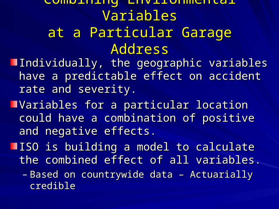
Combining Environmental VariablesCombining Environmental Variablesat a Particular Garage Addressat a Particular Garage Address

Individually, the geographic variables have a Individually, the geographic variables have a predictable effect on accident rate and predictable effect on accident rate and severity.severity.

Variables for a particular location could have Variables for a particular location could have a combination of positive and negative a combination of positive and negative effects.effects.

ISO is building a model to calculate the ISO is building a model to calculate the combined effect of all variables.combined effect of all variables.– Based on countrywide data – Actuarially credibleBased on countrywide data – Actuarially credible

Environmental ModelEnvironmental Model

Loss Cost = Pure Premium

= Frequency x Severity

Frequency = 1

e

e

= Intercept

+ Weather

+ Traffic Density

+ Traffic Generators

+ Traffic Composition

+ Experience and Trend

Environmental ModelEnvironmental Model

Loss Cost = Pure Premium

= Frequency x Severity

Severity = e

= Intercept

+ Weather

+ Traffic Density

+ Traffic Generators

+ Traffic Composition

+ Experience and Trend

Environmental ModelEnvironmental Model

Score = Pure Premium

= Frequency x Severity

Separate Models by CoverageSeparate Models by Coverage– Bodily Injury LiabilityBodily Injury Liability– No-Fault No-Fault – Property Damage LiabilityProperty Damage Liability– CollisionCollision– ComprehensiveComprehensive

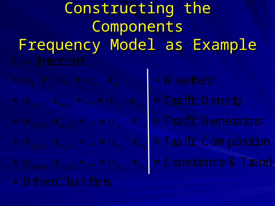
Constructing the ComponentsConstructing the ComponentsFrequency Model as ExampleFrequency Model as Example

1 1

1 1 2 2

2 2 3 3

3 3 4 4

4 4 5 5

1 1

1 1

1 1

1 1

1 1

Intercept

Other Classifiers

n n

n n n n

n n n n

n n n n

n n n n

x ... x

x ... x

x ... x

x ... x

x ... x

= Weather

= Traffic Density

= Traffic Generators

= Traffic Composition

= Experience & Trend

Constructing the ComponentsConstructing the ComponentsFrequency Model as ExampleFrequency Model as Example

““Other Classifiers” reflect driver, vehicle, Other Classifiers” reflect driver, vehicle, limits and deductibles.limits and deductibles.

Model output is deployed to a base class, Model output is deployed to a base class, standard limits and deductibles.standard limits and deductibles.

Data Used in Building ModelData Used in Building Model

Additional Insurer Data – Development PartnersAdditional Insurer Data – Development Partners– From leading insurersFrom leading insurers

Third-Party DataThird-Party Data– TrafficTraffic– Business LocationBusiness Location– DemographicDemographic– WeatherWeather– etcetc

Approximately 1,000 indicatorsApproximately 1,000 indicators

Environmental Module Environmental Module ExamplesExamples

Weather:Weather:– Measures of snowfall, rainfall, Measures of snowfall, rainfall,

temperature, wind and elevationtemperature, wind and elevation

Traffic Density and Driving Traffic Density and Driving PatternsPatterns::– Commute patternsCommute patterns– Public transportation usagePublic transportation usage– Population densityPopulation density– Types of housingTypes of housing

Traffic CompositionTraffic Composition– Demographic groupsDemographic groups– Household sizeHousehold size– HomeownershipHomeownership

Traffic GeneratorsTraffic Generators– Transportation hubsTransportation hubs– Shopping centersShopping centers– Hospitals/medical centersHospitals/medical centers– Entertainment districtsEntertainment districts

Experience and trend:Experience and trend:– ISO loss costISO loss cost– State frequency and severity State frequency and severity

trends from ISO lost cost analysistrends from ISO lost cost analysis

Comprised of over 1000 indicators

Modeling Techniques Modeling Techniques EmployedEmployed

Variable Selection – univariate analysis, Variable Selection – univariate analysis, transformations, known relationship to transformations, known relationship to lossloss

SamplingSampling

Sub models/data reduction – neural nets, Sub models/data reduction – neural nets, splines, principal component analysis, splines, principal component analysis, variable clusteringvariable clustering

Spatial Smoothing – with parameters Spatial Smoothing – with parameters related to auto insurance loss patternsrelated to auto insurance loss patterns

In Depth for Weather In Depth for Weather ComponentComponent

Coverage

Frequency Severity

Traffic Generators

Experience and Trend

Traffic Density

WeatherTraffic

Composition

Neural NetWeather Model 1

Neural Net Weather Model 2

Weather Severity Scale 2

Temperature Model

Weather Severity Scale 1

Weather SummaryVariables

35 Years ofWeather Data

Environmental Model Loss Cost

by Coverage

Frequency×

Severity

Causes of Loss Frequency

Sub Model

Data Summary Variable

Raw Data

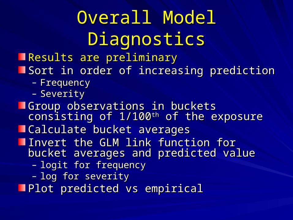
Overall Model DiagnosticsOverall Model Diagnostics

Results are preliminaryResults are preliminarySort in order of increasing predictionSort in order of increasing prediction– FrequencyFrequency– SeveritySeverity

Group observations in buckets consisting of Group observations in buckets consisting of 1/1001/100thth of the exposure of the exposureCalculate bucket averagesCalculate bucket averagesInvert the GLM link function for bucket averages Invert the GLM link function for bucket averages and predicted valueand predicted value– logit for frequencylogit for frequency– log for severitylog for severity

Plot predicted vs empiricalPlot predicted vs empirical

-8 -7 -6 -5 -4 -3

predicted.logit

-8

-7

-6

-5

-4

-3

em

pir

ical.l

ogit

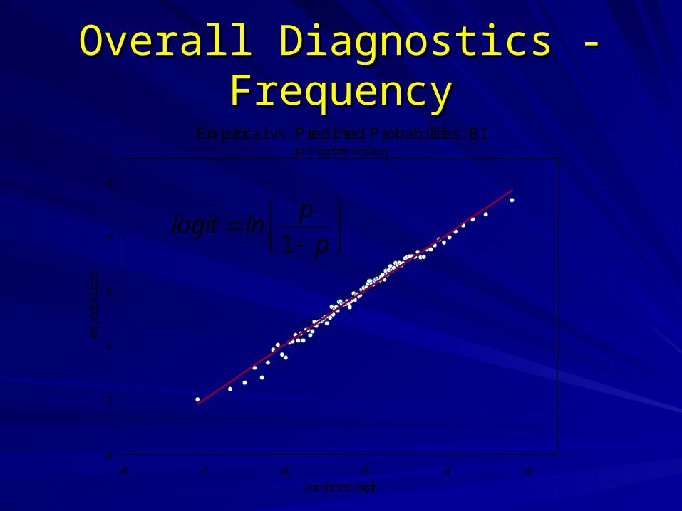
Empirical vs. Predicted Probabilities: BI(On logistic scales)

Overall Diagnostics - FrequencyOverall Diagnostics - Frequency

1

plogit ln

p

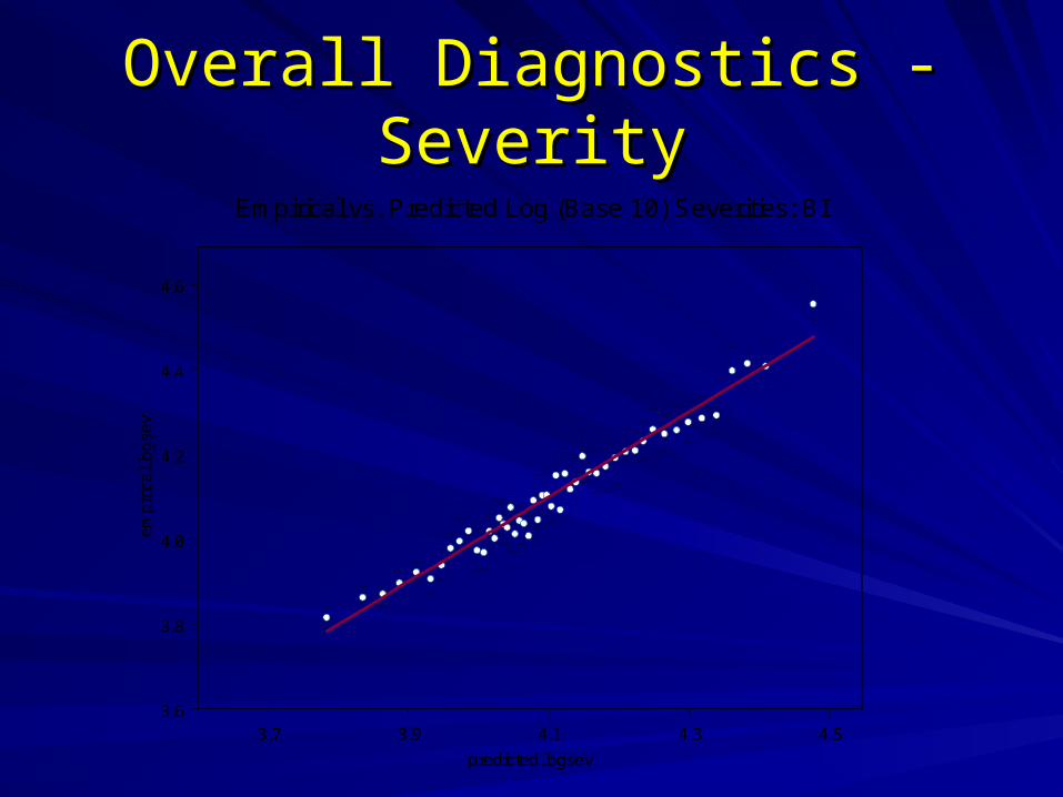
Overall Diagnostics - SeverityOverall Diagnostics - Severity

3.7 3.9 4.1 4.3 4.5

predicted.logsev

3.6

3.8

4.0

4.2

4.4

4.6

em

pir

ical.l

ogse

v

Empirical vs. Predicted Log (Base 10) Severities: BI

Component DiagnosticsComponent DiagnosticsFrequency ExampleFrequency Example

Sort observations in order of Sort observations in order of CCii

Bucket as above and calculate Bucket as above and calculate – CCibib = Average = Average CCii in bucket in bucket bb– ppibib = Average = Average ppii in bucket in bucket bb– Partial Residuals Partial Residuals

Plot Plot CCibib vs vs RRibib – Expect linear relationship – Expect linear relationship

1ib

ib kk iib

pR ln C

p

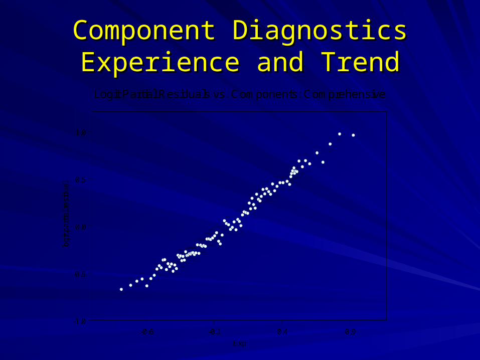
Component DiagnosticsComponent DiagnosticsExperience and TrendExperience and Trend

-0.6 -0.1 0.4 0.9

Exp

-1.0

-0.5

0.0

0.5

1.0

log

it.pa

rtia

l.resi

dual

Logit Partial Residuals vs. Components: Comprehensive

Component DiagnosticsComponent DiagnosticsTraffic CompositionTraffic Composition

-0.16 -0.11 -0.06 -0.01 0.04 0.09 0.14 0.19

TrafComp

-0.4

-0.2

0.0

0.2

0.4

log

it.pa

rtia

l.resi

dual

Logit Partial Residuals vs. Components: Comprehensive

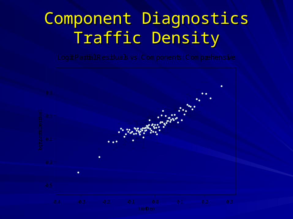
Component DiagnosticsComponent DiagnosticsTraffic DensityTraffic Density

-0.4 -0.3 -0.2 -0.1 0.0 0.1 0.2 0.3

TrafDen

-0.5

-0.3

-0.1

0.1

0.3

log

it.pa

rtia

l.resi

dual

Logit Partial Residuals vs. Components: Comprehensive

Component DiagnosticsComponent DiagnosticsTraffic GeneratorsTraffic Generators

-0.26 -0.21 -0.16 -0.11 -0.06 -0.01 0.04 0.09

TrafGen

-0.5

-0.3

-0.1

0.1

0.3

log

it.part

ial.r

esi

dual

Logit Partial Residuals vs. Components: Comprehensive

Component DiagnosticsComponent DiagnosticsWeatherWeather

-0.4 -0.2 0.0 0.2

Weather

-0.5

-0.3

-0.1

0.1

0.3

0.5

log

it.pa

rtia

l.resi

dual

Logit Partial Residuals vs. Components: Comprehensive

Relativities to Current Loss CostsRelativities to Current Loss Costs

0.7 0.8 0.9 1 1.1 1.2 1.3

BI Relativity

Relativity

% P

rem

ium

020

40

0.7 0.8 0.9 1 1.1 1.2 1.3

PD Relativity

Relativity

% P

rem

ium

020

50

0.7 0.8 0.9 1 1.1 1.2 1.3

Comp Relativity

Relativity

% P

rem

ium

010

25

0.7 0.8 0.9 1 1.1 1.2 1.3

Collision Relativity

Relativity

% P

rem

ium

020

40

Newark NJ AreaNewark NJ AreaCombined RelativityCombined Relativity

"8

"8

"8

"8

"8

"8

"8

"8

"8

"8

"8

"8"8

"8

"8

"8

"8

"8

"8"8

"8

"8

"8

"8

"8

"8 "8

"8

"8

"8

"8

"8

"8

"8

"8

"8

"8

"8"8

"8

"8"8

Clark

Union

Kearny

Linden

Newark

Nutley

Orange

Summit

Verona

Bayonne

Hoboken

Passaic

RoselleCranford

Fairview

Harrison

Hillside

Millburn

Secaucus

Elizabeth

Irvington

Lyndhurst

Maplewood

Montclair

Westfield

Belleville

Bloomfield

GuttenbergLivingston

RidgefieldRutherford

Union City

WallingtonCedar Grove

East Orange

Jersey City

Springfield

West Orange

Little Ferry

Roselle Park

South Orange

Scotch Plains

West Caldwell

West New York

Palisades Park

North Arlington

Ridgefield Park

Evaluating the Lift of Evaluating the Lift of the Environmental Modelthe Environmental Model

Demonstrate the ability to select the more Demonstrate the ability to select the more profitable risksprofitable risksDemonstrate the adverse effect of Demonstrate the adverse effect of competitors “skimming the cream”competitors “skimming the cream”Calculate the “Value of Lift” statisticCalculate the “Value of Lift” statistic

Once insurers see the value of lift other Once insurers see the value of lift other actions are possibleactions are possible– Change prices (etc)Change prices (etc)

Effect of Selecting Effect of Selecting Lower RelativitiesLower Relativities

75 80 85 90 95

Selective Underwriting for BI

% Premium Selected

% D

ecre

ase

in L

oss

Rat

io

01

23

45

6

75 80 85 90 95

Selective Underwriting for PD

% Premium Selected

% D

ecre

ase

in L

oss

Rat

io

01

23

45

6

75 80 85 90 95

Selective Underwriting for Comp

% Premium Selected

% D

ecre

ase

in L

oss

Rat

io

01

23

45

6

75 80 85 90 95

Selective Underwriting for Coll

% Premium Selected

% D

ecre

ase

in L

oss

Rat

io

01

23

45

6

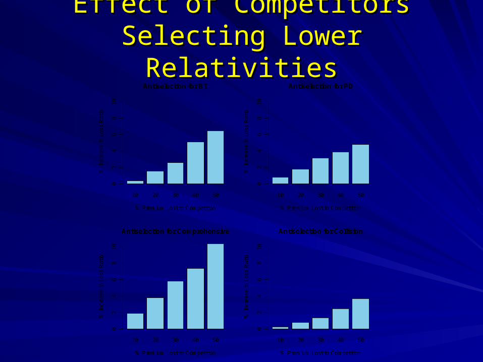
Effect of CompetitorsEffect of CompetitorsSelecting Lower RelativitiesSelecting Lower Relativities

10 20 30 40 50

Antiselection for BI

% Premium Lost to Competition

% I

ncre

ase

in L

oss

Rat

io

02

46

810

10 20 30 40 50

Antiselection for PD

% Premium Lost to Competition

% I

ncre

ase

in L

oss

Rat

io

02

46

810

10 20 30 40 50

Antiselection for Comprehensive

% Premium Lost to Competition

% I

ncre

ase

in L

oss

Rat

io

02

46

810

10 20 30 40 50

Antiselection for Collision

% Premium Lost to Competition

% I

ncre

ase

in L

oss

Rat

io

02

46

810

Assumptions of The FormulaAssumptions of The FormulaValue of Lift (VoL)Value of Lift (VoL)

Assume a competitor comes in and takes away Assume a competitor comes in and takes away the business that is less than your class the business that is less than your class average.average.

Because of adverse selection, the new loss ratio Because of adverse selection, the new loss ratio will be higher than the current loss ratio.will be higher than the current loss ratio.

What is the value of avoiding this fate?What is the value of avoiding this fate?

VoL is proportional to the difference between the VoL is proportional to the difference between the new and the current loss ratio.new and the current loss ratio.

Express the VoL as a $ per car year. Express the VoL as a $ per car year.

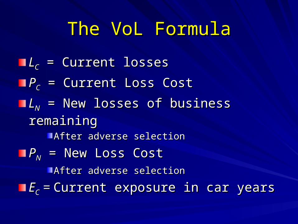
The VoL FormulaThe VoL Formula

LLCC = Current losses = Current losses

PPCC = Current Loss Cost = Current Loss Cost

LLNN = New losses of business remaining = New losses of business remainingAfter adverse selectionAfter adverse selection

PPNN = New Loss Cost = New Loss CostAfter adverse selectionAfter adverse selection

EECC = = Current exposure in car yearsCurrent exposure in car years

The VoL FormulaThe VoL Formula

The numerator represents $ value of the The numerator represents $ value of the potential cost of competitors skimming the potential cost of competitors skimming the cream.cream.

Dividing by Dividing by EECC expresses this value as a $ expresses this value as a $

value per car year.value per car year.

CNN

N C

C

LLP

P PVoL

E

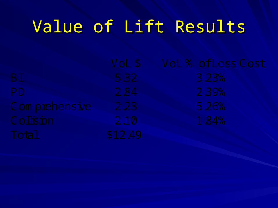
Value of Lift ResultsValue of Lift Results

VoL $ VoL % of Loss CostBI 5.32 3.23%PD 2.84 2.39%Comprehensive 2.23 5.26%Collision 2.10 1.84%Total $12.49

Customized ModelCustomized Model

Loss Cost = Pure Premium

= Frequency x Severity

Frequency = 1

e

e

0

1

2

3

4

5

=

+ Weather

+ Traffic Density

+ Traffic Generators

+ Traffic Composition

+ Experience and Trend

+ Other Classifiers

1 … 5 ≡ 1 in industry model

Severity model customized similarly

Helpful Hints in CustomizationHelpful Hints in Customization

Sample records with no lossesSample records with no losses– Most records have no lossesMost records have no losses

– Attach sample rate, Attach sample rate, ssii, to retained records, to retained records

– Lore is to have equal number of loss records Lore is to have equal number of loss records and no loss records in the sample.and no loss records in the sample.

Policy exposure, Policy exposure, ttii, varies, varies

– Most are 6 month or 12 month policiesMost are 6 month or 12 month policies

Need to account for sampling and exposure in Need to account for sampling and exposure in building modelbuilding model

Sampling and ExposureSampling and Exposurein Logistic Regressionin Logistic Regression

11 1 1i i i i i it s n t s ( n )i i

i

Likelihood ( ( p ) ) ( p )

1 1

i i ii

i i i i i i ii

Loglikelihood s n ln( t )

s n ln( p ) t s ( n )ln( p )

pi = annual probability ni = 1 if claim, 0 if not

ti = policy term si = sample rate

For pi <<1

iiiiit

i ptpoptp i1

2111 ))(1(1)1(1

21 1 1 1iti i i i i i( p ) ( t p o( p )) t p

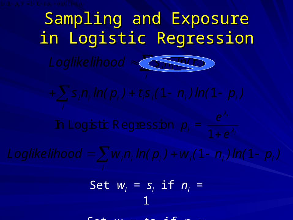
Sampling and ExposureSampling and Exposurein Logistic Regressionin Logistic Regression

1 1

i i ii

i i i i i i ii

Loglikelihood s n ln( t )

s n ln( p ) t s ( n )ln( p )

iiiiit

i ptpoptp i1

2111 ))(1(1)1(1

1 1i i i i i ii

Loglikelihood w n ln( p ) w ( n )ln( p )

In Logistic Regression = 1

i

ii

ep

e

Set wi = si if ni = 1

Set wi = tisi if ni = 0

SummarySummary

Model estimates loss cost as a function of Model estimates loss cost as a function of business, demographic and weather business, demographic and weather conditions.conditions.

Demonstrated model diagnosticsDemonstrated model diagnostics

Demonstrated liftDemonstrated lift

Indicated how to customize the modelIndicated how to customize the model