©2010 Elsevier, Inc. 1 Chapter 7 Cuffey & Paterson

©2010 Elsevier, Inc. 1

Chapter 7Chapter 7

Cuffey & Paterson


FIGURE 7.1

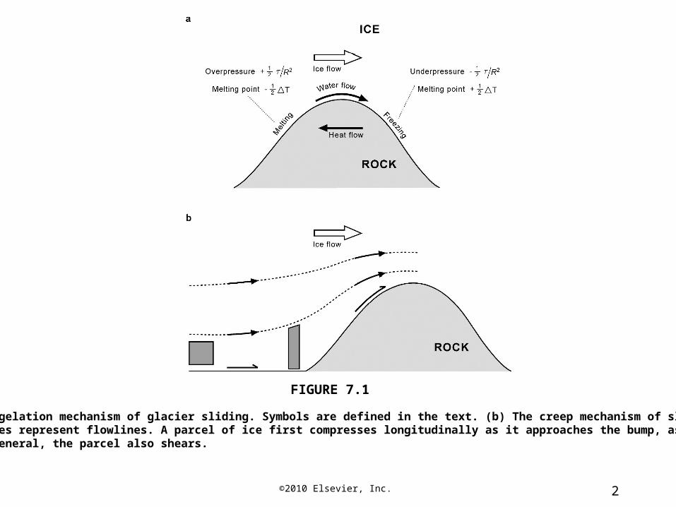
(a) The regelation mechanism of glacier sliding. Symbols are defined in the text. (b) The creep mechanism of sliding. Dashed curves represent flowlines. A parcel of ice first compresses longitudinally as it approaches the bump, as shown. In general, the parcel also shears.


FIGURE 7.2

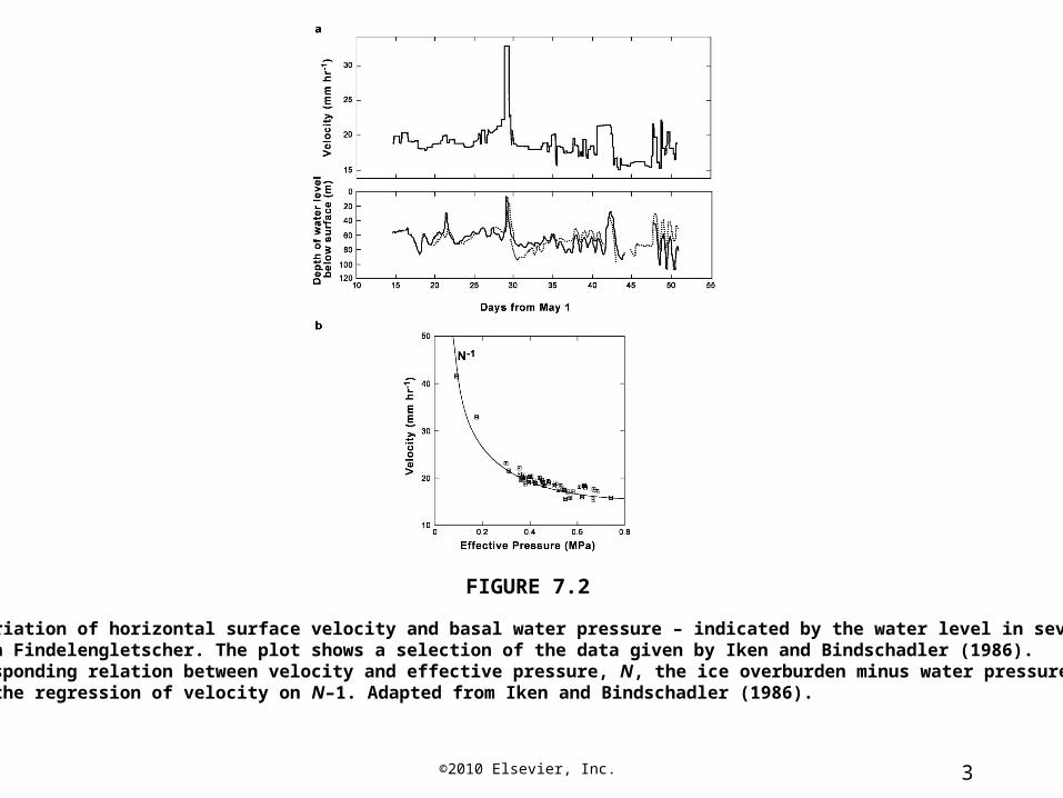
(a) The covariation of horizontal surface velocity and basal water pressure – indicated by the water level in several boreholes – on Findelengletscher. The plot shows a selection of the data given by Iken and Bindschadler (1986). (b) The corresponding relation between velocity and effective pressure, N, the ice overburden minus water pressure. The curve is the regression of velocity on N–1. Adapted from Iken and Bindschadler (1986).


FIGURE 7.3

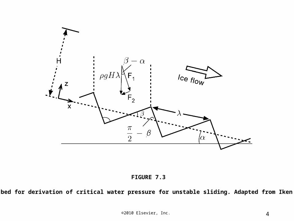
Model of bed for derivation of critical water pressure for unstable sliding. Adapted from Iken (1981).


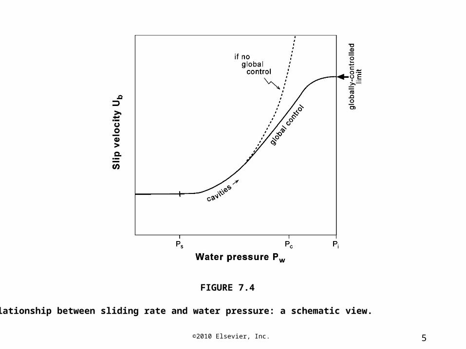
FIGURE 7.4

Relationship between sliding rate and water pressure: a schematic view.


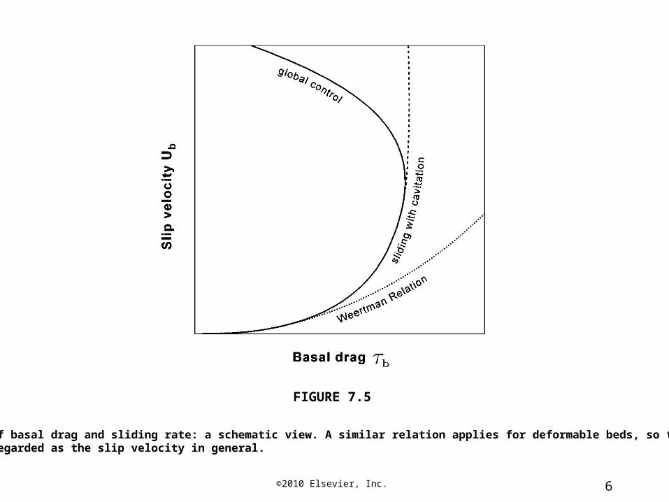
FIGURE 7.5

Covariation of basal drag and sliding rate: a schematic view. A similar relation applies for deformable beds, so the vertical axis can be regarded as the slip velocity in general.


FIGURE 7.6

Measured covariation of sliding velocity and basal water pressure at one site on Lauteraargletscher. Adapted from Sugiyama and Gudmundsson (2004). (a) The day-to-day variations in two periods. Dashed line indicates the overburden pressure. (b) The corresponding relationship of sliding velocity with effective pressure, N, showing faster sliding at times of rising water pressure (N decreasing) compared to times of falling water pressure (N increasing).


FIGURE 7.7

Variables defining the size of a cavity formed on a “tilted staircase” bed. Pi and Pw are ice-overburden and water pressures, Pb the compressive normal stress where ice rests on rock, and τb the overall basal drag. Adapted from Humphrey (1987).


FIGURE 7.8

Covariation of measured basal effective pressure, surface velocity, and bed separation in a 60m × 100m region of Bench Glacier, Alaska. Velocity increased in two phases. The first occurred despite no reduction in effective pressure. The second occurred despite no reduction in effective pressure and no increase in the average separation of ice and bed. The band of velocity values shows the range of measurements at the borehole sites. The other curves are averages for the 17 sites. Adapted from Harper et al. (2007) and used with permission from the American Geophysical Union, Geophysical Research Letters.


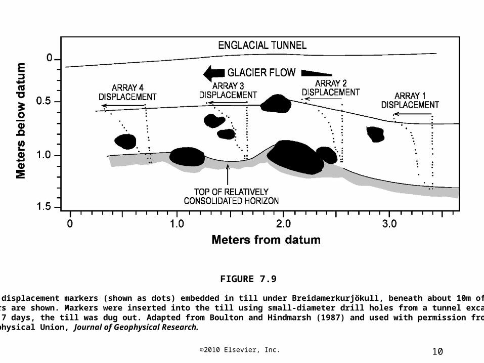
FIGURE 7.9

Positions of displacement markers (shown as dots) embedded in till under Breidamerkurjökull, beneath about 10m of ice. Large boulders are shown. Markers were inserted into the till using small-diameter drill holes from a tunnel excavated in the ice. After 5.7 days, the till was dug out. Adapted from Boulton and Hindmarsh (1987) and used with permission from the American Geophysical Union, Journal of Geophysical Research.


FIGURE 7.10

Horizontal displacements, at six-hour intervals, of strain markers embedded in till under Breidamerkurjökull, beneath about 100m of ice. The spacing between each pattern in the figure is arbitrary, chosen for clarity. Deformation occurs episodically, concentrates near the surface, and tends to propagate downward. Markers were inserted at the bottom of a borehole, using a specialized drill head that emplaced a till core containing the markers, which were attached to drag spools. Adapted from Boulton et al. (2001).


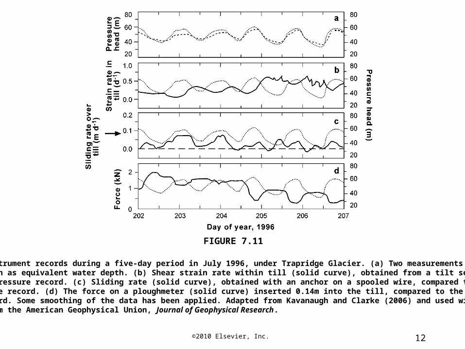
FIGURE 7.11

Subglacial instrument records during a five-day period in July 1996, under Trapridge Glacier. (a) Two measurements of pressure, given as equivalent water depth. (b) Shear strain rate within till (solid curve), obtained from a tilt sensor, compared to one water pressure record. (c) Sliding rate (solid curve), obtained with an anchor on a spooled wire, compared to the same water pressure record. (d) The force on a ploughmeter (solid curve) inserted 0.14m into the till, compared to the same water pressure record. Some smoothing of the data has been applied. Adapted from Kavanaugh and Clarke (2006) and used with permission from the American Geophysical Union, Journal of Geophysical Research.


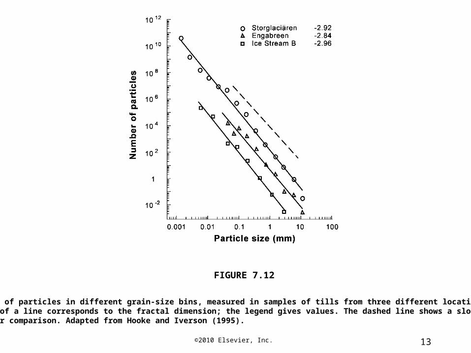
FIGURE 7.12

The number of particles in different grain-size bins, measured in samples of tills from three different locations. The slope of a line corresponds to the fractal dimension; the legend gives values. The dashed line shows a slope of 2.6 for comparison. Adapted from Hooke and Iverson (1995).


FIGURE 7.13

Laboratory measurements of till shear strength, τ*, as a fraction of normal stress. Two different tills were deformed to large strains. The strength does not depend on the rate of shearing, here measured as the rate of displacement at the top of the sample. From Iverson et al. (1998).


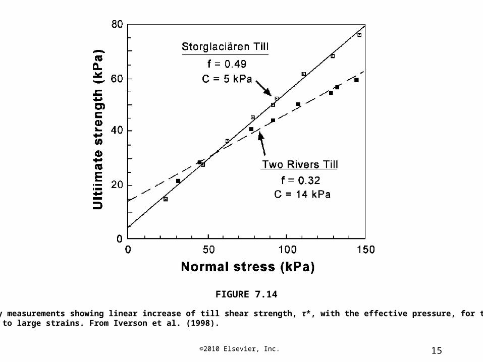
FIGURE 7.14

Laboratory measurements showing linear increase of till shear strength, τ*, with the effective pressure, for two tills deformed to large strains. From Iverson et al. (1998).


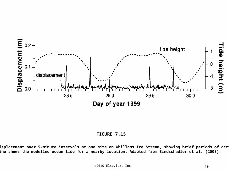
FIGURE 7.15

Horizontal displacement over 5-minute intervals at one site on Whillans Ice Stream, showing brief periods of active slip. The dashed line shows the modelled ocean tide for a nearby location. Adapted from Bindschadler et al. (2003).

Documents

©2010 Elsevier, Inc. 1 Chapter 7 Cuffey & Paterson