2011 MBSW Presentation Statistical Perspectives Based … · 2011 MBSW Presentation Statistical Perspectives Based on a Decade of Experience from Immunogenicity Cut Point Assessments

05/24/2011 Copyright 2011 Bowsher Brunelle Smith, LLC Slide 1

2011 MBSW Presentation

Statistical Perspectives Based on a Decade of Experience from

Immunogenicity Cut Point Assessments

Wendell C. Smith, PhDB2S Consulting™

[email protected] | www.b2s-stats.com


Acknowledgements

Ron Bowsher, B2S Consulting™

Rocco Brunelle, B2S Consulting™

Viswanath Devanarayan, Abbott Laboratories

AAPS-sponsored white papers– Mire-Sluis et al., 2004, JIM (design elements for ADA immunoassays)– Koren et al., 2007, JIM (immunogenicity testing strategy)– Shankar et al., 2008, JPBA (validation of ADA immunoassays)– Gupta et al., 2011, JPBA (NAb assay validation)

Regulatory Guidelines– EMEA guideline on immunogenicity assessment of biotechnology-

derived therapeutics, 2007– FDA draft guidance, 2009


Presentation Outline

Immunogenicity background information– Definition and concerns– Assay methods and test strategy

Cut point study design– Design factors– Sample allocation

Screening cut point data analysis methods– AAPS white paper recommendations – B2S Consulting™ standard approach– Example 1: Direct ELISA– Example 2: Bridging ECL

Cut point application issues


What is immunogenicity?

Ability to provoke an immune response Two (2) types of immunogenicity:

– “Unwanted” (formation of anti-drug antibodies, ADAs)– “Wanted” (formation of antibodies against vaccine antigens)

Unwanted immunogenicity is the major safety concern for biotech drugs

We can not reliably predict ADA incidence or severity of adverse drug reactions (ADR)

Regulatory agencies highly recommend use of a risk-based strategy to evaluate “unwanted” immunogenicity– Risk = Likelihood of developing Abs x Consequence of Ab development– Detection and characterization of ADA is a key component of all strategies


ADA Regulatory Concerns

Concern Clinical Outcome

Safety ADA causes hypersensitivity reactions ADA neutralize activity of an endogenous

equivalent resulting in deficiency syndrome

Efficacy (PD) or in efficacy resulting from a change in biotherapeutic half-life or biodistribution

PK Altered PK caused by ADA results in a

change in dosage level

None Despite ADA generation, there are no

discernable clinical effects /sequelae


Biotech’s Immunogenicity Decade (2000’s)

20052003 2004 20072006 200920082002

AAPS LBABFG Formed (2000)

Crystal City II March 2000

LBABFG IMG Subcommittee

CDER & CBERFDA Re-org

Casadevall et al.NEJM (Feb ‘02)

Mire-Sluis et al.JIM (2004)

FDA DraftGuidance

EMEAGuideline

Shankar et al.JPBA (2008)

Gupta et al.JIM (2007)

Shankar et al.TIBs (2006)

Koren et al.JIM (2008)

AAPS National Biotech Conferences (NBC)

AAPS LBABFG 1st

ImmunogenicityTraining Course

AAPS

Regulatory

Publication

* *


Immunogenicity Testing – 1st White Paper

Numerous statistical design/method recommendations


Immunogenicity Testing – 2nd White Paper


FDA Immunogenicity Draft Guidance

Scope – ADA to Therapeutic Proteins Focus – Clinical investigation Guidance for assays:

ADA detection ADA confirmation Neutralizing Abs

Also relevant for the evaluation of immune data from preclinical studies Not predictive of man Interpretation of Tox / pharm data May reveal potential Ab related tox

FDA supports evolving assay approach


Biotechnology Protein Drugs / Assay Designs

Drug Type Example Assay DesignMonoclonal

AntibodyInfliximab (Remicade), Avastin (Bevacizumab)

Bridging ELISA / ECL

Therapeuticprotein

Erythropoetin (Epogen) hGH (Humatrope)

RIA, ELISA, ECL

Peptide Insulin (Humulin), PTH1-34 (Forteo’)

RIA, ELISA

Fusion Protein Etanercept (Enbrel) ELISA, ECL

Assay Designs AnalyticalResponse

ELISA: Enzyme linked immunosorbant assay Absorbance (OD)ECL: Electrochemiluminescence RLU / ECLRIA / RIPA: Radioimmunoassay %B/T


Assay Design Formats (Monoclonal Ab)

Bridging ELISA Bridging ECL Direct ELISA

Drug

ADA

Biotin-labeled drug

SA-HRP

ADA

HRP-labeledDetection Ab

Drug Fab

ADA

Biotin-labeled drug

Ruthenium-Labeleddrug

SA


‘Uncertainty Principle’ of Anti-Drug Antibody Validations1

Every sample has distinct mixture of isotypes, affinities, avidities (valency), epitope specificities, antibodies conc.

Every sample is likely to differ in these characteristics from every other sample, including the positive control

In normal bioanalysis practice, it is unknown how the characteristics differ from sample-to-sample

Positive Control Sample 1 Sample 21 Courtesy of Bonita Rup, Pfizer


For Immunogenicity applications…

Immunogenicity assays are considered to be Quasi-Quantitative sample result is reported in continuous units of a sample property (i.e., assay signal)

Why?

Reference standards do not exist to reflect the Abaffinities and proportions in patient samples.

Due to the lack of similarity between standard and test samples, use of a calibration curve to report assay results will likely introduce additional error in the identification and quantification of Ab+ samples.


ADA Four-tiered Test Strategy

Tier 1: Identify “reactive” samples– Samples with signal greater than screening cut point

Tier 2: Identify “Ab+” samples by testing reactive samples in the absence and presence of drug– Samples with percent inhibition greater than confirmatory cut point

Tier 3: Determine a sample titer value by serial dilution of Ab+ samples in Tier 2– Titer is based on the screening cut point, and the value can be

either continuous (requires interpolation) or discrete

Tier 4: Evaluate neutralizing effects of antibodies– Based on cell-based bioassay using Ab+ samples


Cut Point Definitions

Screening cut point: Level of assay signal at or above which a sample is defined to be putative positive (‘reactive’) and below which it is defined to be negative.– Determined statistically from the level of binding in drug-naïve

samples– Binding may be nonspecific (due to assay background and sample

matrix components) or specific (due to pre-existing endogenous or anti-drug antibody)

Confirmatory cut point: Level of signal inhibition at or above which a (reactive) sample is judged to have specific anti-drug antibody– Determined by testing (reactive) drug-naïve samples in the absence

and presence of drug


Cut Point Study Design


Cut Point Study Sample Lots ≥ 50 individual drug-naïve normal human serum (NHS)

sample lots – Usually purchased commercially – Usually but not always derived from a single individual– Individuals are assumed to be normal healthy adults and/or having a

specific disease state (i.e. - diabetic)…. no clinical history– Assumed to be drug-naive and antibody negative

Negative base pool (NBP) sample lot– Created by pooling individual lots (after screening)– NBP usually becomes the assay negative control (NC)– Need sufficient volume of NBP to support in-study sample analyses

Low, mid and high positive control lots (LPC, MPC, HPC)– Prepared by spiking the NBP lot with surrogate Ab


Cut Point Study Design Example

Group Lot NumberAnalyst 1 Analyst 2

Run 107-Oct-10

Run 208-Oct-10

Run 311-Oct-10

Run 407-Oct-10

Run 508-Oct-10

Run 611-Oct-10

A (N=17) Plate 1 Plate 3 Plate 2 Plate 1 Plate 3 Plate 2

B (N=17) Plate 2 Plate 1 Plate 3 Plate 2 Plate 1 Plate 3

C (N=17) Plate 3 Plate 2 Plate 1 Plate 3 Plate 2 Plate 1


Study Design Features

Each NHS lot is tested once in each of ≥ 6 assay runs (3 per analyst).

For testing across assay runs, lots are grouped into ‘k’ equal-size subgroups where k is the number of plates in a run.

Lots in a subgroup are tested together on a single plate of each run.

Across runs, each subgroup is tested an equal number of times on the k ordered assay plates.– Latin Square Design


ELISA Cut Point Study: Design Factors

Systematic (Fixed) Effects Subject disease state: NHA, T2D, RA, … Sample lot (assay) group: A, B, C Assay analyst: AAA, BBB Assay plate order: P1, P2, P3

Random Effects Subject sample lot: L1, … , L51

Assay run: R1, R2, R3, …, R6 (3 per analyst) Assay plate: N=18 (3 per run) Residual

Biologicalfactors

Presenter

Presentation Notes

QUESTION: What topics will be covered? Presentation is organized into 4 parts (listed on slide). Give partitioning of slide numbers (4-12, 13-27, 28-36, 37-45) ELISA is used for illustration purposes in order to demonstrate the applicability of principles to assays with a nonlinear calibration curve. Basic issues are similar for all assays.


ELISA Plate Design

Sample assay result– Mean optical density (OD) from 2

wells (adjacent columns)– Result is accepted if CV ≤ 25% for OD

values from 2 wells ?? Number of test samples (drug absent)

– NHS: N = 1 per lot in subgroup– NBP: N ≥ 2 (i.e., 1 each at front,

middle and back of plate)– LPC: N = 2 (i.e., 1 each at two split

plate locations) Maximum number of NHS lots per plate is

less when lots are also tested with drug

96-well ELISAmicrotiter plate8 rows, 12 cols)


Screening Cut Point Data Analysis


Mire-Sluis Illustration (1 run)

Need to log-transform OD values???


Data Analysis Topics (White papers) Target false positive error rate of 5% for screening CP

[versus 0.1% (or 1%) for confirmatory CP] Determine appropriate data transformation Remove samples (lots) with preexisting specific anti-

drug antibodies. Remove statistical “outliers” resulting from non-specific

matrix factors [How about analytical factors?] Confirm distributional assumptions

– Normality– Variance homogeneity

Cut point determinations– Fixed versus floating– Parametric versus nonparametric


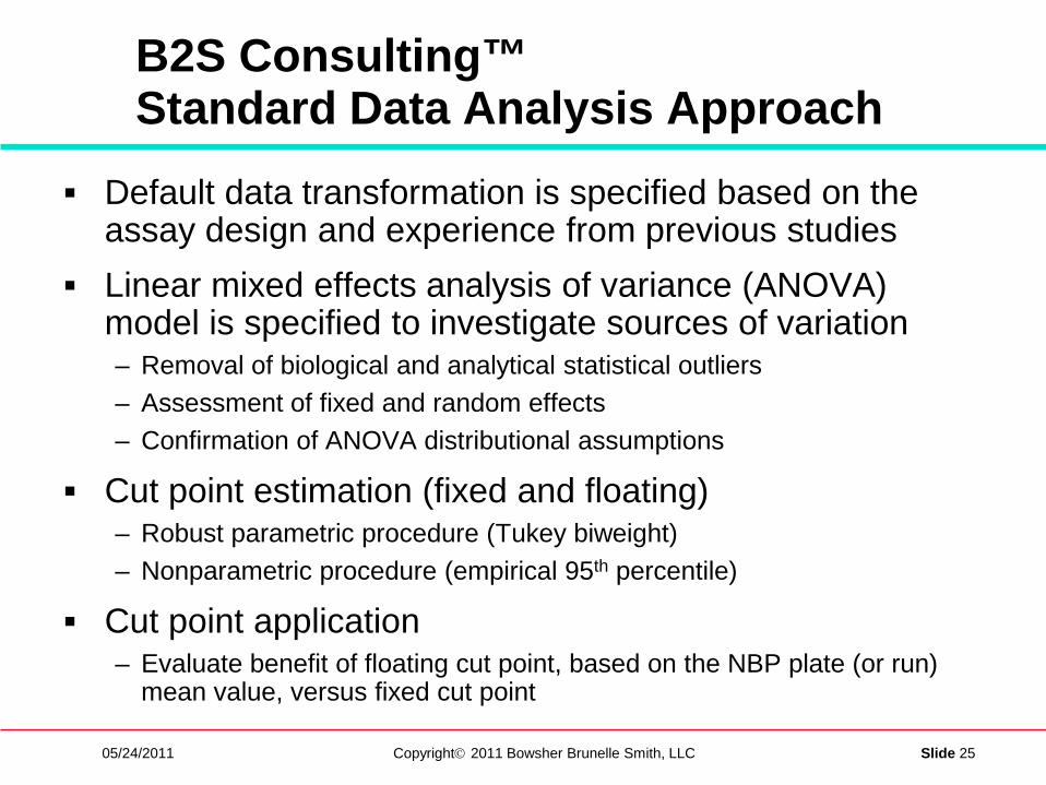
B2S Consulting™ Standard Data Analysis Approach

Default data transformation is specified based on the assay design and experience from previous studies

Linear mixed effects analysis of variance (ANOVA) model is specified to investigate sources of variation– Removal of biological and analytical statistical outliers– Assessment of fixed and random effects– Confirmation of ANOVA distributional assumptions

Cut point estimation (fixed and floating)– Robust parametric procedure (Tukey biweight)– Nonparametric procedure (empirical 95th percentile)

Cut point application– Evaluate benefit of floating cut point, based on the NBP plate (or run)

mean value, versus fixed cut point


Statistical Outliers

Outliers are identified by the “outlier box-plot” criteria– Value > Q3 + 1.5*(Q3-Q1) or < Q1 - 1.5*(Q3-Q1)

» Q3 = 75th percentile, Q1 = 25th percentile (Q2 = median)

Analytical outlier is identified by applying criteria to ANOVA conditional residual values

Biological outlier is identified by applying criteria to sample lot ANOVA best linear unbiased predictor (BLUP) values

Note: Outliers are excluded sequentially (1 at a time?) due to masking and/or lack of independence.


Outlier Illustration (2006 ELISA)

0.10.07

10.7

0.50.4

0.3

0.2

2

Run

#4

.1 .08 .06 1 .8 .6 .5 .4 .3 .2 2

Run #1

Analytical “outlier”

Biological “outlier”

Note: Biological outlier signals are not inhibited by drug. Mean OD for LPC is ~ 0.316.


Screening Cut Point Data AnalysisExample 1: Direct ELISA


Example 1: Study Design


Run 107-Oct-10

Run 208-Oct-10

Run 311-Oct-10

Run 407-Oct-10

Run 508-Oct-10

Run 611-Oct-10





Example 1: Data-related Comments

Total of 306 optical density (OD) values– 51 NHS sample lots (from drug-naïve NHA)– 6 assay runs

Fourteen (14) values were excluded because CV>25% for OD from duplicate wells

Twelve (12) values were excluded as statistical outliers based on the linear mixed effects ANOVA of log (base 10) transformed OD values– 6 individual values identified as analytical outliers– 6 values from one lot identified as a biological outlier


Example 1: Data Scatterplot

-1.1

-1

-0.9

-0.8

-0.7

-0.6

-0.5

-0.4

-0.3

logO

D

1_1

1_2

1_3

2_1

2_2

2_3

3_1

3_2

3_3

4_1

4_2

4_3

5_1

5_2

5_3

6_1

6_2

6_3

Run_Plate

Biologicaloutlier

Analyticaloutlier

CV > 25%


Example 1: Run 4 versus Run 1

0.100.08

0.06

0.20

0.30

0.40

0.50

0.60

Run

4

.10 .08 .06 .20 .30 .40 .50 .60

Run 1

Biologicaloutliers

Analyticaloutlier

CV > 25%

Note: LPC mean OD is ~0.440.


Example 1: ANOVA Random Effects

Random EffectVarianceEstimate

VarianceRatio

PercentOf Total

Lot(Group) 0.020226 10.31 88.87

Run(Analyst) 0.000000 0.00 0.00

Assay Plate 0.000573 0.29 2.51

Residual 0.001961 1.00 8.62

Total 0.022760 - 100.0


Example 1: ANOVA Fixed Effects

Fixed Effect Num DF Den DF P-value

Group 2 52.2 0.541

Analyst 1 10.0 0.236

Plate Order 2 10.0 0.562

Analyst*Plate Order 2 10.0 0.816

Diagnostic tests:> Normality of BLUPs (Shapiro-Wilk p-value = 0.093)> Normality of conditional residuals (S-W p-value = 0.137)> Intra-plate variance homogeneity (Levene p-value = 0.830)


Example 1: Cut Point Estimates

Statistical Method Data Level Fixed (OD)

Floating (Ratio1 )

ParametricClassical All plates 0.261 2.21

Biweight All plates 0.250 2.10Run level 2 0.251 2.13

Nonparametric Biweight All plates 0.299 2.54Run level 2 0.311 2.61

1 Ratio is calculated by dividing each NHS OD value by the NBP geometric mean for the plate (or run for run level estimates)

2 Cut point is determined for each run and then pooled to obtain overall value (Shankar white paper)


Example 1: Fixed Cut Point

-1.1

-1.0

-0.9

-0.8

-0.7

-0.6

-0.5

-0.4

-0.3

logO

D

1_1

1_2

1_3

2_1

2_2

2_3

3_1

3_2

3_3

4_1

4_2

4_3

5_1

5_2

5_3

6_1

6_2

6_3

Run_Plate

BIWT (0.250)

NONP (0.299)


Example 1: Floating Cut Point Factor

-0.2

-0.1

0.0

0.1

0.2

0.3

0.4

0.5

0.6

logR

atio

1_1

1_2

1_3

2_1

2_2

2_3

3_1

3_2

3_3

4_1

4_2

4_3

5_1

5_2

5_3

6_1

6_2

6_3

Run_Plate

NONP (2.54)

BIWT (2.10)


Example 1: Plate mean values

-1.00

-0.96

-0.92

-0.88

-0.84

-0.80

-0.76N

HS

Mea

n (lo

gOD

)

-1.02 -0.98 -0.94 -0.90 -0.86NBP Mean (logOD)

Linear FitLinear Fit

UnconstrainedConstrained (slope=1.0)

Line of equality


Example 1: Histogram of log OD Values

Fitted Normal

Goodness-of-Fit Test

0.968963W

<.0001 *Prob<W

Shapiro-Wilk W Test

-1.1 -1 -0.9 -0.8 -0.7 -0.6 -0.5 -0.4 -0.3

Note: Normality p-value is 0.087 if values from 3 higher lots are excluded (lots are biological outliers in 2-factor random effects model).


Sources of Non- normality

Inappropriate data transformation– log-transformation generally works well

Presence of a few samples with relatively high signals that are not excluded as outliers (previous slide)

Significant difference between mean signal values among levels of an analytical fixed effect factor (i.e., analyst, plate order, …)– Mean difference is often explained by NBP floating cut point

Significant difference between mean signal values among levels of a biological fixed effect factor (i.e., disease state, gender,…)– Mean difference is not explained by NBP consider separate cut

points


Screening Cut Point Data AnalysisExample 2: Bridging ECL


Example 2: Study Design


Run 129-Jun-10

Run 230-Jun-10

Run 301-Jul-10

Run 429-Jun-10

Run 502-Jul-10

Run 601-Jul-10





Example 2: Data-related Comments

Total of 306 optical density (OD) values– 51 NHS sample lots (from drug-naïve NHA)– 6 assay runs

Zero (0) values excluded because of high CV

Thirty-eight (38) values excluded as statistical outliers based on linear mixed effects ANOVA of log (base 10) transformed OD values– 8 individual values identified as analytical outliers– 30 values from five (5) lots identified as biological outliers


Example 2: Data Scatterplot

Biologicaloutlier

Analyticaloutlier

CV > 25%

1.65

1.70

1.75

1.80

1.85

1.90

1.95

2.00

logE

CL

1_1

1_2

1_3

2_1

2_2

2_3

3_1

3_2

3_3

4_1

4_2

4_3

5_1

5_2

5_3

6_1

6_2

6_3

Run_Plate


Example 2: Run 6 versus Run 1

100

90

80

70

60

50

Run

6

100 80 70 60 50 40

Run 1

Biologicaloutlier

Analyticaloutlier

CV > 25%Run 1,Plate 1


Example 2: ANOVA Random Effects

Random EffectVarianceEstimate

VarianceRatio

PercentOf Total

Lot(Group) 0.000030 0.07 1.00

Run(Analyst) 0.001040 2.42 34.64

Assay Plate 0.001501 3.49 50.02

Residual 0.000430 1.00 14.34

Total 0.003001 - 100.0


Example 2: ANOVA Fixed Effects

Fixed Effect Num DF Den DF P-value

Group 2 6.1 0.641

Analyst 1 4.1 0.112

Plate Order 2 6.0 0.653

Analyst*Plate Order 2 6.0 0.689

Diagnostic tests:> Normality of BLUPs (Shapiro-Wilk p-value = 0.842)> Normality of conditional residuals (S-W p-value = 0.608)> Intra-plate variance homogeneity (Levene p-value = 0.033) p < 0.001

at run level


Example 2: Cut Point Estimates

Statistical Method Data Level Fixed (ECL)

Floating (Ratio1 )

ParametricClassical All plates 91.7 1.15

Biweight All plates 92.3 1.14Run level 2 85.2 1.17

Nonparametric Biweight All plates 91.0 1.17Run level 2 84.1 1.17

1 Ratio is calculated by dividing each NHS ECL value by the NBP geometric mean for the plate (or run for run level estimates)

2 Cut point is determined for each run and then pooled to obtain overall value (Shankar white paper)


Example 2: Fixed Cut Point

BIWT (92.3)

NONP (91.0)

1.601.65

1.70

1.75

1.801.85

1.90

1.95

2.002.05

logE

CL

1_1

1_2

1_3

2_1

2_2

2_3

3_1

3_2

3_3

4_1

4_2

4_3

5_1

5_2

5_3

6_1

6_2

6_3

Run_Plate


Example 2: Floating Cut Point Factor

NONP (1.17)

BIWT (1.14)

-0.06

-0.04

-0.02

0.00

0.02

0.04

0.06

0.08

0.10

logR

atio

1_1

1_2

1_3

2_1

2_2

2_3

3_1

3_2

3_3

4_1

4_2

4_3

5_1

5_2

5_3

6_1

6_2

6_3

Run_Plate


Example 2: Plate mean values

1.70

1.75

1.80

1.85

1.90

1.95

2.00N

HS

Mea

n lo

gEC

L

1.70 1.75 1.80 1.85 1.90 1.95 2.00NBP Mean logECL

Linear FitLinear Fit

UnconstrainedConstrained (slope=1.0

NBP low (N=1)


Cut Point Application


Application Issues

Tier 1 screen (ADA Detection)– Is a cut point based on drug-naïve samples useful when the lot variance

component is near 0? Should cut point be based on LPC?– Is a fixed cut point needed when laboratory scientists almost always prefer

a (multiplicative) floating cut point?– How useful is a multiplicative floating cut point factor ≤ 1.0 negative

control will be positive if equivalent to NBP– How should a cut point be determined and applied when the signal

distribution for sample lots is bimodal (i.e., due to high percentage of samples with endogenous antibody present)?

– Should the cut point be adjusted as a result of reagent changes (i.e., new conjugation lot)? If so, how?

• Tier 2 inhibition (ADA Confirmation)– Does it make sense to calculate a confirmatory cut point based on a 0.1%

target false positive error rate when only 50 lots are tested?


Summary / Conclusion

BiotherapeuticAttributes

AssayDesign

Assay Characteristics

StatisticalAnalysis

2000 2011

Assay Design ELISA ECL

Assay Background High Low

Variance High Low

Sources of Variation Biologic > Analytic Analytic > Biologic

Advancement in biotherapeutics will lead to assay evolution which will drive progress indata-driven assignment of immunogenicity CPs

Documents

2011 MBSW Presentation Statistical Perspectives Based … · 2011 MBSW Presentation Statistical Perspectives Based on a Decade of Experience from Immunogenicity Cut Point Assessments