2012 Sales Conference Theme and Team Building - Cerfacs

© 2011 ANSYS, Inc. September 18, 2013

1

Heat transfer Predictions using Scale Resolving Simulation Turbulence Models

F.R. Menter ANSYS Germany GmbH


2

Motivation for Scale-Resolving Simulations (SRS)

• Accuracy Improvements over

RANS Reduce uncertainty in CFD simulations relative

to RANS

Flows with large separation zones (stalled

airfoils/wings, flow past buildings, flows with

swirl instabilities, etc.)

• Additional information required Acoustics - Information on acoustic spectrum not

reliable from RANS

Vortex cavitation – low pressure inside vortex

causes cavitation – resolution of vortex required

Fluid-Structure Interaction (FSI) – unsteady

forces determine frequency response of solid.


3

• RANS Models 1-eq.,

2-eq,

RSM,

EARSM

Transition

…

Turbulence Models

• LES Models Smagorinsky (reg.,

dyn)

WALE

k-equation (dyn.)

WMLES

• Hybrid Models SAS

• All w-equation based models

DES/DDES/IDDES

• SA-based

• SST-based

• k-e based

Zonal/Embedded Models


4

Scale-Adaptive Simulation (SAS) 2-Equation Model

• With: Lk

22

1 2 32

1''

j tk t

j

UP L U k

t x k y y

2 2'

' ; '' ;''

i i i ivK

j j j j k k

U U U U UU U L

x x x x x x U

vKLyU

yUL

22 /

/~

v. Karman length-scale as natural length-scale:

3/ 23/ 4j t

k

j j k j

U kk k kP c

t x L x x

1/ 4

t c

Also transformed to SST

URANS

SAS


5

Detached Eddy Simulation (DES) for SST – Strelets (2000)

3/2( )( )( )

j tk

j t j j

U kk k kP

t x L x x

k-equation RANS

k-equation LES 3/2( )( )

( )j t

k

j DES j j

U kk k kP

t x C x x

k-equation DES

3/2( )( )( )

min ;

j tk

j t DES j j

U kk k kP

t x L C x x

RANS

LES ? cLt

cLt


6

• Smagorinsky model (Smagorinsky, 1963) Need ad-hoc near wall damping

• WALE model (Nicoud & Ducros 1999) Correct asymptotic near wall behaviour

• Dynamic model (Germano et al., 1991) Local adaptation of the Smagorinsky constant

• Dynamic sub-grid kinetic energy transport model (Kim & Menon 2001) (Fluent only) Robust constant calculation procedure Physical limitation of backscatter

2

t sv C S

3/ 2

2

5/ 45/ 2

d d

ij ij

t sd d

ij ij ij ij

S SC

S S S S

2/1

sgskt kCv

j

sgs

k

sgs

j

sgs

j

iij

j

sgsjsgs

x

k

x

kC

x

u

x

ku

t

k

e

2/3

12

3ij kk ij t ijv S

2

t Dv C S

LES Models: Summary

Sub-grid stress : turbulent viscosity


7

Unstructured Hex Mesh NACA 0012

Leading edge Trailing edge

• Re=106

• Span: 0.05 chord; 80 nodes

• In total ~ 11.4 Mio nodes • WALE LES model • Periodicity in spanwise

direction


8

Q-criterion (W2-S2): Q=109 , colored by z-velocity:

WALE Model LES

Leading edge Trailing edge

• Due to high Re number and moderate a, it looks still ok near trailing edge even though span=0.05c


9

5%chord, 11M cells, t=1.5 s

Pressure and skin friction coefficients

Even on this grid cf is too low -> WMLES (see later)

0.000

0.005

0.010

0.015

0.020

0.0 0.2 0.4 0.6 0.8 1.0

Cf

x/chord

Cf comparison: 2-D SST transition vs. 3-D ELES

2-D RANS

3-D ELES pressureside


10

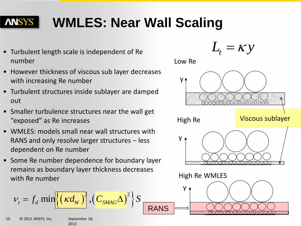
WMLES: Near Wall Scaling

• Turbulent length scale is independent of Re number

• However thickness of viscous sub layer decreases with increasing Re number

• Turbulent structures inside sublayer are damped out

• Smaller turbulence structures near the wall get “exposed” as Re increases

• WMLES: models small near wall structures with RANS and only resolve larger structures – less dependent on Re number

• Some Re number dependence for boundary layer remains as boundary layer thickness decreases with Re number

tL y

Viscous sublayer

Low Re

High Re

y

y

y

High Re WMLES

RANS 2 2

min ,t d W SMAGf d C S


11

WMLES – Channel Flow Tests

Reτ Cells

Number

LES Cells

Number

Nodes

Number

ΔX+ ΔZ+

395 384 000 384 000 81×81×61 40.0 20.0

760 480 000 1 500 000 81×101×61 76.9 38.5

1100 480 000 4 000 000 81×101×61 111.4 55.7

2400 528 000 19 000 000 81×111×61 243.0 121.5

18000 624 000 1 294 676 760 81×131×61 1822.7 911.4

• Very large savings between WMLES and wall-resolved LES

• Alternative is LES with wall functions – however x+ and z+ are a function of y+

RANS Eddy Viscosity


12

• Suitable if zone with high accuracy demands is embedded into larger domain which can be covered properly by RANS models

• Limited zone can then be covered by LES or Wall-Modelled WMLES model

• LES zone needs to be coupled to RANS zone through interfaces

• LES zone requires suitable (WM)LES resolution in time and space

Embedded/Zonal Large Eddy Simulation (ELES)

LES zone

RANS zone

Synthetic Turbulence


13

Zonal LES: Test cases

DIT-x: decay rate validation

Modelled and resolved k


14

Vortex Method

• In essence, vorticity-transport is

modeled by distributing and

tracking many point-vortices on a

plane (Sergent, Bertoglio,

Laurence, 2000)

• Velocity field computed using the

Biot-Savart’s law

xxx

exxxxu

dt z

22

1,

w

ttt k

N

k

k ,,

1

xxx

w


15

Harmonic Turbulence Generator (HTG)

• Input from turbulence model in form of Lt and w.

• Produces Karman spectrum

• Co-operation with Profs. Strelets and Shur (St. Petersburg)

, ,1

ˆˆ2 cosN

i jn n j n n in

u u x t w

HTG RANS LESk k k

2

1

ˆ ,N

n RANS LES

n

u k k

slope k 5/3

Log scale

www

c

kL

Lt

t

,~ˆ,1

~


16

WMLES – Boundary Layer

ReΘ=1000

ReΘ=10000

• Boundary layer simulation: WMLES

Inlet: synthetic turbulence

Vortex Method

2 different Reynolds numbers

ReΘ=1000

ReΘ=10000


17

• Types of highly unstable flows: – Flows with strong swirl instabilities

– Bluff body flows, jet in crossflow

– Massively separated flows

• Physics – Resolved turbulence is generated quickly by flow instability

– Resolved turbulence is not dependent on details of turbulence in upstream RANS region (the RANS model can determine the separation point but from there ‘new’ turbulence is generated)

• Models – SAS: Most easy to use as it converts quickly into LES mode, and

automatically covers the boundary layers in RANS. Has RANS fallback solution in regions not resolved by LES standards (t, x)

– DDES: Similar to SAS, but requires LES resolution for all free shear flows (t, x) (jets etc.)

– ELES: Not really required as RANS model can cover boundary layers. Often difficult to place interfaces for synthetic turbulence.

Flow Types: Globally Unstable Flows

Green-recommended, Red=not recommended


18

• Types of moderately unstable flows: – Jet flows, Mixing layers …

• Physics – Flow instability is weak – RANS/SAS models stay steady state.

– Can typically be covered with reasonable accuracy by RANS models.

– DDES and LES models go unsteady due to the low eddy-viscosity provided by the models. Only works on fine LES quality grids and time steps. Otherwise undefined behavior.

• Models – SAS: Stays in RANS mode. Covers upstream boundary layers in

RANS mode. Can be triggered into SRS mode by RANS-LES interface.

– DDES: Can be triggered to go into LES mode by fine grid and small t. Careful grid generation required. Covers upstream boundary layers in RANS mode.

– ELES: LES mode on fine grid and small t. Careful grid generation required. Upstream boundary layer (pipe flow) in expensive LES mode. Alternative – ELES with synthetic turbulence RANS-LES interface.

Flow Types: Locally Unstable Flows


BL Turbulence

ML Turbulence y

x

z


19

• Types of marginally unstable flows: – Pipe flows, channel flows, boundary layers, ..

• Physics – Transition process is slow and takes several boundary layer

thicknesses.

– When switching from upstream RANS to SRS model, RANS-LES interface with synthetic turbulence generation required.

– RANS-LES interface needs to be placed in non-critical (equilibrium) flow portion. Downstream of interface, full LES resolution required.

• Models – SAS: Stays in RANS mode. Typically good solution with RANS. Can

be triggered into SRS mode by RANS-LES interface.

– DDES: Can be triggered to go into LES mode by fine grid and small t. Careful grid generation required. Covers upstream boundary layers in RANS mode.

– ELES: LES mode on fine grid and small t. Careful grid generation required. Upstream boundary layer (pipe flow) in RANS mode. Synthetic turbulence RANS-LES interface.

Flow Types: Stable Flows



20

Validation of RANS Models

•A comparison between the SST solution and the experimental data for different ReX shows that:

• SST model almost perfectly predicts the temperature profiles for Pr=0.7

• The difference between the SST model and the experimental results is less than 10%

•Hence SST model can be used as a reference solution


21

Virtually the same skin friction distributions are obtained downstream of the step on baseline and uniform 20x20 grids

Grid coarsening leads to “improvement” due to error cancellation

WALE and IDDES models are virtually identical within the separation zone

Grid is sufficient for LES calculations

The difference between WALE and IDDES models upstream and downstream of the separation zone is due to insufficient grid resolution in these regions

Validation: Backward Facing Step


22

Validation: Backward Facing Step •Similar to the BL flow

there is a strong

influence of the grid on

the Stanton number

Grid coarsening in

wall normal direction

leads to substantial

deterioration of the

results

•The Stanton number

distribution for the

WALE model is about

10% lower than those of

IDDES for all the

considered grids

This results are

consistent with

previous observation

for the BL flow


23

Globally Unstable Flow – Jets in Crossflow

Courtesy: Benjamin Duda, Airbus Toulouse

PhD project Benjamin Duda 18 month at Airbus Toulouse (Marie-

Josephe Estève)

18 month ANSYS Germany

(Thorsten Hansen, F. Menter)

Scientific supervisors: Herve Bezard,

Sebastien Deck

Problem: Hot air leaves engine nacelle and

heats wall

Heat shielding required

Experiments too expensive

RANS not accurate enough

Simulations ANSYS-Fluent


24

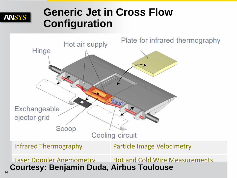
Generic Jet in Cross Flow Configuration

Infrared Thermography Particle Image Velocimetry

Laser Doppler Anemometry Hot and Cold Wire Measurements Courtesy: Benjamin Duda, Airbus Toulouse


25

Hexahedral Mesh

12,900,000 Elements Min angle = 28.1° Max AR = 3,500 Max VC = 10



26

Hybrid Tetrahedral Mesh

21,000,000 Elements Min angle = 20.0° Max AR = 7,600 Max VC = 8

20 inflation layers



27

Hybrid Cartesian Mesh

13,100,000 Elements Min angle = 6.0° 30 Elements < 15° Max AR = 6,000 Max VC = 16

20 inflation layers



28

SAS

Cart

SAS

Tet

Validation Matrix

SAS

Hex

DDES

Hex

ELES

Hex

URANS

Hex

SAS

Hex

SAS

Hex

Time step

Mesh

Turbulence model



29

Scale Resolvability of Turbulence Models

SAS DDES

ELES URANS

Q-criterion:



30

Mean X-Velocity 1 2 3

0

0.2

0.4

0.6

0.8

1

1.2

1.4

1.6

1.8

2

-1 -0.5 0 0.5 1 1.50

0.2

0.4

0.6

0.8

1

1.2

1.4

1.6

1.8

2

0 0.25 0.5 0.75 1 1.25

0

0.2

0.4

0.6

0.8

1

1.2

1.4

1.6

1.8

2

0 0.25 0.5 0.75 1 1.25

URANS SAS M2 SAS M1 EXP

Z w/D

Ej

UU UU UU

X



31

Mean X-Velocity 1 2 3

UU

X

Embedded LES

• Embedded LES (ELES is more consistent at the first station, as expected


32

Time Averaged Temperature Distribution II

Turbulence models (on hex) Lateral spreading of

temperature in good

agreement with all three SRS

Poor URANS prediction due to

unphysical damping of lateral

jet wake movement

Meshing strategies (with

SAS) Generally very good

agreement

Small underestimation for hex

mesh at center

II

TT

TT

j



33

Mean Thermal Efficiency on Wing Surface

EXP

URANS

SAS



34

Heat Conduction in Ejector Grid Solid Domain

Fluid Domain

• Take into account heat

conduction through solid

• Material: stainless steel

• Approach:

Run steady state

computation with heat

transfer

Use surface temperature

distribution as thermal

boundary condition for

transient calculation

• No increase of

computational costs for

transient runs



35

Mean Thermal Efficiency on Wing Surface

SAS, M2

EXP

SAS, M2



36

RMS of X-Velocity on Symmetry Plane

SAS

EXP

U

u 2'

z

x y



37

Hot Jet in Crossflow: Conclusions

• RANS models are not able to reliably predict such flows and are therefore not useful as design tools

• A systematic study was carried out to evaluate SRS models for such applications

• In this study (for several test case configurations) it was found that all SRS methods worked equally well in predicting the main flow characteristics

• On suitable grids (~106 cells) good agreement even in the secondary quantities (stresses) could be achieved

• More complex geometries studied


38

Flow schematic

Branch Pipe: T=36 Q=6 [l/s] =0.1 [m] δBL=0.01 [m]

Main Pipe: T=19 Q=9 [l/s] =0.14 [m] Developed Flow

Water of different temperature is mixing in the T-junction at Re=1.4105 (based on the main pipe bulk velocity and on its diameter)

The target values are mean and RMS wall temperatures in the fatigue zone


39

Isosurfaces of Q-criterion Colored with Temperature for Different SRS Models

• Sensitivity to numerics

depends on the SRS

model

• SAS with BCD is virtually

steady

• The reason is that the flow

is not enough unstable

• Unsteady solution with

resolved turbulent

structures is obtained for

the CD scheme

• For other models the effect

of numerics is not seen

from instantaneous fields


40

Comparison of Different SRS Models

• CD scheme is used for

comparison between

different SRS models

• All models are able to

predict mean and RMS

profiles with sufficient

accuracy


41

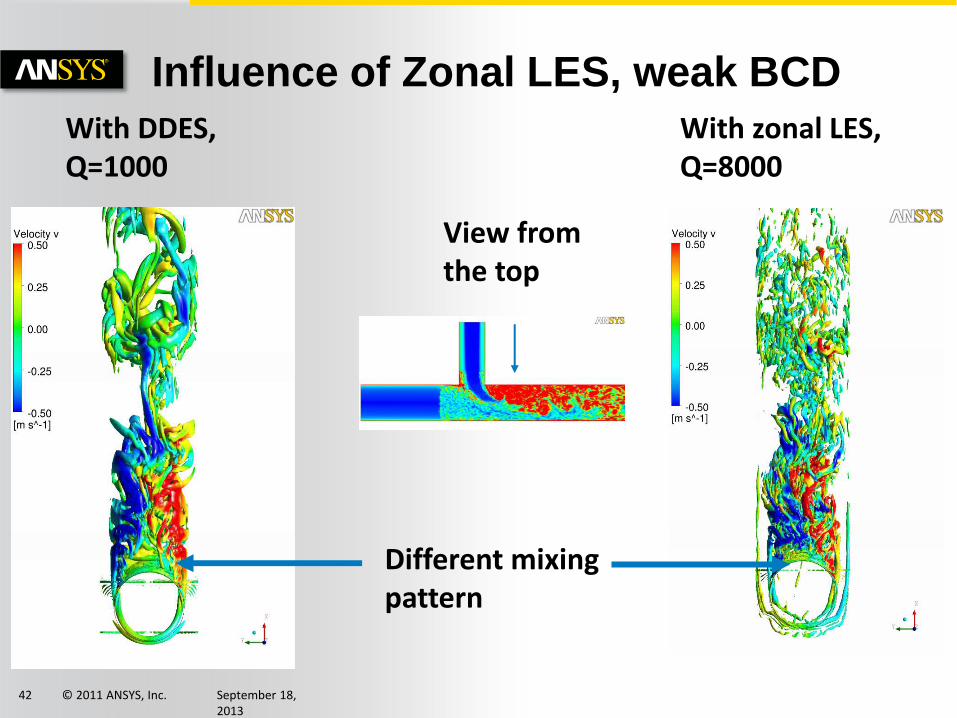
Influence of Zonal LES, weak BCD

Wall temperature in the fatigue zone

Top wall line

• Noticeable differences

appear when looking at

the wall temperature

• All global models failed

to provide the correct

temperature distribution

right past the

intersection

• Only zonal (embedded)

formulation is able to

provide the correct

mixing already from the

start of the mixing zone


42

Influence of Zonal LES, weak BCD

With DDES, Q=1000

With zonal LES, Q=8000

View from the top

Different mixing pattern


43

Overall Summary

• SRS is making its way into industrial CFD

• Heat Transfer Simulations are a key application area for SRS High accuracy requirements

Limited accuracy of RANS models

• Currently favored methods within ANSYS software:

SAS – globally unstable flows

DDES – globally and locally unstable flows

ELES/WMLES stable flows

• Ongoing work: Synthetic turbulence is good – but far from perfect

WMLES requires special grid resolution – not as generic as other

models (inherited from LES)

Improved wall treatment for heat transfer predictions

User guidelines

Documents

2012 Sales Conference Theme and Team Building - Cerfacs