1

2013-2015 National Survey of Family Growth (NSFG): Summary of Design and Data Collection Methods

1. Introduction

2. Background on the National Survey of Family Growth

3. Sample Design3.1 Sample universe

3.2 Sample selection

4. Responsive Design and Management of Fieldwork

5. Data Collection Activities5.1 Interviewer training

5.2 Computer hardware, software, and related supplies

5.3 Fieldwork protocol

5.4 Use of incentives

6. Production Outcomes

7. Data Preparation for Public Use7.1 Imputation of recodes

7.2 Procedures to minimize risk of disclosure for individual-level data

7.3 Weighting and variance estimation

8. Accounting for Complex Sample Design in Analysis

9. References

10. Appendix I: Glossary

2

Introduction

This report provides key methodological information to users and analysts of the 2013-2015 National Survey of Family Growth (NSFG), beyond the information included in the User’s Guide that accompanied the release of these public use files in October 2016. The 2013-2015 NSFG includes two years (eight quarters) of data from the continuous NSFG. This two year period covers the 9th through 16th quarters of an overall 8 year period of planned fieldwork. It follows an initial release of data from the first 8 quarters of interviews that took place between September 2011 and September 2013. See “2011-2013 National Survey of Family Growth (NSFG): Summary of Design and Data Collection Methods” “for an analogous report for that first data release.

This web-based report and related, detailed reports are intended to replace the Series 1 and Series 2 reports formerly published by the National Center for Health Statistics (NCHS), but still permit the timely release of essential information on the sample design and data collection methods for the NSFG. Updated or new reports will be posted periodically on the NSFG webpage as more data are released from the continuously fielded survey.

The NSFG moved from a periodically conducted survey design as conducted by NCHS 6 times from 1973 to 2002, to a continuous survey design in 2006. This transition and new design have been described in prior reports. The following 3 reports document the significant changes made for the 2006-2010 NSFG, as well as providing details on how the survey was planned and designed:

• “Planning and Development of the Continuous National Survey of Family Growth”: describesplanning for and implementation of the transition from a periodic to a continuous survey, priorto the release of the first data from continuous interviewing.

• ”The 2006-2010 National Survey of Family Growth: Sample Design and Analysis of aContinuous Survey”: describes the sample design and weighting and variance estimationprocedures under the continuous design, prior to the release of the first data from continuousinterviewing.

• ”Responsive Design, Weighting, and Variance Estimation in the 2006-2010 National Survey ofFamily Growth”: Presents fieldwork results and weighting, imputation, and variance estimationprocedures corresponding to the first release of data (2006-2010) under the continuous design.

The current report builds upon the information available in these prior reports, notes design differences from the 2006-2010 survey period, summarizes updated production outcomes for 2013-2015, and describes the weighting, variance estimation, imputation, and disclosure risk review and operations that took place to produce the public use datasets for analysis. This report and three detailed reports for 2013-2015 mirror the same set of reports accompanying the 2011-2013 datasets. Thus each of the two sets of reports are intended to be “stand-alone”, containing the same level of comprehensiveness, with this set of reports including information specific to the 2013-2015 dataset. Where relevant, specific outcomes from the 2011-2013 NSFG are provided alongside those for 2013-2015 for comparison purposes.

3

Background on the National Survey of Family Growth

For background information on the purpose, content, and sponsorship of the NSFG, please see the main NSFG webpage, specifically the “About NSFG” section and the User’s Guide for 2013-2015.

As with the 2006-2010 NSFG and 2011-2013 NSFG, the 2013-2015 NSFG was conducted by the University of Michigan’s Institute for Social Research under a contract with NCHS. Interviewing for the 2013-2015 survey began in mid- September 2013 and continued through early September 2015 yielding data files spanning two years (or eight quarters) of interviews. Interviews were conducted with a national probability sample of women and men 15-44 years of age living in households in the United States. The interviews were administered in person by trained female interviewers using laptop computers, a procedure called computer-assisted personal interviewing (CAPI). A subset of the more sensitive questions was administered using audio-computer assisted self-interviewing (Audio-CASI or ACASI). In this procedure, respondents answer the questions on the laptop computer, either by reading them on the screen or listening to the pre-recorded questions read over headphones, and enter their answers directly into the computer. The interviews for women averaged 74.5 minutes, and the interviews for men averaged about 49.5 minutes, remaining within the OMB-approved lengths of 80 minutes for women and 60 minutes for men. About 5% (512 out of 10,210 interviews) were completed in Spanish, which is the only other language accommodated in the NSFG design.

Sample Design

This document provides a brief overview of the NSFG sample design. A more detailed description of the sampling procedures can be found here.

The NSFG sample was designed to meet a number of key objectives including: 1) minimizing the overall design effects for women and men2) controlling the costs of both screening and interviewing3) obtaining overall sample size of at least 5,000 interviews per year4) providing for oversamples of non-Hispanic blacks, Hispanics, and teens aged 15-19

Further, the continuous design was planned to provide annual, nationally representative samples, permitting data to be cumulated over multiple years of continuous interviewing. However, the weights provided are based on a minimum of 2 years’ worth of interviews, due to the limited sample sizes in single years of interviewing. To obtain sample sizes comparable to 2006-2010 and prior NSFG file releases, data from the 2011-2013 NSFG and 2013-2015 NSFG can be combined. Documentation on combining data from the 2011-2013 and 2013-2015 files can be found in the User’s Guide for 2013-2015, Appendix 2, under “Combining Data Across NSFG File Releases”. Within this appendix is a section containing information specific to the 2011-2013 and 2013-2015 files combined, or the “2011-2015” field period.

4

Sample universe

The survey population, or population of inference, for the 2013-2015 NSFG consists of all non-institutionalized women and men ages 15-44 years as of first contact for the survey, and whose usual place of residence is the 50 United States and the District of Columbia. Excluded from the survey population are those in institutions, such as prisons, homes for juvenile delinquents, homes for the intellectually disabled, long-term psychiatric hospitals, and those living on military bases. Included in the sample are age eligible persons living in non-institutional group quarters (e.g., dormitories, fraternities), college students sampled through their parent or guardians’ households, and women and men who are in the military but living off base.

Sample selection

The NSFG is based on a stratified multi-stage area probability sample, using probability proportionate to size (PPS) selection within each of four key domains, as shown below in Table 1. There are five stages of sample selection:

1) selection of primary sampling units (PSUs)2) selection of secondary sampling units (SSUs)3) listing and selection of housing units within SSUs4) selecting one of the eligible persons within each sampled household5) two-phase sampling for nonresponse

These five stages are briefly outlined below. Data from the 2010 decennial census were used as the sampling frame for the first two stages of selection.

1) Selection of Primary Sampling Units

The first stage involved the selection of Primary Sampling Units (PSUs). PSUs are Metropolitan Statistical Areas (MSAs), counties or groups of counties. The United States was divided into 2,149 PSUs on the sampling frame. Of these, 366 are MSAs and 1,783 are non-MSA PSUs that include one or more counties. The PSUs are stratified according to attributes such as Census Division, MSA status, and size. One or two PSUs are selected with probability proportionate to size (PPS) from each stratum. The PPS selection method assigns higher probabilities to PSUs with larger populations. The first stage selection probabilities are inversely related to the probabilities of selection at the second and third stages of selection such that sampling rates are approximately equal for all households within a sampling domain (defined below). Across the 8 years of data collection (2011-2019) there are a total of 21 “self-representing” (SR) PSUs, defined as PSUs that were automatically included in national probability samples due to their large population, and an additional 192 non-self-representing (NSR) PSUs, defined as PSUs selected into the NSFG sample that represents not only themselves but other non-self-representing PSUs, for a total of 213 PSUs, plus 2 for Alaska and Hawaii. A subset of these 215 PSUs is selected for each 2-year sampling period. For 2013-2015, there are 65 PSUs: 17 SR and 48 NSR PSUs.

In order to facilitate the oversample of subgroups defined by race and ethnicity, the measures of size for the PSUs were a weighted combination of household counts. All Census Block groups were classified into four sampling “domains” shown in Table 1. Households in domains 2, 3, and 4 were given a higher probability of selection than those in domain 1. These weighted measures of size are then used in both the first and second stages of selection.

5

Table 1. Domain definitions and characteristics

Domain Definition Total Households Est. Proportion Black

Est. Proportion Hispanic

1 <10% HH Black, <10% HH Hispanic

65,009,685 0.018 0.022

2 >=10% HH Black, <10% HH Hispanic

19,871,976 0.426 0.029

3 <10% HH Black, >=10% HH Hispanic

20,270,438 0.026 0.380

4 >=10% HH Black, >=10% HH Hispanic

11,564,193 0.301 0.299

NOTE: HH stands for “household”.

2) Selection of Secondary Sampling Units

In the second stage of selection, Secondary Sampling Units (SSUs or segments) are selected within PSUs. These are composed of one or more Census blocks with a minimum measure of size equal to 50 housing units (HUs). SSUs in domains 2, 3, and 4 have relatively higher combined PSU, SSU, and HU selection rates. These weighted measures of size and sampling rates are set such that interviews with black and Hispanic respondents each constitute about 20% of all interviews. Each PSU is assigned one or two ISR interviewers based on its relative size. For each interviewer, 12 SSUs are selected each year. These SSUs are then randomly divided into 4 groups, with one group of 3 SSUs assigned to each calendar quarter.

3) Listing and Selection of Housing Units within SSU’s

For the third stage of selection, interviewers updated commercially-available lists (based on the U.S. Postal Service’s Delivery Sequence File (DSF)) of housing units for SSUs where these lists are available or, alternatively, created such a list from scratch where they are not available. Once these lists were updated, a sample of housing units was selected systematically from geographically-sorted lists of housing units, beginning from a random start.

Beginning in Quarter 13 (2013), a sample design change was implemented with the goal of increasing the percentage of screened households that contain an eligible person. This was accomplished by stratifying housing units based on a prediction of whether the unit contained an eligible person. The model was selected and estimated using data from previous quarters where the binary eligibility outcome was measured. Key predictors in this model included commercial data that estimate whether an eligible person is in the household. The predicted probability of there being an eligible person in the household was used to create strata and then oversample the stratum or strata with higher expected eligibility.

The selected units were then contacted by ISR interviewers to determine if any members of the household were eligible (persons age 15-44 at the time of the screening interview). A full household roster was obtained during the screening interview to identify eligible household members.

4) Selection of Eligible Persons

6

In households with eligible persons, a fourth stage of selection involved selecting one of the eligible persons. The within-household selection rates were set so that about 20% of all interviews are with teens aged 15-19 and 55% of all interviews are with females.

5) Two-Phase Sampling for Nonresponse

As was done in the 2006-2010 NSFG and 2011-2013 NSFG, the 2013-2015 NSFG also used a two-phase sampling approach as a fifth stage of selection. Each quarter, during week 10, a subsample of active cases was selected for continued follow-up. In weeks 11 and 12, this subsample received a special mailed incentive and the interviewers focused their effort on the fewer cases left in the subsample. Details of this two-phase design are described in Lepkowski et al. (2013) and further below.

Responsive Design and Management of Fieldwork

The NSFG sample selection and the fieldwork procedures are designed around an interviewer labor model of 38 “workloads” each quarter, with an expectation of each interviewer working at least 30 hours a week for four quarters. A “workload” refers to the average person-time that each interviewer is expected and budgeted to work. It is best accomplished as 38 interviewers each working for 30 hours per week and meeting production goals during the 12 week period. This can also be accomplished with more than 38 interviewers who may work for slightly fewer hours per week, or fewer interviewers working more hours per week. The number of sample lines is adjusted each quarter, based on predicted interviewer-level efficiency, to ensure that each interviewer has sufficient sample to support a workload.

Hiring and training interviewers for at least one year of work (in the NSR PSUs) and guaranteeing them a workload of at least 30 hours a week are intended to minimize attrition and results in a more stable interviewer workforce.

The NSFG utilizes a responsive design each quarter. The overall goals of the responsive design approach are to balance response rates across key subgroups (defined by gender, race/ethnicity and age) and manage the costs of data collection. Details of the responsive design approach are provided elsewhere. Key elements of the responsive design approach include:

• Quarterly data collection with replicates (random subsamples of each annual sample)• Two phases of data collection each quarter• Sample design around interviewer workloads to maximize efficiency• Daily monitoring of key fieldwork indicators• Planned interventions to direct interviewer effort at specific points in space and time

As noted above, Phase 1 data collection comprised the first 10 weeks of data collection in each quarter. In that time, all sample cases are made available to interviewers, who are directed to focus attention on cases not yet screened or cases already screened and ready for the main interview, depending on what the fieldwork indicators show. In week 10 of each quarter a subsample of about 1/3 of cases is selected for continued effort in Phase 2 (weeks 11 and 12). Interviewer assignments are reduced so that interviewers can concentrate effort on a smaller number of housing units and selected persons for the

7

final two weeks of data collection while maintaining their overall number of hours worked. This two-phase subsampling design has been critical for controlling final response rates and costs.

Data Collection Activities

This section describes the fieldwork protocols used for NSFG data collection. Interviewer training is first briefly described, followed by a description of the computer equipment used for NSFG. The respondent recruitment or fieldwork protocol is then described. Many of the details of the process are the same as, or similar to, those used for the 2006-2010 NSFG fieldwork (see Groves et al., 2009) and are the same as those used in the 2011-2013 NSFG.

Interviewer training

Under the current contract for the continuous NSFG 2011-2019, interviewer training has been conducted in September each year, as that is the start of the interviewing period for each year. Interviewers were trained in a centralized location near the contractor’s home office in Ann Arbor, MI, where the full ISR staff of NSFG is available to assist. NCHS NSFG staff also participated in all training sessions. In 2011, the first year of fieldwork under the new contract, all 50 interviewers attended training. In 2013, only those 20 who were new to the project attended interviewer training, and in 2014, 17 interviewers new to NSFG attended training.

Interviewer training consisted of a home study portion completed prior to attending training, a 1.5 day general interviewing techniques (GIT) training for all newly hired interviewers, 5 days of study specific training and a certification interview that all interviewers were required to successfully complete before beginning fieldwork. Bilingual interviewers also completed an additional half-day training session. The home study portion of training included on-line videos and sections of the study manual to review, and an assessment to complete prior to attending in-person training. Study specific training was conducted primarily in smaller groups and focused on the following topics:

• Reviewing and practicing household listing and screening• Administering the male and female questionnaires using carefully planned “mock” interview

scripts and hands-on practice with the interviewer aids such as the show card booklet and lifehistory calendar

• Learning and practicing various study protocols such as addressing common respondentconcerns and “averting refusals”

• Learning other administrative tasks such as entering their time and expense reports.

Computer hardware, software, and related supplies

The computers used in the NSFG in 2013-2015 were Fujitsu Lifebook tablet computers. Computer supplies included an AC adaptor, a car adaptor, an extra laptop battery and headphones for use during the ACASI portion of the interview. Interviewers were also provided with a locking laptop case and shredders for secure disposal of any paper materials bearing confidential information.

As in the 2006-2010 NSFG and 2011-2013 NSFG, both screener and main interviews for 2013-2015 were conducted using computer assisted personal interviewing (CAPI), with audio computer-assisted survey interviewing (ACASI) for the most sensitive questions. The entire interview was programmed in the

8

Blaise software (version 4.8) developed by Statistics Netherlands. A change introduced in 2011 involved the use of text-to-speech (TTS, or computer-generated) voice files for the ACASI instruments, rather than a recorded human voice, as used in prior years of NSFG (Couper et al., 2015).

Fieldwork protocol

The fieldwork protocol utilized in 2013-2015 was essentially the same as the protocol used in 2006-2010 (see Groves et al. 2009) and 2011-2013. These procedures were reviewed and approved by the Ethics Review Board (ERB) at NCHS and also reviewed by the University of Michigan Institutional Review Board. The key steps in the recruitment protocol were:

1. An advance household letter and an NSFG Question-and-Answer Brochure were mailed to allselected housing units prior to initiating in-person contact. The letter was printed in English onone side and Spanish on the other, but for the purpose of this description, the Phase 1 andPhase 2 English letters are shown.

2. If no one was home on the first visit, a “Sorry I Missed You” card was left at the householdindicating that the interviewer had stopped by and would return at another time. Return visitswere made to households during a different time of day or different day of the week than theinitial contact. If a household member was not willing to complete the screening interview atthat time, the interviewer answered any questions regarding the survey and the process andoffered to return at a more convenient time.

3. When contact was made with a sampled household, the field interviewer introduced herself tothe household member by displaying her identification badge and identifying that she was aninterviewer from the University of Michigan contacting the household on behalf of the NationalSurvey of Family Growth. The advance household letter was referenced and the letter ofauthorization was shown if necessary.

4. Once establishing that the household member was an adult 18 or older and willing to participatein the brief (less than 5 minutes) household screener, the interviewer conducted the householdscreener to determine if any household member was age-eligible for the survey. If more thanone age-eligible household member was identified, the pre-programmed survey selectionalgorithm selected one person to be interviewed. If no one in the household was eligible, nofurther contact was made with the household. Age was the primary basis for ineligibility,however in some cases an age-eligible household member may have been ruled out on the basisof language or other factors. Due to resource and sample size constraints, the NSFG interviewcould only be conducted in English or Spanish.

5. Once selected to participate, adult respondents were provided with a respondent letterexplaining that they had been selected for the survey and a copy of the informed consent form,covering all required elements of informed consent. The interviewer asked if they were willingto participate in the survey, and if so, they were asked to provide an electronic signatureacknowledging informed consent, and provided a $40 token of appreciation in advance ofcompleting the interview. Adult respondents were not required to sign the electronic consentform, as the NSFG was granted a waiver of documentation of informed consent by the NCHSERB, and in the event they chose not to sign, the interviewer signed the consent form to

9

acknowledge that informed consent information was provided and the respondent agreed to participate.

6. In the case where the selected respondent was a minor, defined as ages 15-17 in most states,signed informed consent and permission was first requested of a parent of the minorrespondent prior to talking with him or her. Once parental consent and permission wereobtained, the minor was provided with a letter explaining that they had been selected for thesurvey. The minor was provided a copy of the minor assent form, asked to provide an electronicsignature acknowledging their assent, and then provided a $40 token of appreciation in advanceof completing the interview. Unlike the case with adult respondents, a signature from theminor’s parent on the parent permission form and a signature from the minor respondent onthe minor assent form were both required in order to proceed with the minor’s interview.

7. The main interview was conducted in a private setting with the interviewer reading thequestions and entering the responses in the laptop. A private setting was defined as having noone over the age of 4 years within hearing range of the interviewer and respondent. Variousaids were used throughout the interview: show cards that the respondent referred to forresponse categories; question-by-question guidance (“help screens”)for the interviewer to readto the respondent if additional information was needed on a particular question; and the LifeHistory Calendar used only for female respondents as a tool to aid in recalling dates and detailedevents. All respondents were offered headphones to complete the Audio-CASI section of theinterview, but they could choose not to use the headphones and read the questions onscreen ifthey preferred.

8. At the end of the Audio CASI section, the respondent was prompted to lock the interview databefore returning the computer to the interviewer. This locking made it impossible for theinterviewer to back up and view any of the respondents’ answers to ACASI, nor could theinterviewer back up and alter any prior responses to questions she administered before ACASI.Before leaving the household, the interviewer turned off and further locked the computer andthanked the respondent for his/her participation.

Use of incentives

As noted above, respondents in Phase 1 of data collection were offered a $40 token of appreciation, paid in cash. Those screened in Phase 1 and selected into Phase 2 for a main interview were offered an additional $40 (for a total of $80) as a prepaid token of appreciation for completion of the survey. Households selected into Phase 2 that were not yet screened in Phase 1 were also sent a $5 prepaid token of appreciation for completion of the screener. This protocol was based on earlier research on incentives in the NSFG (see Lepkowski et al. 2013, Appendix II).

Production Outcomes

The following series of tables show key production statistics from the 2013-2015 NSFG, with comparable numbers from the 2006-2010 NSFG and 2011-2013 NSFG, where appropriate for comparative purposes.

10

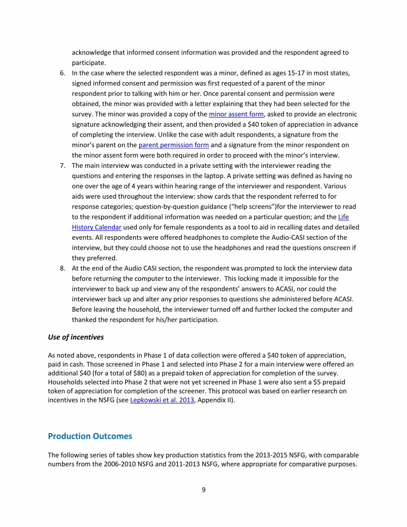
Table 2 provides key summary counts for the overall NSFG sample, as well as averages per quarter of data collection. Table 2. Number of sampled addresses, screened eligible households, and main interviews, and average number of addresses, eligible households, and main interviews per quarter, 2006-2010, 2011-2013, and 2013-2015 NSFG.

2006-2010 2011-2013 2013-2015 Sampled addressesa

Total Average per quarter

78,082 4,880

39,494 4,937

40,598 5,075

Screened eligible householdsb

Total Average per quarter

32,134 2,008

15,287 1,911

15,239 1,905

Main interviewsc Total Average per quarter

22,682 1,418

10,416 1,302

10,178 1,276

aSampled addresses are the number of addresses selected into the screener sample. bScreened eligible households are successfully screened addresses containing one or more age-eligible persons.. cMain interviews are screened eligible households with a completed interview with the selected respondent (including partial interviews which are those where the respondent at least reached the last applicable question before ACASI).

Table 3 presents key indicators of eligibility. The percentages of occupied housing units with eligible persons are lower in 2011-2013 and 2013-2015 than in 2006-2010. The decline in the percent of occupied housing units with eligible persons would have been larger in 2013-2015, but a procedure was implemented starting in 2013 to increase eligibility rates (see Sample Design). Despite this, we still see a modest decline in eligibility rates compared to 2006-2010, reflecting demographic trends in household composition. The lower eligibility rate is also reflected in the lower “yield” of screener and main interview cases in Table 2 above. Also shown in Table 3, the percent of housing units with access impediments increased slightly from 2011-2013 to 2013-2015.

Table 3. Weighted percent of housing units that were occupied, percent of occupied housing units with an age-eligible person, and percent of occupied housing units with access impediments by data collection release, 2006-2010, 2011-2013, and 2013-2015 NSFG.

2006-2010 2011-2013 2013-2015 Percent of all housing units that were occupied

85.6% 84.4% 86.3%

Percent of all occupied households with an age-eligible person 15-44

52.3% 48.8% 47.7%

Percent of occupied housing units with access impediments*

14.1% 13.6% 15.8%

NOTE: Results are based on removal of screener and main lines not selected for the second-phase sample. *Examples of access impediments include locked apartment building doors and gated communities with guards.

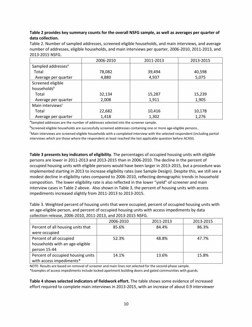
Table 4 shows selected indicators of fieldwork effort. The table shows some evidence of increased effort required to complete main interviews in 2013-2015, with an increase of about 0.9 interviewer

11

hours per completed interview (representing about a 9% increase in effort) relative to 2011-2013. This continues a trend from 2006-2010.

Table 4. Average number of calls (in-person visits) to obtain a screener, a main interview, and the total, and average number of hours of interviewer labor to complete an interview, 2006-2010, 2011-2013, and 2013-15 NSFG.

2006-2010 2011-2013 2013-2015 Number of screener calls to obtain screening interview

3.3 3.3 3.6

Number of main interview calls to obtain main interviewa

4.0 4.3 4.3

Number of total calls to achieve main interviewb

7.2c 7.4c 7.8

Hours of Interviewer labor per completed interview

9.1 9.8 10.7

aMean number of calls per main interview is the average number of main calls on the cases with completed interviews. bMean number of total calls on a case to achieve main interview is the average number of main and screener calls on the cases with completed interviews. cThe average total calls is not equal to the sum of average screener and main calls due to rounding, and the fact that not all completed screener interviews resulted in a main interview.

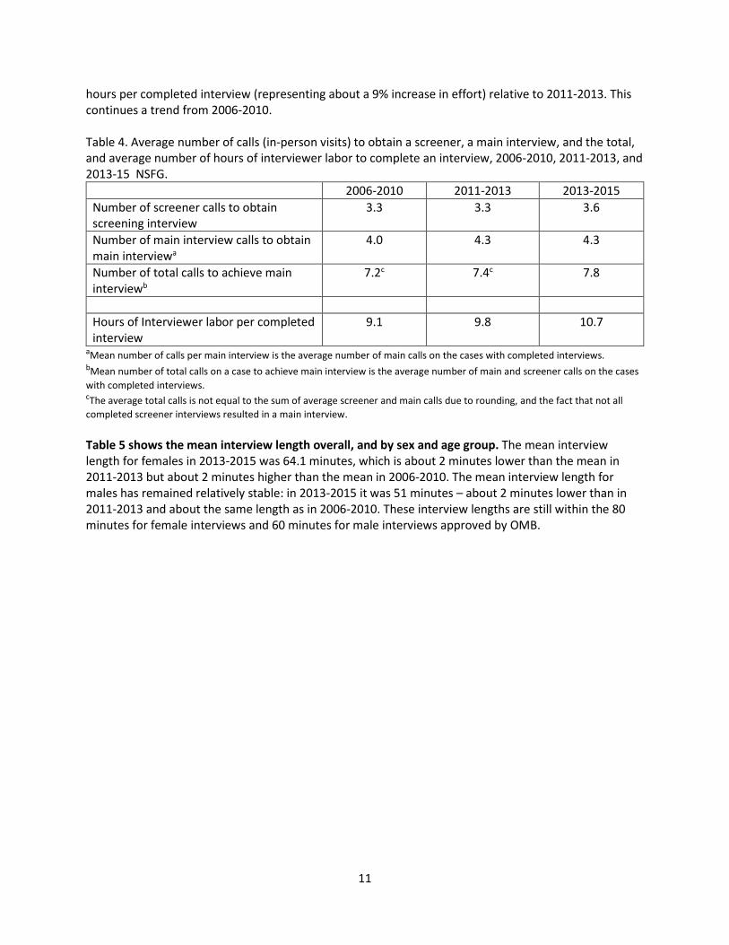
Table 5 shows the mean interview length overall, and by sex and age group. The mean interview length for females in 2013-2015 was 64.1 minutes, which is about 2 minutes lower than the mean in 2011-2013 but about 2 minutes higher than the mean in 2006-2010. The mean interview length for males has remained relatively stable: in 2013-2015 it was 51 minutes – about 2 minutes lower than in 2011-2013 and about the same length as in 2006-2010. These interview lengths are still within the 80 minutes for female interviews and 60 minutes for male interviews approved by OMB.

12

Table 5. Mean and median length of interview in minutes, for completed female and male interviews by age group: 2006-2010, 2011-2013, and 2013-2015 NSFG.

Sex and age Meana and median length of interview in minutes 2006-2010 2011-2013 2013-2015

Total Mean Median

61.6 57.4

66.0 60.9

64.1 59.6

Female Total Mean Median

70.4 67.6

77.5 73.9

74.5 71.8

15-19MeanMedian

52.4 47.8

56.9 51.9

49.5 40.3

20-44MeanMedian

74.6 71.4

82.1 78.3

78.8 75.7

Male Total Mean Median

51.2 48.5

52.8 50.5

51.0 48.4

15-19MeanMedian

41.7 39.3

43.1 40.9

42.4 40.2

20-44MeanMedian

54.0 51.3

55.6 53.4

53.5 50.7

a Means exclude interviews with total lengths greater than 3 standard deviations from the mean.

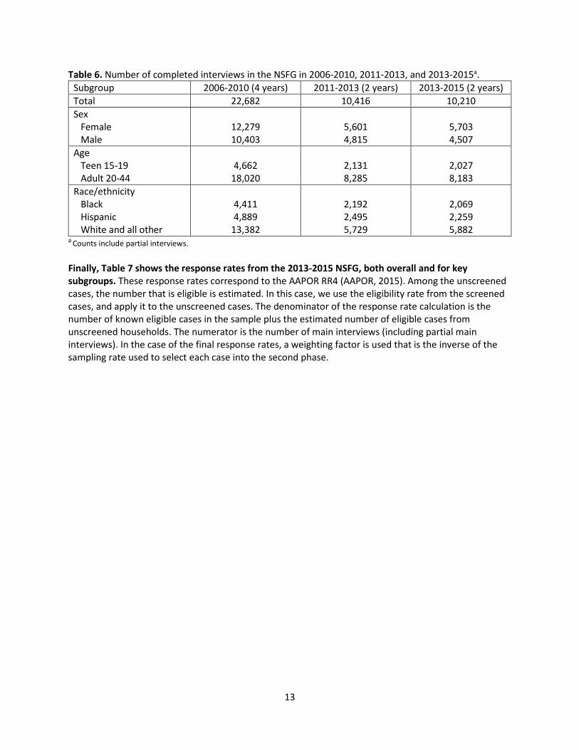
Table 6 contains the final case counts by sex, age and race/ethnicity for the two years (8 quarters) of interview data included in the 2013-2015 NSFG, along with the comparable numbers for 2006-2010 NSFG (4 years or 16 quarters) and 2011-2013 NSFG (2 years or 8 quarters). A total of 10,210 completed interviews or sufficient partial interviews were obtained in 2013-2015. Sufficient partials are cases that are complete at least through the last applicable question before ACASI; some may stop the interview then or stop somewhere during the ACASI component; 32 of the 10,210 interviews were classified as partials.

13

Table 6. Number of completed interviews in the NSFG in 2006-2010, 2011-2013, and 2013-2015a. Subgroup 2006-2010 (4 years) 2011-2013 (2 years) 2013-2015 (2 years) Total 22,682 10,416 10,210 Sex Female Male

12,279 10,403

5,601 4,815

5,703 4,507

Age Teen 15-19 Adult 20-44

4,662 18,020

2,131 8,285

2,027 8,183

Race/ethnicity Black Hispanic White and all other

4,411 4,889

13,382

2,192 2,495 5,729

2,069 2,259 5,882

a Counts include partial interviews.

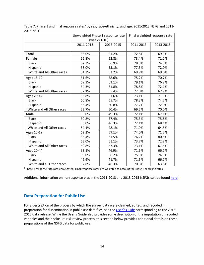
Finally, Table 7 shows the response rates from the 2013-2015 NSFG, both overall and for key subgroups. These response rates correspond to the AAPOR RR4 (AAPOR, 2015). Among the unscreened cases, the number that is eligible is estimated. In this case, we use the eligibility rate from the screened cases, and apply it to the unscreened cases. The denominator of the response rate calculation is the number of known eligible cases in the sample plus the estimated number of eligible cases from unscreened households. The numerator is the number of main interviews (including partial main interviews). In the case of the final response rates, a weighting factor is used that is the inverse of the sampling rate used to select each case into the second phase.

14

Table 7. Phase 1 and final response ratesa by sex, race-ethnicity, and age: 2011-2013 NSFG and 2013-2015 NSFG

Unweighted Phase 1 response rate (weeks 1-10)

Final weighted response rate

2011-2013 2013-2015 2011-2013 2013-2015

Total 56.0% 51.2% 72.8% 69.3% Female 56.8% 52.8% 73.4% 71.2% Black Hispanic White and All Other races

62.3% 58.0% 54.2%

56.9% 53.1% 51.2%

78.5% 77.5% 69.9%

74.5% 72.0% 69.6%

Ages 15-19 Black Hispanic White and All Other races

61.6% 69.3% 64.3% 57.1%

58.6% 63.1% 61.8% 55.4%

75.2% 79.1% 78.8% 72.0%

70.7% 76.2% 72.1% 67.9%

Ages 20-44 Black Hispanic White and All Other races

55.8% 60.8% 56.4% 53.7%

51.6% 55.7% 50.8% 50.4%

73.1% 78.3% 77.2% 69.5%

71.3% 74.2% 72.0% 70.0%

Male 55.0% 49.3% 72.1% 67.1% Black Hispanic White and All Other races

60.8% 53.0% 54.1%

57.4% 46.3% 48.1%

75.5% 72.1% 71.0%

75.8% 68.1% 64.5%

Ages 15-19 Black Hispanic White and All Other races

62.1% 66.4% 63.0% 59.8%

59.1% 61.5% 61.1% 57.3%

74.0% 76.2% 73.7% 73.1%

71.2% 80.5% 72.8% 67.5%

Ages 20-44 Black Hispanic White and all Other races

53.1% 59.0% 49.6% 52.8%

46.9% 56.2% 41.7% 46.3%

71.6% 75.3% 71.6% 70.6%

66.1% 74.5% 66.7% 63.8%

a Phase 1 response rates are unweighted; Final response rates are weighted to account for Phase 2 sampling rates.

Additional information on nonresponse bias in the 2011-2013 and 2013-2015 NSFGs can be found here.

Data Preparation for Public Use

For a description of the process by which the survey data were cleaned, edited, and recoded in preparation for dissemination in public use data files, see the User’s Guide corresponding to the 2013-2015 data release. While the User’s Guide also provides some description of the imputation of recoded variables and the disclosure risk review process, this section below provides additional details on these preparations of the NSFG data for public use.

15

Imputation of recodes

Most missing recode values were assigned using regression imputation software in which multiple regression is used to predict a value for the case using other variables in the data set as predictors. For each variable with missing data, a regression model is estimated to predict the values for the missing data. The predicted values have a stochastic element added to reflect uncertainty in the coefficients of the model and the predictions. Categorical outcomes are stochastically classified into a single category. This process is repeated sequentially several times for all the variables with missing data. For more details on the method used (sequential regression imputation), see Raghunathan et al. (2001). For specific details on how the approach is implemented with the NSFG, see Lepkowski, et al. (2010) and Lepkowski, et al. (2013). Regression imputation follows the same logical constraints that are built into the original recode specifications. To the extent possible, imputed values generated by regression modeling are checked to ensure that the imputed values are within acceptable ranges, and are consistent with other recodes and other data reported by the respondent.

Some cases for some recodes were imputed using logical imputation, which involves having a subject-matter expert at NCHS examine variables related to the variable in question, and assign a value that is consistent with those other variables. Logical imputation is an educated guess of the true value when there is any ambiguity.

The recodes with the highest rate of imputation involved income. Regression imputation was used for about 9.6% of cases for both poverty level (POVERTY) and total household income (TOTINCR). For no other recodes did the percent of values imputed exceed 2% of all cases.

Regardless of whether any values on a recode were imputed, every NSFG recode has a corresponding imputation flag variable indicating whether the value was based on questionnaire data, logical imputation, or regression model-based imputation. These flags, allow users the flexibility to handle imputed cases as they may choose for their own analyses, however it is the recommendation of NCHS that imputed values be retained in analyses to generate consistent point estimates for the population.

Procedures to minimize risk of disclosure for individual-level data

Before any NSFG public use file is released by NCHS, there are a number of steps taken to protect the confidentiality of respondents. First, the NSFG staff modify the data files to prevent disclosure of the identities of the respondents, including the suppression or collapsing of additional variables that could be used to identify very small groups. Next, the proposed NSFG public use files are reviewed by the NCHS Disclosure Review Board (DRB) and the NCHS Confidentiality Officer. Third, in response to the DRB’s review, the NSFG staff and contractor make further changes where necessary to minimize the risk of disclosure. Last, the values of some variables are altered for some respondents in a process called statistical perturbation. Perturbation is a technique that changes the data before dissemination in such a way that the disclosure risk for the data is decreased but the information content is retained as far as possible. Statistical perturbation is done by a separate team of staff at ISR, and details of the perturbation process are kept from other ISR or NCHS staff to preserve the integrity of the process. In general the process involved identifying variables eligible for perturbation, and by determining an appropriate level of perturbation (the proportion of cases whose values may be changed). Once the

16

variables were identified and a perturbation rate determined, a random subset of eligible cases with non-missing values for that variable were deleted. Then the same sequential regression procedure used to impute for missing data (see above description of imputation) was used to impute the values for those cases set to missing. The resulting “perturbed” values were therefore generally based on the same multivariate models used for the imputation process. These perturbed values were then recoded if necessary to be consistent with existing recode specifications. The resulting distributions on each of the perturbed variables were then carefully checked to make sure that the recode specifications were satisfied. The NSFG public use dataset contains the perturbed values for these cases and variables.

Weighting and variance estimation

The development of weights and sample design characteristics for variance estimation are briefly described here. For more detail, see reports on weighting and sampling error estimation codes.

The final analysis weights for the NSFG 2013-2015 include 1) a base weight for the housing unit and person selection probabilities, 2) a nonresponse adjustment, and 3) a post-stratification factor. The weights were also trimmed to control the variance of the weights, since highly variable weights may inflate estimates of standard errors. The base probability of selection is calculated from the five separate stages of sampling described earlier.

In order to adjust for any potential bias, nonresponse adjustment factors were developed. Sample based unit nonresponse adjustments were developed by generating predicted probabilities of response using all available data for respondents and nonrespondents at the screener and main interview levels. Screener and main interview cases will have different response processes. Therefore, we have modeled these separately in the adjustment process. In addition, there is slightly different data available at each level. The information on the unscreened cases is somewhat sparser. It includes data from the Census Block file as well as information from the paradata, in particular, interviewer observations (see documentation on weighting). Once the probabilities of response have been estimated, they were classified into deciles, and the inverse of the response rate within each decile was used as a nonresponse adjustment factor. This was done separately for screener and main probabilities.

The last component of the weight is a post-stratification factor. Post-stratification weights the sample to match population totals known from a source such as the Census. This can reduce sampling error and also may help reduce biases due to nonresponse or noncoverage. The selected factors used for post-stratification were age (in six categories: 15-19, 20-24, 25-29, 30-34, 35-39, and 40-44), sex, and race/ethnicity (in 3 categories: black non-Hispanic, non-black non-Hispanic, and Hispanic). This created 36 (6x2x3) separate cells for which we compared population counts to estimated totals. The post-stratification factor for each cell was the population total divided by the sample estimate of that total.

The base probabilities of selection, nonresponse adjustments, and post-stratification factors were then combined to form a single, final weight: WGT2013_2015. Extreme values of this weight were trimmed in order to reduce the variability of the weights. It is recommended that this weight variable be used for all analyses conducted from the two-year file.

A weight corresponding to the four year period 2011-2015 is also available, named WGT2011_2015. Documentation on combining data from the 2011-2013 and 2013-2015 files to create a file spanning these 4 years can be found in Appendix 2. This appendix also contains guidelines for using weights, explanations of the populations represented by the years of data covered, and example programs for

17

using weights and variables for proper variance estimation. Similarly, variance estimation examples using 4 years of data (2011-2013 and 2013-2015) can be found on the 2013-2015 page, under the title, “2011-2015 Variance Estimation Examples”.

Table 8 shows the mean weights for key subgroups, along with the potential increase in variance due to weighting (as estimated using 1 + L; see Kish, 1992). This measure (1 + L) is a global measure (i.e., not specific to any one variable) that assesses the extent to which the variability of an estimated mean or proportion might be increased because of variability in the weights. A value of 1.0 indicated no contribution to variability due to weighting; a value of 2.0 suggests that there is a potential for the variability of estimate to double due to the weights. After trimming, the minimum weight is 1859.1 and the maximum is 75399.4.

18

Table 8. Mean final weights (after post-stratification to Census data and trimming), and potential increases in variance due to the weights (1 + L), by sex, age group, and race/ethnicity, 2011-2013 and 2013-2015 NSFG.

Sample size Mean weight Increase in variance (1+L) 2011- 2013

2013- 2015

2011- 2013

2013- 2015

2011- 2013

2013- 2015

Total 10416 10205 11655.8 12018.5 2.27 2.03

Male 4815 4506 12569.0 13572.4 2.19 1.93

Female 5601 5699 10870.8 10789.9 2.34 2.10

15 to 19 2131 2027 9272.8 9633.6 2.24 1.89

20 to 44 8285 8178 12268.8 12609.6 2.25 2.03

Hispanic 2495 2258 9370.5 10597.0 2.36 2.10

Black 2192 2068 7803.9 8305.0 2.41 2.07

Other 5729 5879 14125.0 13870.8 2.08 1.92

In addition to differential weighting, the NSFG design is a stratified cluster sample. This stratification and clustering should be accounted for when estimating variance. In order to reflect the sample design as adequately as possible, without risking disclosure of the identity of respondents, we have created pseudo-strata and pseudo-clusters for variance estimation purposes. The clusters are identified by the variable SECU, and are numbered 1, 2, 3, and 4. These SECUs are nested within pseudo-strata, i.e. unique SECUs are identified by the combination of SEST and SECU. The pseudo-strata are contained in the variable SEST. It is recommended that these variables (SEST and SECU) be used for any estimate of variance (see also Guidelines for Analysis below).

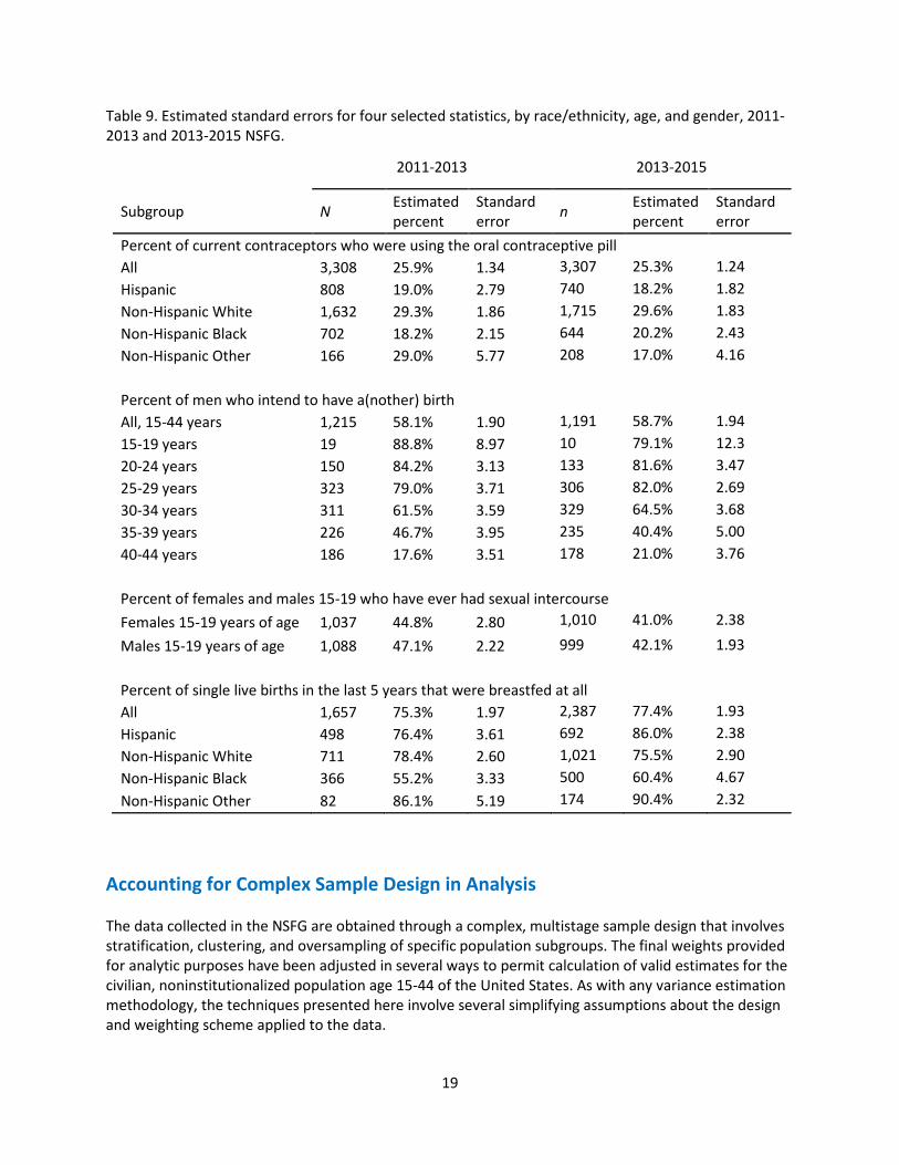
Table 9 shows estimated percentages and standard errors (reflecting the complex design) for four selected statistics, by race/ethnicity, age and gender, for 2011-2013 and 2013-2015 NSFG. These can be compared to estimates from 2002 NSFG and 2006-2010 NSFG Table X in Lepkowski et al. (2013), but remember the latter come from 4 years of data, while the estimates below are from 2 years of data in each data release. The standard errors in the table below are very similar to those from 2 years of data (2008-2010) from the earlier data release.

19

Table 9. Estimated standard errors for four selected statistics, by race/ethnicity, age, and gender, 2011-2013 and 2013-2015 NSFG.

2011-2013 2013-2015

Subgroup N Estimated percent

Standard error n Estimated

percent Standard error

Percent of current contraceptors who were using the oral contraceptive pill All 3,308 25.9% 1.34 3,307 25.3% 1.24 Hispanic 808 19.0% 2.79 740 18.2% 1.82 Non-Hispanic White 1,632 29.3% 1.86 1,715 29.6% 1.83 Non-Hispanic Black 702 18.2% 2.15 644 20.2% 2.43 Non-Hispanic Other 166 29.0% 5.77 208 17.0% 4.16 Percent of men who intend to have a(nother) birth All, 15-44 years 1,215 58.1% 1.90 1,191 58.7% 1.94 15-19 years 19 88.8% 8.97 10 79.1% 12.3 20-24 years 150 84.2% 3.13 133 81.6% 3.47 25-29 years 323 79.0% 3.71 306 82.0% 2.69 30-34 years 311 61.5% 3.59 329 64.5% 3.68 35-39 years 226 46.7% 3.95 235 40.4% 5.00 40-44 years 186 17.6% 3.51 178 21.0% 3.76 Percent of females and males 15-19 who have ever had sexual intercourse Females 15-19 years of age 1,037 44.8% 2.80 1,010 41.0% 2.38

Males 15-19 years of age 1,088 47.1% 2.22 999 42.1% 1.93 Percent of single live births in the last 5 years that were breastfed at all All 1,657 75.3% 1.97 2,387 77.4% 1.93 Hispanic 498 76.4% 3.61 692 86.0% 2.38 Non-Hispanic White 711 78.4% 2.60 1,021 75.5% 2.90 Non-Hispanic Black 366 55.2% 3.33 500 60.4% 4.67 Non-Hispanic Other 82 86.1% 5.19 174 90.4% 2.32

Accounting for Complex Sample Design in Analysis The data collected in the NSFG are obtained through a complex, multistage sample design that involves stratification, clustering, and oversampling of specific population subgroups. The final weights provided for analytic purposes have been adjusted in several ways to permit calculation of valid estimates for the civilian, noninstitutionalized population age 15-44 of the United States. As with any variance estimation methodology, the techniques presented here involve several simplifying assumptions about the design and weighting scheme applied to the data.

20

Data users are reminded that the use of standard statistical procedures that are based on the assumption that data are generated via simple random sampling (SRS) generally will produce incorrect estimates of variances and standard errors when used to analyze data from the NSFG. Analysts who apply SRS techniques to NSFG data generally will produce standard error estimates that are, on average, too small, and are likely to produce results that are subject to excessive Type I error. For further details on analysis of complex sample survey data, see Heeringa, West, and Berglund (2010). Analysts are strongly encouraged to use appropriate software to reflect the complex sample design in their analyses. Several software packages are available for analyzing complex samples. The key design variables for analysis are:

• Stratum variable: SEST • Cluster: SECU • Final weight: WGT2013_2015

Examples of analyses using the survey procedures in SAS, Stata, and SPSS can be found in Appendix 2 of the 2013-2015 NSFG User’s Guide.

References The American Association for Public Opinion Research (2015), Standard Definitions: Final Dispositions of

Case Codes and Outcome Rates for Surveys. 8th edition. AAPOR. Available at www.aapor.org. Couper, M.P., Berglund, P., Kirgis, N., and Buageila, S. (2015), “Using Text-to-Speech (TTS) for Audio

Computer-Assisted Self-Interviewing (ACASI).” Field Methods, online first, DOI: 10.1177/1525822X14562350.

Groves, R.M. et al. (2009), Planning and Development of the Continuous National Survey of Family Growth. Vital and Health Statistics, Series 1, No. 48. Hyattsville, MD: National Center for Health Statistics. Available at http://www.cdc.gov/nchs/data/series/sr_01/sr01_048.pdf.

Heeringa, S.G., West, B.T., and Berglund, P.A. (2010), Applied Survey Data Analysis. Boca Raton, FL: CRC Press.

Kish, L. (1992), “Weighting for Unequal Pi.” Journal of Official Statistics, 8(2): 183-200. Lepkowski, J.M. et al. (2010), Continuous National Survey of Family Growth: Sample Design, Sampling

Weights, Imputation, and Variance Estimation, 2006-2008. Vital and Health Statistics, Series 2, No. 150. Hyattsville, MD: National Center for Health Statistics. Available at: http://www.cdc.gov/nchs/data/series/sr_02/sr02_150.pdf.

Lepkowski, J.M. et al. (2013), Responsive Design, Weighting, and Variance Estimation in the 2006-2010 National Survey of Family Growth. Vital and Health Statistics, Series 2, No. 158. Hyattsville, MD: National Center for Health Statistics. Available at http://www.cdc.gov/nchs/data/series/sr_02/sr02_158.pdf.

Raghunathan, T., Lepkowski, J.M., Van Hoewyk, J., and Solenberger, P. (2001). “A Multivariate Technique for Multiply Imputing Missing Values Using a Sequence of Regression Models.” Survey Methodology, 27(1): 85-95.

21

Appendix I: Glossary

ACASI – audio computer-assisted self-interviewing, in which the respondent uses a laptop to complete a questionnaire. The interviewer asks the respondent to use earphones, which deliver an audio recording of the questions. The question text is also displayed on the laptop monitor. The respondent chooses a desired response option to each question, using the laptop keyboard. The software directs the respondent to the next appropriate question based on the answers entered. As in all past NSFGs that were computerized, the respondent in NSFG 2013-2015 performs these steps out of the sight of the interviewer, in an attempt to offer the respondent as much privacy as possible. ACASI is offered in both English and Spanish in the continuous NSFG.

Blaise – a software system developed by Statistics Netherlands which presents the questions in a questionnaire, such as the NSFG. Blaise is programmed to route the respondent to the next appropriate question, store the respondent’s answers, and check the consistency of one answer with answers to other related questions. Blaise has been used in the 1995, 2002, 2006-10, 2011-2013, and 2013-2015 NSFG.

Call – In-person visit by an interviewer to a housing unit in the NSFG sample. Household calling for screener and main interviews was done only in person in the NSFG. Some calls result in a contact (speaking with someone in the household), while other calls result in no contact (either the address is not occupied or no one is at home). Thus, calls represent any visit, regardless of outcome.

CAPI – computer-assisted personal interviewing, in which the interviewer uses a laptop computer in the interview. The laptop displays question text for the interviewer to read, and provides any other necessary instructions to the interviewer. Interviewers record the respondent’s answers using the keyboard. Software directs the interviewer to the next appropriate question based on the answers entered.

Contact Rate – the percentage of sample households where an interviewer talked with someone at the household at the screener stage (i.e., the screener contact rate); at the main interview stage, the percentage of sample persons who met with the interviewer on one or more visits to the household by the interviewer (i.e., the main interview contact rate).

Cooperation Rate – the percentage of sample households which were contacted and granted a screener interview (i.e., screener cooperation rate); or the percentage of sample persons contacted who granted a main interview (i.e., main interview cooperation rate).

Coverage Error – deviations between the characteristics (e.g., values of estimated population characteristics) of the sampling frame and the desired target population. Coverage errors arise from the failure to include some households containing eligible persons in the list of households within segments and failure to list some eligible persons within sample households on the sampling frame.

DSF, or Delivery Sequence File—The Delivery Sequence File from the US Postal Service lists all addresses to which mail is currently delivered by the Postal Service. In most areas, the DSF is the basis for a list of housing units from which listing for the NSFG is done.

22

Domain – A stratum; a group of sampling units (such as blocks) placed in the same subset from which a sample of units was selected. Double (or two-phase) sample – a subsample of non-respondent sample cases, selected after the completion of a phase of data collection. NSFG used such a subsample in Cycle 6 (2002), 2006-10, and in 2011-2013 and 2013-2015. Electronic Listing Application (ELA). A computer application that is used by interviewers for field listing. The application allows interviewers to update lists of addresses that have been purchases from a vendor or, in some cases, list the households in the segment from “scratch.” The application applies a set of consistency checks in much the same manner as a CAPI instrument to insure that listings are correct. Eligible household – A household containing at least one person who was eligible for the NSFG—that is, males or females 15-44 years of age at the date on which the screener was completed, and living in the household population of the United States (all 50 states and the District of Columbia). It is not known whether a selected household has an eligible person until the household screener is conducted. If a household has two or more persons 15-44 years of age, one of these persons is selected randomly for the NSFG main interview. Eligibility rate – the percentage of sample cases that are members of the target population. In NSFG the eligibility rate is the percentage of households that contain a person aged 15-44. Epsem – equal probability selection method; a sample design that gives all sample units an equal chance of selection. Institute for Social Research, University of Michigan – The Institute for Social Research (ISR) at the University of Michigan conducted the fieldwork and data processing for the 2013-2015 National Survey of Family Growth (NSFG) under a contract with NCHS. ISR has several centers which participated in the NSFG: the Survey Research Center provides overall coordination and is responsible for data collection, weighting, and variance estimation; the Interuniversity Consortium for Political and Social Research processes data and develops documentation and web based systems; and the Population Studies Center provided substantive expertise on demography and family growth. Institutional Review Board (IRB) – a committee of peer and community reviewers of research procedures involving human subjects that weighs the benefits of the research relative to the risks of harm to human subjects. The NSFG was reviewed and approved by the NCHS IRB, which NCHS refers to as the “Research Ethics Review Board,” or RERB. Intervention – In the continuous interviewing design (including the 2013-2015 NSFG), changes in interviewing practice based on instructions communicated to field staff by central management staff to resolve imbalances in the sample or to address problems that arose during fieldwork. This included instructions to interviewers to focus on completing screening interviews, and to prioritize cases belonging to categories with lower than average response rates. Item imputation – The process of assigning answers to cases with missing data (“don’t know,” “refused,” or “not ascertained.”) In the NSFG, item imputation is only performed on approximately 600 “recoded variables,” or “recodes” (defined below, under “recodes”), rather than all of the thousands of variables in the data set. The purposes of imputation are to make the data more complete, more

23

consistent, easier to use, and, most importantly, to reduce bias caused by differential failure to respond. For example, if a respondent’s educational level is missing and a value of “high school graduate” is assigned, education is imputed. As in past NSFG surveys, imputation is done in two ways in the 2013-2015 NSFG, logical and regression imputation. Regression imputation uses a regression equation to estimate a value for a case with missing data. Regression imputation was used to assign most of the imputed values. Occasionally, however, logical imputation is used: logical imputation uses a subject-matter expert to assign a value based on the value of other variables for the case with missing data. For nearly all of the recoded variables for which imputation is done in the continuous NSFG, less than 2 percent of the cases received an imputed value.

Life history calendar – a visual presentation of a calendar covering the reference period of various questions, used to help the respondent record key personal events used as landmark events to cue memories of the dates of events measured in the survey. In the 2013-2015 NSFG the female interview used a life history calendar as a recall aid for sections of the interview with more challenging recall tasks, such as the pregnancy and contraceptive history sections.

Main interview – an interview sought within sample households containing an eligible target population member. If the screening interview reveals that the household contains one or more persons 15-44 years of age, a main interview is requested from one of those persons. If there are two or more persons 15-44, one such person was selected at random for the main interview.

Measure of Size – a value assigned to every sampling unit in a sample selection. Typically measures of size are a count of units associated with the elements to be selected. This allows different probabilities of selection across the various units of unequal sizes. For a description of the measures of size used by the 2013-2015 NSFG, please see the Sample Design Documentation, sections 2.4 and 3.1.

4Multi-phase design – a survey design that changes its sample design or recruitment protocol over different sets of sample cases or over time periods of the survey, in order to obtain optimal balance of costs and quality of survey estimates.

National Center for Health Statistics (NCHS) – NCHS is the United States’ principal health statistics agency. It designs, develops, and maintains a number of systems that produce data related to demographic and health concerns. These include data on registered births and deaths collected through the National Vital Statistics System; the National Health Interview Survey (NHIS), the National Health and Nutrition Examination Survey (NHANES), the National Health Care Survey, and the National Survey of Family Growth (NSFG), among others. NCHS has conducted the NSFG since 1973. NCHS is one of the “Centers” for Disease Control and Prevention (CDC), which is part of the US Department of Health and Human Services.

Office of Management and Budget (OMB) Clearance – OMB reviews survey materials and questionnaires proposed for use by government agencies under the provisions of the Paperwork Reduction Act. The review is conducted by the OMB’s Office of Information and Regulatory Affairs. No survey of more than 9 persons can be conducted by a US government agency without review and approval by OMB.

Paradata – information collected via computer software or interviewer observations describing the sample unit, interactions with sample household members, or features of the interview situation. The NSFG used observations of characteristics of sample housing units to reduce the number of callbacks;

24

used statements made by household screener informants in order to diagnose their concerns about the survey; used call record data to model the probability of obtaining an interview on the next visit; and used observations of the respondent during ACASI for measurement error modeling. Some paradata are labeled as “process data.” Phase - a period of data collection during which the same set of sampling frame, mode of data collection, sample design, recruitment protocols, and measurement conditions are used. As done since the 2002 NSFG, the 2013-2015 NSFG continues this two phase approach in each 12-week quarter: 1) in weeks 1-10, the standard protocol is used, although paradata are used to optimize the efficiency of the interviewers; 2) in weeks 11-12, a subsample of non-respondents from phase 1 is offered higher incentives and certain other rules are changed. (See text for detail.) Public use file – an electronic data set containing respondent records from a survey with a subset of variables collected in the survey that have been reviewed extensively within NCHS to assure that the identities of the respondents are protected. This file is disseminated by NCHS to encourage widespread use of the survey. PSU – a primary sampling unit. The first stage selection unit in a multistage area probability sample. In the NSFG, PSU’s are counties or groups of counties in the United States; there were 215 PSU’s selected into the NSFG sample for 2013-15. Race/ethnicity – Race/ethnicity is used in this report as it was used to select the NSFG sample. Three categories were used for purposes of sample design: Hispanic, non-Hispanic black, and all other. Hispanic and non-Hispanic black men and women are selected at higher rates than others in the NSFG, in order to obtain adequate numbers of Hispanic and black persons to make reliable national estimates for these groups. Thus, in this report, tables showing “race/ethnicity” show the three categories used to design and select the sample. In contrast, in reports that are designed to present substantive results, the “all other” category is often split into “non-Hispanic white” and “non-Hispanic other” categories. Recodes or recoded variables – It is not possible to edit or impute all of the variables in the continuous NSFG data file. NSFG staff selected about 600 variables from the NSFG data file that are to be constructed, edited, and imputed. These are called recodes or recoded variables. Recodes are variables that are likely to be used frequently by NCHS and other data users. They are edited for consistency, and missing values are imputed. Many (but not all) of these recoded variables are constructed from other variables in the NSFG; some are constructed from a large number of other variables. Other variables in the data file are not edited or imputed in this way. Replicate – a probability subsample of the full sample design. The complete sample consists of several replicate subsamples, each of which is a small national sample of housing units. Replicate samples are released over the data collection in order to control the workflow of the interviewers. In responsive designs, early replicates are used to measure key cost and error features of a survey. Respondent – A person selected into the sample who provides an interview. In the 2013-15 NSFG, the “respondents” are the 5,703 women and 4,507 men 15-44 years of age who completed the NSFG interview. Response Rate – Respondents to a survey divided by the number of eligible persons in the sample. In this report, the response rate is the number of respondents (15-44 years of age) divided by the number

25

of eligible persons (15-44 years of age). Given that not all screeners were completed, the number of eligible persons is not known precisely, so this number is estimated.

Responsive design – survey designs that pre-identify a set of design features potentially affecting costs and errors of survey statistics; identify a set of indicators of the cost and error properties of those features; monitor those indicators in initial phases of data collection; alter the active features of the survey in subsequent phases based on cost/error tradeoff decision rules; and combine data from the separate design phases into a single estimator.

Sample Line – ‘Sample line’ is a ‘hold-over’ term from an era in which interviewers were sent to selected area segments (blocks, or linked groups of blocks) to list all housing units. The listing was done on paper, and later keyed to a master list. The sample for any given survey was selected from the master list. The housing units listed were ‘lines’ on the listing sheet, and the terminology was applied to the electronic records in the master list.

The current design primarily uses primarily US Postal Service Delivery Sequence File (DSF) addresses obtained from a commercial firm in each segment. In segments where the commercial firm cannot provide adequate numbers of addresses (for example, in rural areas where rural delivery routes are used, and no house numbers or street names are available in the DSF), ‘scratch listing’ is done. Interviewers visit these segments and list all housing units directly into a laptop. Listed addresses are uploaded to the central office at the end of each day of listing. The ‘master file’ contains addresses from the DSF and from scratch listings. We on occasion use the term ‘sample lines’ to refer to the electronic records in this file. Thus, sample lines are addresses, and not necessarily housing units. They become sample housing units once selected and households when the interviewer visits and finds the housing unit occupied.

Sampling variance – The sampling variance is a measure of the variation of a statistic, such as a proportion or a mean, which is due to having taken a random sample instead of collecting data from every person in the full population. It measures the variation of the estimated proportion or mean over repeated samples. The sampling variance is zero when the full population is observed, as in a census. For the NSFG, the sampling variance estimate is a function of the sampling design and the population parameter being estimated (for example, a proportion or a mean). Many common statistical software packages compute “population” variances by default; these may under-estimate the sampling variance. Estimating the sampling variance requires special software, such as those discussed in this report.

Sampling weight – For a respondent in the NSFG, the estimated number of persons in the target population that he or she represents. For example, if a man in the sample represents 12,000 men in his age and race/ethnicity category, then his “sampling weight” is 12,000. The NSFG sampling weights adjust for different sampling rates (of the age and race/ethnicity groups), different response rates, and different coverage rates among persons in the sample, so that accurate national estimates can be made from the sample. Because it adjusts for all these factors, it is sometimes called a ‘fully adjusted’ sampling weight.

Screening interview – Sometimes called a “household screener”, a screening interview is a (usually short) set of questions, asked of a household informant with the chief goal of determining whether the household contains anyone eligible for the survey. In the NSFG, the screening interview consisted of a household roster, collecting age, race, ethnicity, and gender identification. Those households having

26

one or more persons 15-44 years of age were eligible for a main interview. In the NSFG, only persons 18 and older can be screener informants.

Self-representing area – a county or group of counties forming a primary sampling unit with population counts sufficiently large to be equal to or greater than the typical stratum size in the US national sample. Such PSU’s are thus represented in all draws of a national sample using the design. The sampling probabilities for persons in such areas are designed to be equal to that applicable in smaller PSU’s, called non-self-representing areas. Segment – a group of housing units located near one another, all of which were selected into the sample. Simple random sample – A sample in which all members of the population are selected directly and have an equal chance to be selected for the sample. The NSFG sample is not a simple random sample. The NSFG sample was stratified, selected in stages, and employed unequal chances of selection for the respondents, varied by age, race/ethnicity, and gender. Such designs are referred to as “complex” and require special software to estimate the variance of statistics computed from a sample with a complex design. Strata; Stratification – Stratification is the partitioning of a population of sampling units into mutually exclusive categories (strata). Typically, stratification is used to increase the precision of survey estimates for subpopulations important to the survey’s objectives. In the 2013-2015 NSFG, those groups include teenagers (15-19 years of age), Hispanic men and women, and Non-Hispanic black men and women. To obtain larger and more reliable samples of these groups, the NSFG sample was stratified: in the first stage of selection, PSU’s were stratified using socioeconomic and demographic variables; in the second stage of selection, segments within each PSU were stratified by the concentration of black and Hispanic populations. SurveyTrak – a software-based sample administration system. The system is used by interviewers on laptop computers to document their sample assignment, to organize the activities of their workday, to prompt them for appointments to be kept, to record results of each call attempt, to record observations of the sample housing unit, and in all other ways to keep track of their job duties. Target Population –the population to be described by estimates from the survey. In NSFG the target population was the household population of the United States, which refers to the civilian noninstitutionalized population, plus active-duty military who are not living on military bases. “Noninstitutionalized” refers to the omission of prisons, hospitals, dormitories, and other large residences under central control. College students living in dormitories were interviewed but sampled through their parent/guardians’ households. Trimming – Process of reducing very large weights for individual cases in the data set. Trimming may be done to reduce the effects of very large individual weights on sample statistics, to reduce disclosure risks from such large weights, and to reduce potential bias in statistics resulting from these very large weights. Trimming occurs during the last stage in the process of creating sampling weights. UM-ISR – the University of Michigan Institute for Social Research.

27

WEBDOC – a software based presentation of metadata and other survey documentation used for the NSFG, at http://cdc.gov/nchs/nsfg.htm.

Weight – See “Sampling Weight.”