2013 Impact Evaluation of California’s Flex Alert Demand … · Christensen Associates Energy Consulting, LLC 800 University Bay Drive, Suite 400 Madison, WI 53705 (608) 231-2266

Christensen Associates Energy Consulting, LLC

800 University Bay Drive, Suite 400

Madison, WI 53705

(608) 231-2266

2013 Impact Evaluation of California’s Flex Alert Demand Response Program CALMAC Study ID SCE0343.01 by Steven D. Braithwait

Daniel G. Hansen

Marlies Hilbrink

February 28, 2014

Table of Contents

ABSTRACT .............................................................................................................................................................. 1

EXECUTIVE SUMMARY ........................................................................................................................................... 2

1. INTRODUCTION AND PURPOSE OF STUDY ......................................................................................................... 4

2. DESCRIPTION OF RESOURCES COVERED IN THE STUDY ...................................................................................... 4

2.1 PROGRAM DESCRIPTION ............................................................................................................................................ 4 2.2 EVENT SUMMARY .................................................................................................................................................... 5 2.3 FEATURES OF DR EVENTS AND FLEX ALERTS .................................................................................................................. 5

3. BACKGROUND.................................................................................................................................................. 12

3.1 2008 FLEX ALERT CAMPAIGN EVALUATION ................................................................................................................. 12 3.2 EVIDENCE FROM 2012 IMPACT EVALUATIONS OF SCE AND SDG&E PTR PROGRAMS ......................................................... 13 3.3 2013 FLEX ALERT PROCESS EVALUATION .................................................................................................................... 17

4. STUDY METHODOLOGY .................................................................................................................................... 17

4.1 OVERVIEW ............................................................................................................................................................ 17 4.2 DESCRIPTION OF METHODS ...................................................................................................................................... 18

5. DETAILED STUDY FINDINGS .............................................................................................................................. 21

5.1 ESTIMATED EX-POST LOAD IMPACTS – PG&E SYSTEM LEVEL ........................................................................................... 21 5.2 ESTIMATED EX-POST LOAD IMPACTS – PG&E RESIDENTIAL CUSTOMERS ............................................................................ 27

6. CONCLUSIONS AND RECOMMENDATIONS ....................................................................................................... 29

APPENDIX A. MODEL VALIDATION ....................................................................................................................... 31

CA Energy Consulting

List of Tables Table 5–1: Estimated Flex Alert Load Impact Coefficients – PG&E System Load ......................... 21

Table 5–2: PG&E System Loads and Estimated Flex Alert Load Impacts – July 1 ......................... 23

Table 5–3: PG&E System Loads and Estimated Flex Alert Load Impacts – July 2 ......................... 24

Table 5–4: Estimated Flex Alert Load Impact Coefficients – Residential DLP .............................. 27

Table A–1: Event-like Days used in the Model Validation Process ............................................... 31

Table A–2: MPE and MAPE for the Selected Models .................................................................... 31

CA Energy Consulting

List of Figures Figure 2–1: PG&E System Load Profiles on Flex Alert and Comparable Days ................................ 6

Figure 2–2: Average Event-Hour DR Load Impacts by Program and Event-Day ............................. 7

Figure 2–3: Estimated Hourly DR Load Impacts for Selected Days ................................................ 8

Figure 2–4: PG&E System Loads Adjusted for DR Load Impacts .................................................... 9

Figure 2–5: Temperature Profiles on Flex Alert and Comparable Days ....................................... 10

Figure 2–6: Average Hourly System Load vs. Average Hourly Temperature – Hours 13 to 18 .... 11

Figure 2–7: Average Hourly System Load vs. Average Hourly Temperature – March 18 through April ............................................................................................................................................... 12

Figure 5–1: Estimated Hourly Flex Alert Load Impact Coefficients and Confidence Intervals ..... 22

Figure 5–2: PG&E System Load and Estimated Load Impacts – July 1 Flex Alert ......................... 25

Figure 5–3: PG&E System Load and Estimated Load Impacts – July 2 Flex Alert ......................... 26

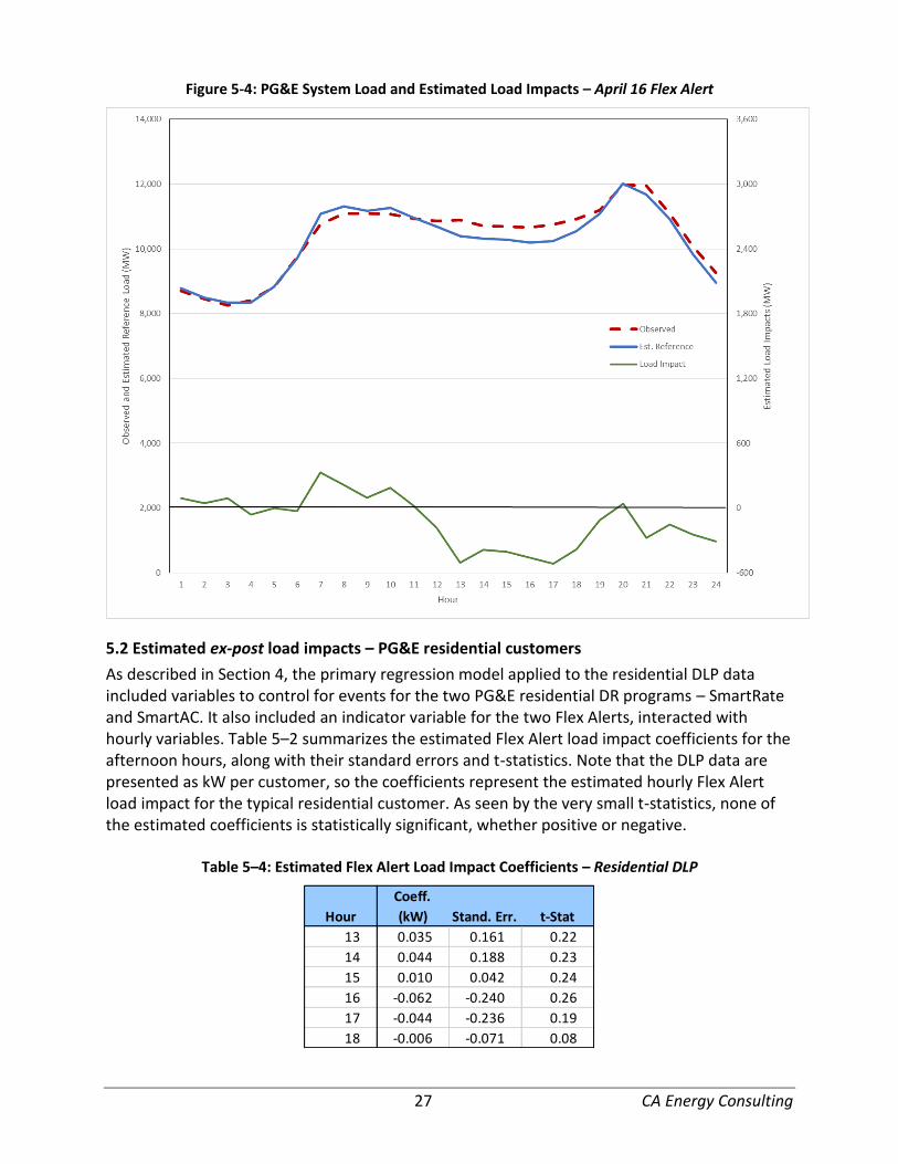
Figure 5-4: PG&E System Load and Estimated Load Impacts – April 16 Flex Alert ....................... 27

Figure 5–5 DLP Loads and Estimated Load Impacts – Average Flex Alert .................................... 28

Figure 5–6: DLP Loads and Estimated Load Impacts – April 16 Event .......................................... 29

1 CA Energy Consulting

ABSTRACT

This report describes the results of a load impact evaluation of California’s Flex Alert program for Program Year 2013. Flex Alerts are issued by the California Independent System Operator (CAISO) in cases of potential electrical emergencies (i.e., operating reserves falling below a critical level) or transmission emergencies (i.e., overloaded transmission lines). Flex Alerts are voluntary calls for consumers to reduce usage during afternoon hours (e.g., 12 p.m. until 6 p.m.) on the day of the alert. The primary objective of the evaluation was to estimate the extent to which consumers reduced their energy consumption during Flex Alerts. Two Flex Alerts were called in the summer of 2013, on July 1 and 2, both targeted only to Northern California, which contains Pacific Gas and Electric’s (PG&E’s) service territory. A localized Flex Alert was called on April 16, 2013 for the San Jose area, particularly Santa Clara and Silicon Valley, after vandalism severely damaged transformers at a substation in the area. As a result of the geographical targeting of these events, this study only involved analysis of system load and residential dynamic load profile (DLP) data for PG&E. The approach agreed upon by the Demand Response Measurement and Evaluation Committee (DRMEC) stakeholders for this project was to conduct a “top-down” statistical analysis of PG&E system load data, where the analysis was designed to control for the effects of factors such as weather conditions, day of week, and typical hourly load patterns, as well as the occurrence of any of PG&E’s demand response (DR) programs on Flex Alert days. The study’s primary finding is that no statistically significant (i.e., measureable) reductions in energy consumption attributable to the Flex Alerts could be found. Two primary factors likely contributed to these findings:

The April Flex Alert day applied to only Santa Clara and the Silicon Valley area, some of which is not in PG&E’s service territory, and only data for PG&E’s entire service area were available for the study.

Both of the July Flex Alert days coincided with event days for nearly every PG&E demand response program, which limited the ability to isolate any load reductions due to Flex Alert from the load reductions caused by the DR programs, given the inherent variability in the system load data. In addition, the fact that the DR programs were called on the same days as the Flex Alerts also likely reduced the potential for Flex Alert effects, since many of the consumers who have both the greatest capability and willingness to reduce load on specific days are those that have enrolled in utility DR programs, and they were already reducing load through those programs on the Flex Alert days.


EXECUTIVE SUMMARY

This report describes the results of a load impact evaluation of California’s Flex Alert program for Program Year 2013. Flex Alerts are issued by the California Independent System Operator (CAISO) in cases of potential electrical emergencies (i.e., operating reserves falling below a critical level) or transmission emergencies (i.e., overloaded transmission lines). Flex Alerts are voluntary calls for consumers to reduce usage during afternoon hours (e.g., 12 p.m. until 6 p.m.) on the day of the alert. Primary Research Objective

The primary objective of this evaluation was to estimate the extent to which consumers are found to have reduced their energy consumption during Flex Alerts. Two Flex Alerts were called in the summer of 2013, on July 1 and 2, both targeted only to Northern California, which contains Pacific Gas and Electric’s (PG&E’s) service territory. A localized Flex Alert was called on April 16, 2013 for the San Jose area, particularly Santa Clara and Silicon Valley, after vandalism severely damaged transformers at a substation in the area. As a result of the geographical targeting of these events, this study only involved analysis of system load and residential dynamic load profile (DLP) data for PG&E. Research Approach

The approach agreed upon by the Demand Response Measurement and Evaluation Committee (DRMEC) stakeholders for this project was to conduct a “top-down” statistical analysis of PG&E system load data, where the analysis is designed to control for the effects of factors such as weather conditions, day of week, and typical hourly load patterns, as well as the occurrence of any of PG&E’s demand response (DR) programs on Flex Alert days. The analysis seeks to use the load data on non-Flex Alert days to estimate a “reference load” on Flex Alert days that is designed to represent what PG&E’s system load would have been had the Flex Alert not been called. Estimates of the effects of the Flex Alerts are then obtained by subtracting the observed load on the Flex Alert days from the estimated reference load.1 Complicating this 2013 evaluation of the Flex Alert program is the fact that PG&E called events for nearly all of its DR programs on the same days that the two main Flex Alerts were called. This confluence of DR events and Flex Alerts complicates the problem of isolating the effects of Flex Alerts from the effects of the other programs.

1 In practice, we accounted for the effects of PG&E’s DR programs by adding estimates of their hourly load impacts to the observed system loads on the DR event days, thus producing adjusted system loads, from which Flex Alert load impacts were estimated. That is, Flex Alert load impacts were calculated as the difference between estimated reference loads (which are based on analysis of the adjusted system load data) and the observed system load on Flex Alert days.


Primary Findings

The primary finding from this study is that no statistically significant (i.e., measurable) reductions in energy consumption could be attributed to the Flex Alerts. The individual hourly load impact estimates range widely, from one value representing a 220 MW (1.2 percent) load reduction to another representing a 600 MW load increase. None of the estimates can be judged to be significantly different from zero, due to uncertainty around the estimated values. The averages of the hourly point estimates, for the afternoon hours of 12 noon to 6 p.m., on July 1 are 17 MW (not statistically significant) and -175 MW (not statistically significant) on July 2.2 The latter result indicates a load increase relative to the load level that would have occurred in the absence of the Flex Alert. Because load impacts are estimated rather than directly observed, there is a wide range of uncertainty associated with each of these estimates. This uncertainty is due to the fact that system load varies for many reasons (e.g., weather conditions, unexpected operational changes by large industrial customers, vacation schedules of residential customers), only some of which can be accounted for in our study from the available data. The analysis of the April Flex Alert day found load increases in the range of 400 to 500 MW.3 These findings are consistent with previous Flex Alert evaluations (see Section 3) conducted on a statewide-basis in 2008 and with the Peak Time Rebate (PTR) evaluations done for San Diego Gas & Electric (SDG&E) and Southern California Edison (SCE) in 2012. Two primary factors likely contributed to these findings:


Both of the July Flex Alert days coincided with event days for nearly every PG&E demand response program, which limited our ability to isolate any load reductions due to Flex Alert from the load reductions caused by the DR programs, given the inherent variability in the system load data.4

2 These estimates are incremental to the 300 to 500 MW load impacts from PG&E’s DR programs that were also called on the two Flex Alert days, since those impacts were accounted for in the analysis, as described in the previous footnote. 3 These estimated load increases are likely due to omitted variable bias (i.e., due to factors associated with the Flex Alert days, such as hotter than normal weather, that are not fully accounted for in the regression model), and not because customers responded to the Flex Alerts by increasing their usage levels. 4 In addition to complicating the analysis of Flex Alert load impacts, the fact that the DR programs were called on the same days as the Flex Alerts also likely reduced the potential for Flex Alert effects. This is the case because many of the very consumers who have both the greatest capability and willingness to reduce load on specific days are those that have enrolled in utility DR programs, and they were already reducing load through those programs on the Flex Alert days.


1. INTRODUCTION AND PURPOSE OF STUDY

This report describes the results of a load impact evaluation of California’s Flex Alert program for Program Year 2013. Flex Alerts are issued by the California Independent System Operator (CAISO) in cases of potential electrical emergencies (i.e., operating reserves falling below a critical level) or transmission emergencies (i.e., overloaded transmission lines). Flex Alerts are voluntary calls for consumers to reduce usage during afternoon hours (e.g., 12 p.m. until 6 p.m.), where announcements are made through public media, press releases, utility websites, and other outlets.5 The primary objectives of this evaluation are the following:

1. To estimate the ex-post load impacts of the Flex Alert program in 2013, using methods that conform to the Load Impact Protocols; and

2. To develop Flex Alert program load impact estimates for the residential sector, using PG&E dynamic load profile data, and for all sectors combined using PG&E system load data.

These goals involve estimating hourly load impacts for each Flex Alert. They also nominally involve reporting estimated load impacts for each hour of the average event day, for the average customer and all customers in aggregate. The DR protocols generally call for also reporting load impacts for the average event by customer type (e.g., business types) and for each CAISO local capacity area (LCA). However, due to the planned high-level analysis using system-level load data for most of this study, results for PG&E are for the most part reported at that level. The report is organized as follows. Section 2 describes the Flex Alert program and illustrates PG&E’s system load and weather conditions on the Flex Alert days; Section 3 provides background from previous Flex Alert evaluations; Section 4 describes the analysis methods used in the study; Section 5 contains the ex post load impact results; Section 6 provides conclusions and recommendations; and Appendix A describes the model validation process.

2. DESCRIPTION OF RESOURCES COVERED IN THE STUDY

2.1 Program Description

Flex Alerts are issued by the CAISO in cases of potential electrical emergencies (i.e., operating reserves falling below a critical level) or transmission emergencies (i.e., overloaded transmission lines). Flex Alerts are voluntary calls for consumers to reduce usage during afternoon hours (e.g., 12 p.m. until 6 p.m.) on the day of the alert. Two Flex Alert events were called in the summer of 2013, on July 1 and 2, both targeted only to Northern California, which contains PG&E’s service territory. A localized Flex Alert event was called on April 16, 2013 for the San Jose area, particularly Santa Clara and Silicon Valley, after vandalism severely damaged transformers at a substation in the area. As a result of the geographical targeting of these

5 While the focus is typically on summer afternoon hours, CAISO maintains flexibility to request reductions in other hours as conditions may indicate.


events, this study only involves analysis of system load and dynamic load profile data for PG&E for the Flex Alert evaluation.

2.2 Event Summary

A summary of the events subject to evaluation in this study is as follows:

April 16, 2013 – Flex Alert called for Santa Clara and Silicon Valley area only

July 1 and 2, 2013 – Flex Alert events called for Northern California

2.3 Features of DR events and Flex Alerts

Before turning to a description of analysis methods and the study results, we first review the system load and weather conditions on the Flex Alert days and selected comparable days, as well as estimates of the load impacts of PG&E’s DR programs, most of which were called on the same days. Figure 2–1 shows the observed PG&E system load profiles for the two Flex Alert days (dashed lines near the top of the graph) and other selected high-load days. The maximum system load appears to have occurred on July 3 in hour 17, at approximately 19,620 MW, closely followed by the loads on the two previous days, on which Flex Alerts were called. Another group of moderately high-load days reached approximately 17,000 MW, including September 9, on which many DR programs were called. The shaded area in the graph indicates the important afternoon hours of 12 p.m. to 6 p.m. in which loads tend to be highest and load reductions are most valuable. There appears to be a “dip” in usage beginning in hour 15 on both of the Flex Alert days, which is in contrast to the smoother load shape on the two other hot days. However, as shown below, a number of PG&E DR events were called on those days as well, which makes it difficult to use Figure 2–1 to illustrate whether customers reduced load due to Flex Alert.


Figure 2–1: PG&E System Load Profiles on Flex Alert and Comparable Days

Figure 2–2 shows the average estimated event-hour load impacts for each of PG&E’s DR program events that were called through September 2013, as indicated in PG&E’s post-event operational reporting.6 The figure shows that most of the programs were called on the two Flex Alert days of July 1 and 2, as well as on September 9. A full BIP event was also called on July 2. Average event-hour estimated load impacts are approximately 300 MW on July 1 and September 9, and more than 500 MW on July 2. Average event-hour load impacts are less than 100 MW on most other DR event-days. Note that no DR program events were called on the April 16 Flex Alert day.

6 These load impacts are calculated immediately after the events occur, using program baselines, and thus differ from the ex-post load impacts that are estimated in the program load impact evaluations that are filed on April 1. However, the two sources of load impact estimates are typically reasonably close.


Figure 2–2: Average Event-Hour DR Load Impacts by Program and Event-Day

Figure 2–3 shows how the overall average estimated event-hour load impacts shown in Figure 2–2 are spread across the key afternoon hours on the two Flex Alert days and two similar days. The greatest load impacts are estimated to occur in hours-ending 16 through 18 (3 p.m. to 6 p.m.), falling off somewhat in hour 19. These are the primary hours in which events were called for the major DR programs.


Figure 2–3: Estimated Hourly DR Load Impacts for Selected Days

Figure 2–4 illustrates the effect that the estimated DR program load impacts shown in Figure 2–3 are likely to have had on the PG&E system load. The dashed lines for the two Flex Alert days, as well as for July 3, are constructed by adding the estimated hourly load impacts shown in Figure 2–3 back into the observed system loads to produce an estimate of what the system loads would have been if the DR programs had not been called.7 The adjusted loads suggest that had the DR program events not been called, the system peak day would have actually occurred on July 2 rather than July 3.

7 Note that the post-event operational load impacts include values only for program event hours, which typically differ across programs. They thus do not account for either load reductions beginning immediately prior to the events, or continuing reductions or rebound effects in hours immediately following the event windows. These factors are likely the cause of the spiked shape of the adjusted loads in Figure 2–4.


Figure 2–4: PG&E System Loads Adjusted for DR Load Impacts

The following two figures illustrate the link between weather conditions and system load levels, and the nature of the Flex Alert days. Figure 2–5 shows system-wide temperature profiles for selected days, showing that the two Flex Alert days on July 1 and 2 were among the four hottest days of the summer. Another group of somewhat less hot days are shown below the top four, including September 9, on which a number of DR events were called.


Figure 2–5: Temperature Profiles on Flex Alert and Comparable Days

Figure 2–6 combines the load and temperature information shown in the figures above to illustrate the relationship between the temperatures and system loads. This provides an initial examination of whether the load levels on Flex Alert days are lower than loads on non-Flex Alert days, controlling for the effect of temperature on load levels. The figure charts the relationships between daily observations on temperature and average hourly usage in hours 13 to 18. Observations for the two Flex Alert days are shown by the two larger data points toward the top right portion of the graphs. Two trend lines are also shown—a linear trend and a quadratic trend fit, the latter suggesting a possible non-linear relationship. A clear direct relationship may be seen between daily afternoon temperatures and loads. The observations for both the two Flex Alert days and the two other hottest days lie above both trend lines, indicating that average hourly usage on those days is actually higher than one would expect given the temperatures on those days and the relationship between load levels and temperatures across other summer days.8 Note also that the values for the Flex Alert days in Figure 2–6 represent observed loads, which reflect the reduced loads resulting from PG&E’s DR programs called on those days. Adding the DR load impacts back into the observed loads (to

8 The higher than average loads on the hottest days suggest a non-linear relationship between afternoon loads and temperatures. In fact, our preferred regression model for which results are shown in Section 5 includes a squared value of a daily weather variable in an attempt to capture potential non-linearities.


improve comparability across observations) would place the Flex Alert data points even further above the load level implied by the load-temperature relationship across other days. These observations suggest that any additional Flex Alert usage reductions, beyond those already induced by the DR programs, are likely to be relatively small and difficult to estimate.

Figure 2–6: Average Hourly System Load vs. Average Hourly Temperature – Hours 13 to 18

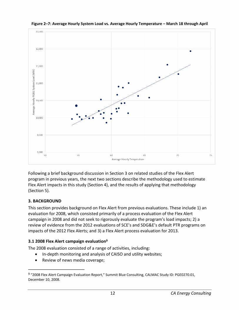
We conducted a similar comparison of average system loads and temperatures for the April 16 Flex Alert day. Figure 2–7 shows the relationship between daily observations on average hourly system load and temperatures for the weekdays between March 18 and April 30. The large point near the lower left corner represents the April 16 Flex Alert day. Similar to the summer case shown above, the average load level is above the load levels from days with similar temperatures, suggesting again that the statistical models are not likely to estimate significant usage reductions on the Flex Alert day.


Figure 2–7: Average Hourly System Load vs. Average Hourly Temperature – March 18 through April

Following a brief background discussion in Section 3 on related studies of the Flex Alert program in previous years, the next two sections describe the methodology used to estimate Flex Alert impacts in this study (Section 4), and the results of applying that methodology (Section 5).

3. BACKGROUND

This section provides background on Flex Alert from previous evaluations. These include 1) an evaluation for 2008, which consisted primarily of a process evaluation of the Flex Alert campaign in 2008 and did not seek to rigorously evaluate the program’s load impacts; 2) a review of evidence from the 2012 evaluations of SCE’s and SDG&E’s default PTR programs on impacts of the 2012 Flex Alerts; and 3) a Flex Alert process evaluation for 2013.

3.1 2008 Flex Alert campaign evaluation9

The 2008 evaluation consisted of a range of activities, including:

In-depth monitoring and analysis of CAISO and utility websites;

Review of news media coverage;

9 “2008 Flex Alert Campaign Evaluation Report,” Summit Blue Consulting, CALMAC Study ID: PGE0270.01, December 10, 2008.


Process interviews;

Focus groups;

A post-event survey following the July 2008 three-day Flex Alert; and

Estimation of Flex Alert demand impacts through a combination of engineering simulation and inferences regarding self-reported customer actions from the post-event survey.

Key findings of the study included the following:

Improvement in the consistency of messages in CAISO and utility communications relative to 2007, but with some room for improvement;

There was significant and reasonably accurate media coverage (e.g., using correct Flex Alert terminology), which declined somewhat from the first Flex Alert on July 8, to the last one on July 10;

The focus groups found some awareness of Flex Alert, but it was generally characterized at “saving, or conserving energy,” without an apparent understanding of the limited and timely nature of Flex Alerts;

The post-event survey found fairly wide recollection (about 60 percent) of seeing some type of energy conservation alert or message in the past 10 days, with TV being cited most often. However, less than half of those who recalled a message understood that the conservation was needed at particular times of day, and fewer understood that it was especially needed on certain days. Just over half of those who recalled a message or alert reported taking conservation actions in response, which translates into 37 percent of respondents.

The “indirect” impact analysis consisted of engineering simulations of lighting and air conditioner behaviors, based on customers’ self-reported actions taken, from the post-event survey. The simulations produced estimated reductions in energy usage of approximately 222 to 282 MW for Flex Alert. No information was provided on the statistical significance of, or the uncertainties surrounding these estimates. That approach is in contrast to the statistical analysis conducted in this study, which uses observed load data on the Flex Alert days and other similar days to estimate Flex Alert impacts and provide evidence of uncertainty around the estimates.

3.2 Evidence from 2012 impact evaluations of SCE and SDG&E PTR programs

This section summarizes information from the 2012 load impact evaluations of SCE’s and SDG&E’s peak time rebate (PTR) programs that may shed light on the effect of the two Flex Alerts that were called in 2012. Nearly all SCE and SDG&E residential customers for whom smart meters had been installed and made operational were eligible for PTR credits in 2012, as well as a large number of SDG&E’s small commercial customers. SDG&E’s PTR evaluations covered both notified (Opt-in Alert) and non-notified residential and small commercial customers. SCE’s evaluation covered only notified residential customers, including those who opted in to receive notification and those who were defaulted into notification on the basis of email address availability.


3.2.1 Summary of PTR events and Flex Alerts

SDG&E called seven PTR events in 2012, two of which occurred on the two Flex Alert days of August 10 and August 14. SCE called six PTR events, one of which was on the same day as the August 10 Flex Alert day. However, the August 14 Flex Alert day was not called as an SCE PTR event. These different joint event patterns imply differences in how inferences might be made about what effects the Flex Alerts had on the energy usage of SCE’s and SDG&E’s residential and small commercial customers, as discussed below.

3.2.2 SCE PTR

The SCE PTR analysis was conducted for four groups of notified customers, which were defined by climate zone (inland or coastal) and notice type (whether the customer opted into PTR event notification, or was defaulted into it). The ex-post regression models included one set of explanatory variables to separately indicate each of the six PTR event days, and another set of variables to account for both Flex Alert days. Therefore, the estimated Flex Alert load impact is a combination of the incremental load response (in addition to the PTR effect) on August 10 and the stand-alone load response to the Flex Alert event on August 14. Figure 3–1 shows the estimated hourly Flex Alert percentage load impacts for each of the four customer groups, where we follow the convention that positive values correspond to event-hour load reductions. As seen in the graph, however, the majority of the values shown are negative, indicating usage increases on Flex Alert days. Of the 96 hourly estimates shown in the figure (24 values for each of the four groups), only one is positive and statistically significant, 10 are negative and statistically significant, and the remaining 85 values are not statistically significantly different from zero. Note that the estimated PTR load impact on August 10 averaged 7.8 percent (across all four customer groups) and was statistically significant. However, the estimates indicate that this response is entirely attributable to PTR. We conclude from these estimates that SCE’s PTR customers who received event notification did not respond to the Flex Alerts.


Figure 3–1: Estimated Flex Alert Percentage Load Impacts, SCE PTR for PY2012

3.2.3 SDG&E PTR

The load impact regressions used in the SDG&E PTR impact evaluation, like those for SCE, included separate event-day indicators for each PTR event. Since both Flex Alert days overlap with PTR events, it is not possible to directly estimate a separate Flex Alert impact on the part of the PTR customers. The only way to potentially infer an incremental Flex Alert effect is to compare the estimated load impacts for the joint PTR/Flex Alert days to the impacts on the other PTR event days to see if any differences are apparent.

Residential PTR

The 2012 load impact evaluation of SDG&E’s residential PTR program analyzed data and reported results for a variety of customer groups and subgroups, including the following:10

Customers who opted to receive electronic notification of PTR events (Opt-in Alert);

Customers who participated in the San Diego Energy Challenge (SDEC);

Customers with in-home displays (IHD);

Customers who signed up for MyAccount; and

The remaining population of non-Alert, non-SDEC, and non-MyAccount customers. The primary findings of the residential PTR evaluation may be summarized as follows:

10 “2012 Load Impact Evaluation of San Diego Gas & Electric’s Residential Peak Time Rebate Program,” SDG0266.01, CA Energy Consulting, April 1, 2013.


No statistically significant usage reductions could be found for the non-Alert customer groups, including those who signed up for MyAccount (for most events, usage was found to increase during the event window).

Small but statistically significant usage reductions were found for the average SDEC, IHD, and Opt-in Alert customers. However, estimated reductions on the two Flex Alert days were no greater than those on other event days. The typical pattern is that usage reductions on August 10 were at or slightly below the average across all events, while those on August 14 were below average.11

Small commercial PTR

A separate evaluation of SDG&E’s small commercial PTR program reported similar findings of no significant usage reductions for non-notified customers, and smaller and less consistent reductions for Opt-in Alert commercial customers than those for residential customers, again with no evidence of greater reductions on the two Flex Alert days.12

Conclusions from SDG&E studies

We conclude from these two studies that there is no evidence that SDG&E’s residential or small commercial customers responded any differently on the two joint PTR and Flex Alert days than they did on the other PTR event days.

11 Average event-period temperatures were nearly the same on August 10 and 14, although the 10

th was the third

of four increasingly hot days, while the 14th

followed two days of higher but declining temperatures. 12 See “2012 Load Impact Evaluation of SDG&E’s Small Commercial PTR Program,” SDG0267, Enernoc Utility Solutions, March 27, 2013.


3.3 2013 Flex Alert process evaluation

A Flex Alert process evaluation was undertaken for 2013.13 The primary activities of the evaluation included the following:

A general awareness survey;

In-depth process interviews with key stakeholders;

Investigation of 2013 media coverage, including website traffic;

Survey of Flex Alert Network organizations; and

Document and website review. Unfortunately, the project was initiated in the fall of 2013, which precluded the ability to conduct a post-event survey immediately following the August Flex Alerts. Among the key findings of the process evaluation that may be relevant to this study are the following:

The bulk of the Flex Alert media expenditures focused on Southern California due to concerns about capacity availability as a result of the SONGS unavailability, while the only Flex Alerts turned out to be called for Northern California only;

Awareness of the term Flex Alert was relatively high, at approximately 60 percent, although awareness was appreciably higher in Southern California, particularly when awareness was restricted to messages seen in 2013, presumably due to the more intense media campaign there;

There is likely confusion between Flex Alert messaging and requests regarding reductions through utility DR programs (e.g., two-thirds of respondents rated bill credits as an important reason for responding to requests, whereas bill credits are not an element of Flex Alert);

Approximately half of respondents correctly identified Flex Alerts as applying to a limited number of summer days, and to afternoon hours;

A majority of responders recalled appropriate actions such as postponing lighting and major appliance use, and setting thermostats higher, with the highest recollections among those who received messages through TV or radio.

4. STUDY METHODOLOGY

4.1 Overview

In contrast to typical utility-sponsored demand response (DR) programs, Flex Alert is a voluntary educational and emergency alert program in which the CAISO initiates alerts and issues public requests for all consumers (sometimes differentiated by geographical zones within the state) to reduce usage through the afternoon peak hours. Thus, in essence, all electricity consumers in the state (or the relevant region of the state) are potential participants. However, they may not be aware of the events, and they have no financial incentive to reduce usage; the conservation request is only voluntary.

13 “Process Evaluation of the Statewide Flex Alert Program in 2013,” Draft Interim Report, Research Into Action, January 23, 2014.


The analysis approach agreed upon by the stakeholders in this project for evaluating the usage reductions provided by all customers on Flex Alert days, consists primarily of a top-down analysis of PG&E’s system-level load data, with a supplemental analysis of PG&E’s dynamic load profile (DLP) data for residential customers.14 The analysis controls for the effects of factors such as weather conditions, day of week, and typical hourly load patterns, as well as the occurrence of events for PG&E’s demand response (DR). Essentially, the analysis seeks to use the load data on non-Flex Alert days to estimate a reference load on Flex Alert days that is designed to represent PG&E’s system load (or its residential DLP) as it would have occurred had the Flex Alerts not been called. Estimates of the effects of the Flex Alerts are then obtained by subtracting the observed load on the Flex Alert days from the estimated reference loads. Complicating this evaluation of Flex Alert impacts is the fact that PG&E called events for nearly all of its DR programs on the same days for which the two main Flex Alerts were called.

In an ideal experimental setting, we would observe a mixture of similar hot days on which either DR program events or Flex Alerts are called, along with some days on which both are called. In such a setting, a statistical analysis could isolate the effects of Flex Alerts from those of the DR programs. Unfortunately, in the real world, only a limited number of hotter than normal days occur, and Flex Alerts and DR programs are called for economic and reliability reasons rather than as part of an experimental design. As illustrated in Figure 2–2, the two July Flex Alerts occurred on the same days on which most DR programs were called. This factor complicates attempts to isolate the effects of the Flex Alerts.15 The following sub-section provides details on our approach for estimating the Flex Alert load impacts.

4.2 Description of Methods

For the overall Flex Alert evaluation, we applied a top-down regression analysis to hourly PG&E system load data for the summer months, along with information on the events for all other DR programs that were called by PG&E during the summer. A separate analysis of system load data for March through May was undertaken to estimate the effects of the localized Flex Alert event in April, 2013. To estimate Flex Alert load impacts for PG&E’s residential customers, we analyzed PG&E DLP load data and included information on all residential DR program events.

Our approach to estimating load impacts may be described through the following equation:

Flex Alert Load Impact = Reference Load – Adjusted Observed Load

The steps used to develop this equation are as follows:

14 An alternative approach might have involved an analysis of load data for samples drawn from all classes of customers. However, the sampling approach that would be needed to account for DR program enrollments (so that we properly account for the effects of the PG&E DR program events) was judged to be too costly and time consuming to implement. 15 In addition to complicating the analysis of Flex Alert load impacts, the fact that the DR programs were called on the same days as the Flex Alerts also likely reduces the potential for Flex Alert effects. This may be the case because many of the very consumers who have both the greatest capability and willingness to reduce load on specific days are those that have enrolled in utility DR programs, and they were already reducing load through those programs on the Flex Alert days.


1. “Adjusted Observed Load” is calculated by adding the DR program load impacts to the observed PG&E system load. We use the load impact estimates from the post-event program settlements to complete this step.

2. The “Reference Load” represents the PG&E system load that would have occurred in the absence of the Flex Alert (and all other DR program events). It is estimated using a statistical model (described in detail below) that accounts for the effects of weather effects and typical usage patterns (e.g., usage levels tend to vary across hours of the day or days of the week).

3. The “Flex Alert Load Impact” is the difference between the Reference Load and the Adjusted Observed Load. This is the estimated effect of the Flex Alert on system load.

The equation and steps above provide a conceptual description of the method used to estimate Flex Alert load impacts. In practice, the load impacts are directly estimated using the statistical model described in the next sub-section.16

4.2.1 Analysis approach

The basic estimating equation for the Flex Alert analysis takes on a form similar to the equations used in previous DR evaluations, except that the load data represent hourly observations of system loads, rather than customer-level or average customer loads within a program. In addition, the actual loads are adjusted by adding estimated hourly DR load impacts to the observed loads on days when DR events were called. The model is shown below, with each term described in the following table:

t

i

titi

FRI

i

i

titi

MON

i

i

ti

h

i

i

ti

MONTH

i

i i i

t

DT

itti

Wth

itti

Flex

it

ehFRIbhMONbhb

MONTHbDTbWthhbFlexhbaQ

)()()(

)()()()(

24

2

,,

24

2

,,

24

2

,

8

7

,

24

1

24

1

5

2

,,

16 Because load impacts are estimated rather than directly observed, there is a range of uncertainty around the estimates (the “standard error”) that can be used to determine whether the estimated load impact is statistically significantly different from zero. The uncertainty is caused by the fact that PG&E system load can vary for many reasons, while our statistical model can only account for comparatively few factors. For example, we can incorporate the effect of changing weather conditions, but not the varying production schedules of the many electricity-intensive industrial customers in PG&E’s service territory.


Variable Name / Term Variable / Term Description

Qt the hourly usage in time period t for the PG&E system load, adjusted by adding estimated hourly DR load impacts on relevant event days

The various b’s the estimated parameters

hi,t an indicator variable for hour i

Flext an indicator variable for Flex Alert days

Wtht the weather conditions during hour t17

DTj,t indicator variables for each day of the week

MONTHi,t a series of indicator variables for each month

MONi,t an indicator variable for Mondays

FRIi,t an indicator variable for Fridays

et the error term

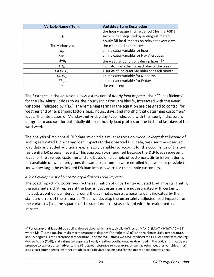
The first term in the equation allows estimation of hourly load impacts (the bi

Flex coefficients) for the Flex Alerts. It does so via the hourly indicator variables hi,t interacted with the event variables (indicated by Flext). The remaining terms in the equation are designed to control for weather and other periodic factors (e.g., hours, days, and months) that determine customers’ loads. The interaction of Monday and Friday day-type indicators with the hourly indicators is designed to account for potentially different hourly load profiles on the first and last days of the workweek. The analysis of residential DLP data involved a similar regression model, except that instead of adding estimated DR program load impacts to the observed DLP data, we used the observed load data and added additional explanatory variables to account for the occurrence of the two residential DR program events. This approach was required because the DLP loads represent loads for the average customer and are based on a sample of customers. Since information is not available on which programs the sample customers were enrolled in, it was not possible to know how large the estimated DR load impacts were for the sample customers.

4.2.2 Development of Uncertainty-Adjusted Load Impacts

The Load Impact Protocols require the estimation of uncertainty-adjusted load impacts. That is, the parameters that represent the load impact estimates are not estimated with certainty. Instead, a confidence interval around the estimates exists, whose range is indicated by the standard errors of the estimates. Thus, we develop the uncertainty-adjusted load impacts from the variances (i.e., the squares of the standard errors) associated with the estimated load impacts.

17 For example, this could be cooling degree days, which are typically defined as MAX[0, (MaxT + MinT) / 2 – 65], where MaxT is the maximum daily temperature in degrees Fahrenheit, MinT is the minimum daily temperature, and 65 degrees is the reference temperature. In some evaluations we have replaced the CDD variable with cooling degree hours (CDH), and estimated separate hourly weather coefficients. As described in the text, in this study we propose to explore alternatives to the 65-degree reference temperature, as well as other weather variables. In all cases, customer-specific weather variables are calculated using data for the appropriate climate zone.


The uncertainty-adjusted scenarios are simulated under the assumption that each hour’s load impact is normally distributed with the mean equal to the estimated load impacts and the standard deviation equal to the square root of the variances of the errors around the estimates of the load impacts. Results for the 10th, 30th, 70th, and 90th percentile scenarios are generated from these distributions.

5. DETAILED STUDY FINDINGS

5.1 Estimated ex-post load impacts – PG&E system level

System-wide July events

This section reports findings on the estimated system-level load impacts on the two July Flex Alert days. Table 5–1 shows estimated load impact coefficients from the regression equations described in Section 4.2.1, for the key afternoon hours from 12 noon to 6 p.m. (negative values indicate load reductions). It also shows the standard errors associated with the coefficients, and the resulting t-statistics. Statistical significance of the coefficients is determined by the degree of uncertainty surrounding the estimated coefficient value. That uncertainty is reflected in the standard error of the coefficient, and the t-statistic, which is the ratio of the coefficient to its standard error. For an estimated coefficient to be judged statistically significantly different from zero at a 95 percent confidence level, the absolute value of its t-statistic needs to be greater than approximately 1.96.18 As is evident in the table, none of the Flex Alert load impact estimates, whether positive or negative, meet that criterion (e.g., their standard errors are generally at least as great, or greater than the coefficient estimate). The average across the six afternoon hours of the estimated coefficients are -17 MW (an average load reduction) on July 1, and 175 MW (an average load increase) on July 2.

Table 5–1: Estimated Flex Alert Load Impact Coefficients – PG&E System Load

Figure 5–1 illustrates the estimated load impact coefficients and their corresponding confidence intervals, based on the standard errors shown in Table 5–1. Most of the coefficients are positive (i.e., load increases), particularly for the July 2 Flex Alert, presumably reflecting higher loads due to the fact that the alerts were called on two of the hottest days of the

18 That is, a relatively high t-statistic implies that the uncertainty around a given estimated coefficient is relatively small, giving confidence that its true value is within the confidence interval defined by the standard errors. In contrast, the small t-statistics in Table 5–1 imply that relatively little confidence may be placed in the estimated load impact values (i.e., the true value of the load impact could be quite different from the estimate).

Hour

Coeff.

(MW)

Stand.

Err. T-Stat

Coeff.

(MW)

Stand.

Err. T-Stat

13 227 245 0.926 594 348 1.707

14 159 223 0.713 266 314 0.849

15 -208 211 -0.987 -136 300 -0.454

16 115 202 0.568 235 277 0.849

17 -174 187 -0.932 55 254 0.218

18 -223 189 -1.181 35 256 0.138

July 1 Flex Alert July 2 Flex Alert


summer. A few negative coefficients occur in afternoon or evening hours for the July 1 alert, but none are statistically significant.19

Figure 5–1: Estimated Hourly Flex Alert Load Impact Coefficients and Confidence Intervals

Tables 5–2 and 5–3 show the estimated hourly Flex Alert load impacts (positive values are load reductions), along with the estimated reference load, observed load plus DR impacts, and observed load in the usual Protocol table format, for the July 1 and July 2 Flex Alerts. The primary difference from the usual DR program evaluations is the inclusion of the column for “Observed Load + DR”, which is the form of the data actually used in estimation. The tables also show uncertainty ranges associated with the hourly estimated load impacts.

19 The model for which the results are shown included a squared weather variable to control for possible non-linear weather effects. The estimates for the equation without the squared term had higher positive coefficients and fewer negative coefficients.


Table 5–2: PG&E System Loads and Estimated Flex Alert Load Impacts – July 1

Uncertainty Adjusted Impact (MWh/hr) - Percentiles

10th%ile 30th%ile 50th%ile 70th%ile 90th%ile

1 11,428 11,716 11,716 -288 72 -422 -343 -288 -233 -153

2 10,885 10,993 10,993 -108 71 -254 -168 -108 -48 39

3 10,492 10,657 10,657 -165 70 -289 -215 -165 -114 -40

4 10,437 10,600 10,600 -163 69 -292 -216 -163 -110 -33

5 10,747 10,814 10,814 -67 69 -198 -120 -67 -13 64

6 11,284 11,232 11,232 52 68 -145 -28 52 133 249

7 12,126 12,288 12,288 -162 68 -449 -280 -162 -45 125

8 13,022 13,232 13,232 -210 71 -488 -324 -210 -96 69

9 14,001 14,226 14,226 -225 75 -499 -337 -225 -113 49

10 14,906 15,255 15,255 -349 79 -638 -467 -349 -230 -60

11 15,812 16,296 16,296 -484 83 -815 -620 -484 -349 -154

12 16,560 16,887 16,887 -328 86 -647 -458 -328 -197 -9

13 17,431 17,658 17,625 -227 89 -541 -355 -227 -98 87

14 18,238 18,397 18,363 -159 91 -444 -275 -159 -42 127

15 18,918 18,710 18,599 208 93 -62 97 208 318 478

16 19,273 19,388 19,040 -115 93 -375 -221 -115 -9 145

17 19,421 19,247 18,905 174 92 -65 76 174 272 413

18 19,269 19,046 18,700 223 91 -19 124 223 322 464

19 18,819 18,843 18,540 -25 89 -249 -116 -25 67 200

20 18,083 18,143 18,101 -60 86 -308 -162 -60 42 188

21 17,598 17,866 17,866 -269 82 -425 -333 -269 -205 -113

22 16,119 16,543 16,543 -424 79 -596 -495 -424 -354 -252

23 14,512 14,770 14,770 -257 77 -477 -347 -257 -168 -38

24 13,122 13,482 13,482 -360 76 -570 -446 -360 -274 -150


10th 30th 50th 70th 90th

Daily 362,502 366,289 364,731 -3,787 161.5 n/a n/a n/a n/a n/a

Change in

Energy

Use

(MWh)

Cooling

Degree

Hours

(Base 75o

F)

(3)

Observed

Load

(MWh/hr)

Hour

Ending

(1)

Estimated

Reference

Load

(MWh/hr)

(2)

Observed

Load + DR

(MWh/hr)

(1) - (2)

Estimated

Load

Impact

(MWh/hr)

Weighted

Average

Temp. (oF)

Observed

Event-Day

Energy Use

(MWh)

Reference

Energy

Use

(MWh)

Observed

(+DR)

Event-Day

Energy

Use

(MWh)


Table 5–3: PG&E System Loads and Estimated Flex Alert Load Impacts – July 2

Figures 5–2 and 5–3 illustrate the loads and estimated load impacts (right axis) shown in the above tables, for the July 1 and July 2 Flex Alerts respectively. As in the tables, load reductions are by convention shown as positive values (i.e., reflecting negative estimated load impact coefficients). Few of the hourly load impacts are positive in the hours prior to hour 18, particularly on July 2. The effect of adding the DR load impacts into the observed loads may be seen as the difference between the Adjusted Observed (+DR) and Observed lines.


10th%ile 30th%ile 50th%ile 70th%ile 90th%ile

1 11,891 12,502 12,502 -610 75 -733 -661 -610 -560 -488

2 11,345 11,850 11,850 -505 74 -634 -558 -505 -453 -376

3 10,946 11,478 11,478 -532 73 -647 -579 -532 -485 -417

4 10,825 11,353 11,353 -528 72 -652 -579 -528 -477 -404

5 11,128 11,612 11,612 -484 71 -616 -538 -484 -430 -352

6 11,710 12,017 12,017 -307 71 -514 -392 -307 -222 -100

7 12,437 12,953 12,953 -516 70 -831 -645 -516 -387 -201

8 13,243 14,096 14,096 -853 73 -1,173 -984 -853 -722 -533

9 14,217 14,982 14,982 -766 76 -1,109 -906 -766 -625 -423

10 15,179 15,919 15,919 -741 80 -1,114 -893 -741 -588 -367

11 16,112 16,922 16,922 -810 84 -1,253 -991 -810 -629 -367

12 16,904 17,584 17,584 -679 87 -1,125 -862 -679 -497 -233

13 17,854 18,449 18,449 -594 90 -1,041 -777 -594 -412 -148

14 18,795 19,062 19,062 -266 92 -668 -431 -266 -102 136

15 19,328 19,192 19,081 136 93 -249 -21 136 294 521

16 19,666 19,901 19,382 -235 93 -591 -381 -235 -90 120

17 19,624 19,679 19,144 -55 92 -381 -189 -55 78 270

18 19,154 19,190 18,657 -35 89 -364 -170 -35 99 293

19 18,675 18,549 18,099 126 86 -178 2 126 250 430

20 18,222 17,582 17,579 640 83 313 506 640 774 967

21 17,456 17,239 17,237 217 79 10 132 217 302 425

22 15,974 15,988 15,986 -14 76 -256 -113 -14 85 228

23 14,448 14,443 14,442 6 75 -283 -113 6 124 294

24 13,002 12,987 12,987 16 73 -246 -92 16 123 278


10th 30th 50th 70th 90th

Daily 368,137 375,528 373,374 -7,391 150.0 n/a n/a n/a n/a n/a

(1) - (2)

Estimated

Load

Impact

(MWh/hr)

Weighted

Average

Temp. (oF)

Reference

Energy

Use

(MWh)

Observed

(+DR)

Event-Day

Energy

Use

(MWh)

Change in

Energy

Use

(MWh)

Cooling

Degree

Hours

(Base 75o

F)

(3)

Observed

Load

(MWh/hr)

Observed

Event-Day

Energy Use

(MWh)

Hour

Ending

(1)

Estimated

Reference

Load

(MWh/hr)

(2)

Observed

Load + DR

(MWh/hr)


Figure 5–2: PG&E System Load and Estimated Load Impacts – July 1 Flex Alert


Figure 5–3: PG&E System Load and Estimated Load Impacts – July 2 Flex Alert

April regional event

We estimated regression models for the April 16 event using data for March through May, and including heating as well as the cooling variables present in the model used to estimate July Flex Alert load impacts. As with the July models, no significant usage reductions could be found. Instead, statistically significant load increases were found in the afternoon hours.20 Figure 5–4 illustrates the estimated hourly load impacts, observed loads, and adjusted reference loads for each hour of the April Flex Alert day.21 The wrong-signed load impacts are consistent with the data shown in Figure 2–7, showing that the Flex Alert did not lead to usage reductions in PG&E’s service territory.22

20 These estimated load increases are likely due to omitted variable bias (i.e., due to factors associated with the Flex Alert days, such as hotter than normal weather, that are not fully accounted for in the regression model), and not because customers responded to the Flex Alerts by increasing their usage levels. 21 By convention, load reductions are shown as positive values; i.e., the “load impact” line would lie above zero for usage reductions. 22 Recall that the event was targeted at a limited geographic area in the Silicon Valley. However, the available load data were for the entire PG&E system, and some of the targeted area may have been outside of the PG&E service area.


Figure 5-4: PG&E System Load and Estimated Load Impacts – April 16 Flex Alert

5.2 Estimated ex-post load impacts – PG&E residential customers

As described in Section 4, the primary regression model applied to the residential DLP data included variables to control for events for the two PG&E residential DR programs – SmartRate and SmartAC. It also included an indicator variable for the two Flex Alerts, interacted with hourly variables. Table 5–2 summarizes the estimated Flex Alert load impact coefficients for the afternoon hours, along with their standard errors and t-statistics. Note that the DLP data are presented as kW per customer, so the coefficients represent the estimated hourly Flex Alert load impact for the typical residential customer. As seen by the very small t-statistics, none of the estimated coefficients is statistically significant, whether positive or negative.

Table 5–4: Estimated Flex Alert Load Impact Coefficients – Residential DLP

Hour

Coeff.

(kW) Stand. Err. t-Stat

13 0.035 0.161 0.22

14 0.044 0.188 0.23

15 0.010 0.042 0.24

16 -0.062 -0.240 0.26

17 -0.044 -0.236 0.19

18 -0.006 -0.071 0.08


Figure 5–5 shows the estimated reference load, observed load and estimated load impacts for the average DLP customer, where the convention is that load reductions are shown as positive values. However, none are statistically significant.

Figure 5–5 DLP Loads and Estimated Load Impacts – Average Flex Alert

A regression model was also estimated for the April 16 event using residential DLP data. The estimated load impacts are generally wrong signed and, like the July results, not statistically significant in the important late morning and afternoon hours. The per-customer estimated reference load, observed load, and estimated load impacts are shown in Figure 5–6.


Figure 5–6: DLP Loads and Estimated Load Impacts – April 16 Event

6. CONCLUSIONS AND RECOMMENDATIONS

In this study, we attempted to estimate ex-post load impacts for the Flex Alert program operated by the CAISO. However, we could find no statistically significant load reductions on Flex Alert days. Two primary factors contributed to this finding:


Both of the July Flex Alert days coincided with event days for nearly every PG&E demand response program, which limited our ability to isolate any load reductions due to Flex Alert from the load reductions caused by the DR programs, and also likely limited the potential for Flex Alert load reductions because many of the customers who might otherwise have reduced usage were already doing so as part of the DR programs.

An examination of the actual hourly usage data at the PG&E system level indicated some evidence of afternoon usage reductions on Flex Alert days, but those apparent load reductions coincided with the timing of PG&E’s DR program events, suggesting that isolating any additional Flex Alert impacts would be challenging. In addition, even allowing for estimated DR load reductions, the average observed afternoon load levels during the July Flex Alert days appeared high after accounting for the hot temperatures on those dates.


These findings may be considered generally consistent with findings reported in the draft Flex Alert process evaluation for 2013, which found that the program was marketed more heavily in Southern California than Northern California in anticipation of potential capacity constraints in that area. As a result, residents in Northern California were generally found to be less aware of Flex Alert than those in the southern part of the state. Stakeholders interested in studying the effects of Flex Alert face somewhat of a dilemma compared to the case for the utilities’ DR programs. Those programs allow test events, for which participants receive compensation for load reductions, and data are available for the participants to allow evaluation of load impacts. For purposes of evaluation, it would be useful to have at least one Flex Alert day on which few or no other DR program events are called. However, if Flex Alerts are only called on days for which reliability is at risk, then the utilities likely feel a need to call their DR programs on those days as well.


APPENDIX A. MODEL VALIDATION

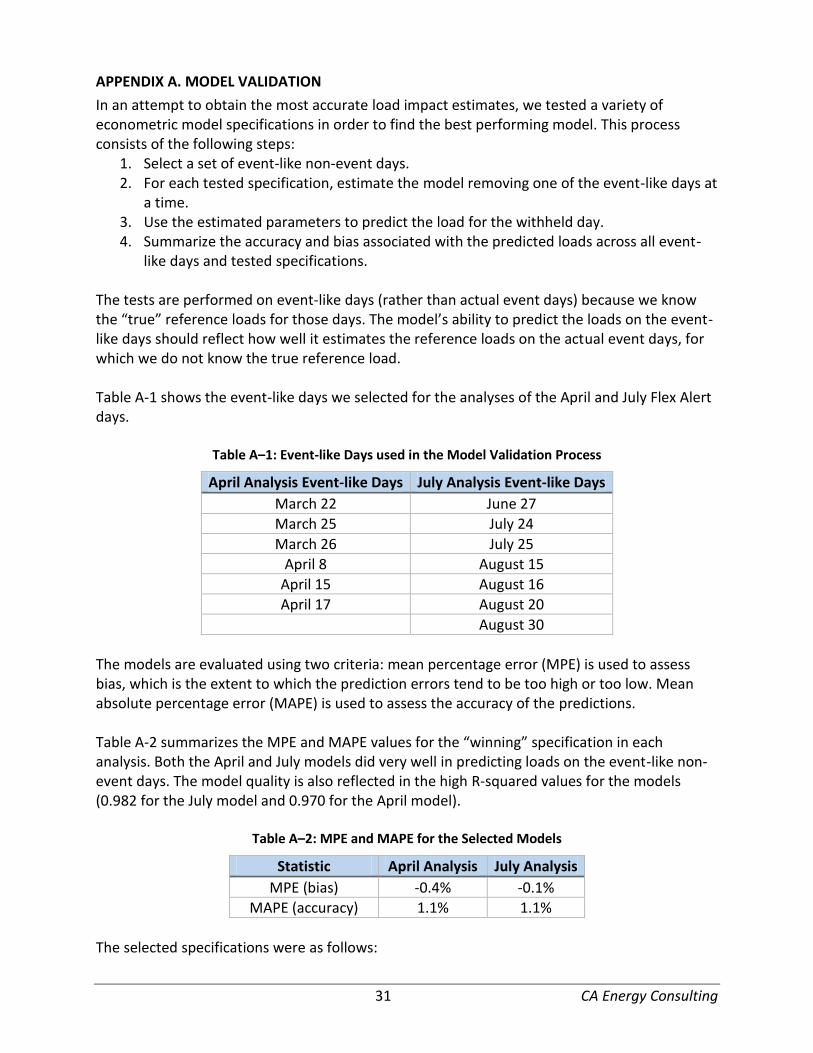
In an attempt to obtain the most accurate load impact estimates, we tested a variety of econometric model specifications in order to find the best performing model. This process consists of the following steps:

1. Select a set of event-like non-event days. 2. For each tested specification, estimate the model removing one of the event-like days at

a time. 3. Use the estimated parameters to predict the load for the withheld day. 4. Summarize the accuracy and bias associated with the predicted loads across all event-

like days and tested specifications. The tests are performed on event-like days (rather than actual event days) because we know the “true” reference loads for those days. The model’s ability to predict the loads on the event-like days should reflect how well it estimates the reference loads on the actual event days, for which we do not know the true reference load. Table A-1 shows the event-like days we selected for the analyses of the April and July Flex Alert days.

Table A–1: Event-like Days used in the Model Validation Process

April Analysis Event-like Days July Analysis Event-like Days

March 22 June 27

March 25 July 24

March 26 July 25

April 8 August 15

April 15 August 16

April 17 August 20

August 30

The models are evaluated using two criteria: mean percentage error (MPE) is used to assess bias, which is the extent to which the prediction errors tend to be too high or too low. Mean absolute percentage error (MAPE) is used to assess the accuracy of the predictions. Table A-2 summarizes the MPE and MAPE values for the “winning” specification in each analysis. Both the April and July models did very well in predicting loads on the event-like non-event days. The model quality is also reflected in the high R-squared values for the models (0.982 for the July model and 0.970 for the April model).

Table A–2: MPE and MAPE for the Selected Models

Statistic April Analysis July Analysis

MPE (bias) -0.4% -0.1%

MAPE (accuracy) 1.1% 1.1%

The selected specifications were as follows:


April model: 3-hour moving average of CDH55 and HDH55, 24-hour moving average of CDH55 and HDH55.

July model: current-hour heat index and the 24-hour moving average of the heat index.23

23 Heat index = c1 + c2T + c3R + c4TR + c5T

2 + c6R

2 + c7T

2R + c8TR

2 + c9T

2R

2 + c10T

3 + c11R

3 + c12T

3R + c13TR

3 + c14T

3R

2 +

c15T2R

3 + c16T

3R

3, where T = ambient dry-bulb temperature in degrees Fahrenheit and R = relative humidity (where

10 percent is expressed as “10”). The values for the various c’s may be found here: http://en.wikipedia.org/wiki/Heat_index.

http://en.wikipedia.org/wiki/Heat_index

Documents

2013 Impact Evaluation of California’s Flex Alert Demand … · Christensen Associates Energy Consulting, LLC 800 University Bay Drive, Suite 400 Madison, WI 53705 (608) 231-2266