2013 REPORT Prepared for: Creeks Division Prepared By scores for the seven core metrics are summed to provide a total score of between 0 and 70 for the study reach

SOUTHERN COASTAL SANTA BARBARA CREEKS AND ESTUARIES BIOASSESSMENT PROGRAM 2013 REPORT Prepared for: City of Santa Barbara, Creeks Division County of Santa Barbara, Project Clean Water Prepared By: www.ecologyconsultantsinc.com

Ecology Consultants, Inc.

Southern Coastal Santa Barbara Creeks and Estuaries Bioassessment Program Page 2 2013 Report

Executive Summary Introduction

This report summarizes the results of the 2013 Southern Coastal Santa Barbara Creeks and Estuaries Bioassessment Program, an effort funded by the City of Santa Barbara and County of Santa Barbara. The purpose of the Program is to assess and monitor the biological integrity of creeks and estuaries in the study area as they respond through time to natural and human influences. Ecology Consultants, Inc. (Ecology) prepared the report, and serves as the City’s and County’s consultant for the Program. This is the 14th year of the Program, which began in 2000.

The Program involves annual collection and analysis of benthic macroinvertebrate (BMI) samples and other pertinent physiochemical and biological data in 15 to 20 creek study reaches using U.S. Environmental Protection Agency (USEPA) endorsed rapid bioassessment techniques. BMI samples are analyzed in the laboratory to determine BMI abundance, composition, and diversity. Scores and classifications of biological integrity are determined for study streams using the Index of Biological Integrity (IBI) developed for study area creeks in 2009. The IBI yields a numeric score and classifies the biological integrity of a stream as Very Poor, Poor, Fair, Good, or Excellent based on the BMI community present in the stream. Seven “core BMI metrics” are calculated and used to determine the IBI score. Each core metric is highly sensitive to human disturbance, and collectively they represent different aspects of the BMI community including diversity, composition, and trophic group representation. By condensing complex biological data into an easily understood score and classification of biological integrity, the IBI serves as an effective tool for the City and County in monitoring the condition of local creeks, and evaluating the benefits or consequences of watershed management actions.

In 2011 the Program was expanded to include the estuaries of three local watersheds. Estuaries are open water bodies where a freshwater stream meets and mixes with saltwater from the ocean, creating brackish water conditions with salinities that change throughout the year depending on varying seasonal inputs from the stream and ocean tides. USEPA endorsed rapid bioassessment techniques for estuaries were used to collect BMI samples and other pertinent physiochemical and biological data. 6 estuaries were studied this year, as in 2012. The IBI cannot be used to assess the condition of local estuaries, which have very different physiochemical conditions (e.g., brackish water, substrate, water flow, etc.) and biological assemblages than do freshwater creeks. It is hoped that an IBI or similar tool to assess the condition of local estuaries can be developed in the future.

Study Area

The study area encompasses approximately 80 km of the southern Santa Barbara County coast from the Rincon Creek watershed at the Santa Barbara/Ventura County line west to Jalama Creek, which is just north of Point Conception. There are approximately 50 1st to 5th order coastal streams along this stretch of coast, all of which drain the southern face of the Santa Ynez Mountains. 52 different stream study reaches in 20 watersheds have been surveyed on one or more occasions from 2000 to 2013. 15 stream study reaches were surveyed this year, and 6 estuaries were surveyed.



Methods

Physiochemical and biological data for the study creeks and estuaries was gathered through a combination of methods including field surveys, laboratory analyses, spatial data analyses using geographic information system software, and review of United States Geological Survey (USGS) 7.5-minute quadrangle maps and recent aerial photographs. Core metrics were calculated and IBI scores and classifications of biological integrity were determined for the creek study reaches. A suite of BMI metrics was calculated for study estuaries, and evaluated for differences along disturbance and salinity gradients.

Results

Over the past 14 years, bioassessment data collected through the Program has provided a wealth of information regarding the physiochemical habitat conditions and biota (particularly the BMI community) present in local streams. The influences of natural physiochemical and climatic variability and human development on local stream communities have been extensively examined. The following general statements can be made based on the research completed thus far:

• Major episodic disturbances including extreme stream flows, drought conditions, and wildfires have been definitively shown to negatively impact stream communities, as evidenced by significantly lower IBI scores and loss or significant reduction of sensitive BMI and vertebrate taxa following such events. Local stream communities have proven to be resilient, typically showing dramatic recovery from extreme episodic disturbances in a year or two. However, some of the more sensitive species (e.g., rainbow trout) have yet to return to streams impacted by recent wildfires, and may require many years to fully recover.

• Negative impacts of human land use on local stream communities (particularly BMIs) have been documented with highly significant statistical test results. Degradation of stream communities (e.g., lower IBI scores and loss of sensitive species), as well as physiochemical habitat conditions, has increased linearly with increased watershed development, and urban development has been shown to have greater impacts on stream communities and habitat conditions than has agricultural development.

• Stream habitat restoration sites have shown improved habitat conditions, and in some cases slight improvements in the BMI community over time following restorative actions. Major improvements in stream community condition would likely require larger-scale, watershed-based restorative actions.

Over the past three years, a relatively limited data set has been compiled for local estuaries. Study sites have included the range available along a disturbance gradient, from “reference” sites that are fairly intact in form with little urbanization in their watersheds to “disturbed” sites that have been substantially altered in form and drain highly urbanized watersheds. Compared with streams, there appears to be less difference in BMI metrics between reference and disturbed estuaries. However, several BMI metrics, most of which are indices of sensitive and/or tolerant taxa, look promising as biological indicator metrics. More surveys are needed to further test, validate, and refine potential indicator metrics. Establishing 4 to 6 reliable indicator metrics will be the basis for developing a reliable IBI for local estuaries.



TABLE OF CONTENTS

Page I. INTRODUCTION .......................................................................................................... 5 II. STUDY AREA .............................................................................................................. 7 III. METHODS ............................................................................................................ 12

A. Field Surveys ............................................................................................. 12 B. Laboratory Analysis .................................................................................... 13 C. GIS Analyses ............................................................................................. 14 D. Review of Topographic Maps and Aerial Photographs ................................... 15 E. Study Reach Grouping ................................................................................ 15 F. Calculation of Core Metrics ......................................................................... 16 G. Core Metric Scoring Ranges ........................................................................ 17 H. IBI Classifications of Biological Integrity and Scoring Ranges ........................ 17 I. BMI Community Metrics for Estuaries .......................................................... 18

IV. RESULTS AND DISCUSSION .......................................................................................... 18 A. Physiochemical and Biological Data ............................................................. 18 B. IBI Scores and Classifications ..................................................................... 18 C. Rainfall and Peak Streamflow Effects on Creeks ........................................... 22 D. Estuaries ................................................................................................... 25

V. CLOSING ............................................................................................................ 32 VI. REFERENCES ............................................................................................................ 33 APPENDIX: DATA TABLES

FIGURES

Page Figure 1 Study Area .................................................................................................. 8 Figure 2 Gaviota Coast Study Reaches........................................................................ 9 Figure 3 Santa Barbara and Goleta Area Study Reaches ........................................... 10 Figure 4 Carpinteria Area Study Reaches .................................................................. 11 Figure 5 IBI Score by Year for 9 Study Reaches, 2002-2013 ...................................... 25 Figure 6 Selected BMI Parameter Means by Disturbance Class, 2012 and 2013 Estuaries (n=12) ........................................................................................ 30 Figure 7 Mean %BAIM and %COCO by Disturbance and Salinity ................................ 31

TABLES Page

Table 1 Study Reaches ............................................................................................. 7 Table 2 Core Metric Scoring Ranges ........................................................................ 17 Table 3 Classifications of Biological Integrity and Scoring Ranges.............................. 18 Table 4 Rainfall/Streamflow Data and Mean Physiochemical/BMI Parameter Values for 9 Study Reaches, Wet vs. Dry Years ...................................................... 23



I. Introduction

This report summarizes the results of the 2013 Southern Coastal Santa Barbara Creeks and Estuaries Bioassessment Program, an effort funded by the City of Santa Barbara and County of Santa Barbara. This is the 14th year of the Program, which began in 2000. Ecology Consultants, Inc. (Ecology) prepared this report, and serves as the City and County’s consultant for the Program. The purpose of the Program is to assess and monitor the “biological integrity” of study creeks and estuaries as they respond through time to natural and human influences. Karr and Dudley (1981) defined biological integrity as “the ability to support and maintain a balanced, integrated, adaptive community of organisms having a species composition, diversity, and functional organization comparable to that of natural habitat of the region.” (Miller et al., 1988). Bioassessment is the science of assessing the biological integrity of aquatic ecosystems by evaluating the biological assemblages (e.g., benthic macroinvertebrates, fish, amphibians, vegetation, etc.) that inhabit them. Because different taxa (i.e., species, genera, families, etc.) have varying habitat requirements and abilities to withstand water pollution and other forms of habitat disturbance, the presence or absence of particular taxa can serve as an indicator of the overall biological integrity a particular water body. On a broader level, measurements of the biological community relating to abundance, diversity, and trophic structure have proven to be reliable indicators of biological integrity in water bodies (Rosenberg and Resh, 1993, Barbour et al., 1999).

The Program involves annual collection and analysis of benthic macroinvertebrate (BMI) samples and other pertinent physiochemical and biological data in stream study reaches using U.S. Environmental Protection Agency (USEPA) endorsed rapid bioassessment methodology. Our sampling methodology has been consistent since 2000, and is very similar to that currently used for the California Surface Water Ambient Monitoring Program (SWAMP), the methods of which have varied over the years. BMI samples are analyzed in the laboratory to determine BMI abundance, composition, and diversity. Scores and classifications of biological integrity are determined for study streams using the BMI based Index of Biological Integrity (IBI) that was developed for study area streams in 2004, and updated in 2009. The IBI yields a numeric score and classifies the biological integrity of a given stream as Very Poor, Poor, Fair, Good, or Excellent based on the contents of the BMI sample collected from the stream. Seven “core metrics” are calculated and used to determine the IBI score. Each core metric is highly sensitive to human disturbance as determined through rigorous statistical analyses of data from local streams, and collectively they represent different aspects of BMI community structure including diversity, composition, and trophic group representation. The data set used to develop the IBI is robust, consisting of 10 years of surveys from a total of 190 stream sites that collectively are influenced by wide differences in physiochemical conditions and types and intensities of human disturbance. By condensing complex biological data into an easily understood score and classification of biological integrity, the IBI serves as an effective tool for the City and County in monitoring the condition of local creeks, and evaluating the benefits or consequences of watershed management actions. More discussion of the IBI and its development is provided in Southern Coastal Santa Barbara County Creeks Bioassessment Program, 2009 Report and Updated Index of Biological Integrity (Ecology Consultants, Inc., 2010).



In 2011 the Program was expanded to include local estuaries. Estuaries are open water bodies where a freshwater stream meets and mixes with saltwater from the ocean, creating brackish water conditions with salinities that change throughout the year depending on varying seasonal inputs from the stream and ocean. USEPA endorsed rapid bioassessment methods for estuaries were used to collect BMI samples and other pertinent physiochemical and biological data.

Over the past three years, a relatively limited data set has been compiled for local estuaries. Study sites have included the range available along a disturbance gradient, from “reference” sites that are fairly intact in form with little urbanization in their watersheds to “disturbed” sites that have been substantially altered in form and drain highly urbanized watersheds. As with last year, 6 estuaries were studied this year, including 3 “disturbed” and 3 “reference” estuaries.

The goal for last year was to compare the 3 disturbed estuaries to the 3 reference estuaries, and see whether there were notable differences in the BMI community and other biological parameters. BMI metrics with notable differences between these two groups of estuaries could have promise as core metrics for an estuarine IBI. Last year’s results indicate that there is generally less difference in BMI metrics between reference and disturbed estuaries compared to reference and disturbed creeks. Nonetheless, based on the limited data collected so far, several BMI metrics showed promise as ecological indicators in the estuaries, in particular two sensitivity/tolerance metrics that were developed in this study. This year’s effort provides additional data needed to further test, validate, and refine potential indicator metrics. Establishing 4 to 6 reliable indicator metrics will be the basis for developing a reliable IBI for local estuaries, which, at the current rate of study, is expected to take several years to accomplish.



II. Study Area

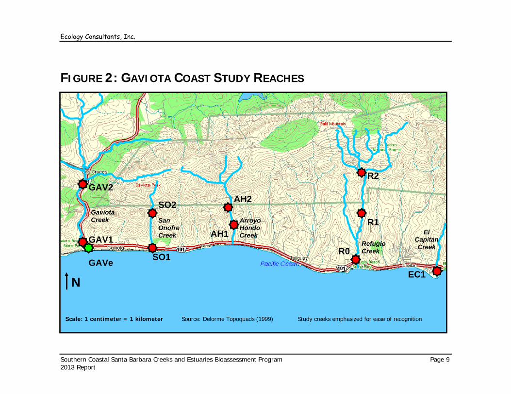
The study area encompasses approximately 80 km of the southern Santa Barbara County coast from the Rincon Creek watershed at the Santa Barbara/Ventura County line west to Jalama Creek, which is just north of Point Conception (see Figure 1). There are approximately 50 1st to 5th order coastal streams along this stretch of coast, all of which drain the southern face of the Santa Ynez Mountains. 52 different stream study reaches in 20 watersheds have been surveyed on one or more occasions from during the 14 years of the Program. 15 stream and 6 estuarine study reaches were surveyed this year. Table 1 lists this year’s study reaches and their locations. Figure 1 shows an overall map of the study area, and Figures 2, 3, and 4 provide more detailed maps and show the locations of the study reaches that have been surveyed over the years (except the Jalama Creek estuary).

Table 1: Study Reaches Study Reach Location Creek Study Reaches C1 Carpinteria Creek, 0.25 mi. downstream of Carpinteria Ave. C3 Gobernador Creek, approx. 0.25 mi. upstream of County detention basin SY1 Sycamore Creek just below Mason St. bridge SY3 Sycamore Creek 300m below Highway 192 crossing and Coyote/Sycamore confluence M1 Mission Creek at De la Guerra St. M2 Old Mission Creek at Bohnet Park M3 Mission Creek at upstream end of Rocky Nook Park M4 Rattlesnake Creek, approx. 0.5 mi. upstream of Las Canovas Rd. crossing AB1 Arroyo Burro at upstream end of Alan Rd. AB3 San Roque Creek, 0.25 mi. upstream of Foothill Rd. AB5 Mesa Creek at entrance to Arroyo Burro estuary SA2 San Antonio Creek just upstream of Highway 154 crossing SJ2 San Jose Creek, approx. 0.25 mi. upstream of Patterson Rd. crossing AH1 Arroyo Hondo, approx. 1 mi. upstream of U.S. 101. GAV1 Gaviota Creek at State Beach/Park, just below access rd./US 101 junction Estuary Study Reaches SYe Sycamore Creek estuary Me Mission Creek estuary ABe Arroyo Burro estuary Te Tecolote Creek estuary GAVe Gaviota Creek estuary Je Jalama Creek estuary



FIGURE 1: STUDY AREA

Source: Delorme Topoquads

N

Study Area



FIGURE 2: GAVIOTA COAST STUDY REACHES

SO2 AH1

San Onofre Creek

Arroyo Hondo

EC1

Refugio Creek

R2

R1 GAV1

Gaviota Creek

N

SO1

GAV2 AH2

Scale: 1 centimeter = 1 kilometer Source: Delorme Topoquads (1999) Study creeks emphasized for ease of recognition

San Onofre Creek

Arroyo Hondo Creek AH1

Refugio Creek

R2

R1

EC1

El Capitan Creek

SO2

GAVe R0


FIGURE 3: SANTA BARBARA AND GOLETA AREA STUDY REACHES


AT1

SJ1

SJ2

SJ3

AB2 AT2

N

San Jose Creek

Arroyo Burro

AB1 M1

M3

M2

Mission Creek SY1

Sycamore Creek

Scale: 1 centimeter = 1.5 kilometers Source: Delorme Topoquads (1999)

Atascadero Creek

San Antonio Creek

Maria Ygnacio Creek

MY1

SA1

Dos Pueblos Creek

DP1

T1

T2

Tecolote Creek

SJ4

MY2

MY3

SA2

M4

M6

M5

AB3

T3

AB7

AB5

AB6 SY2 SY3 AB4

ABe Me

SYe

Te



FIGURE 4: CARPINTERIA AREA STUDY REACHES

N

RIN1

Scale: 1 centimeter = 2 kilometers

C1 C2

Carpinteria Creek

Rincon Creek

C3 AP1 F1

Santa Monica

Creek Franklin

Creek

Source: Delorme Topoquads (1999) Study streams emphasized for ease of recognition

Arroyo Paredon

Creek

SM1 RIN0



III. Methods

Physiochemical and biological data for the creek and estuary study reaches was gathered through a combination of methods including field surveys, laboratory analyses, spatial data analyses using geographic information system (GIS) software, and review of United States Geological Survey (USGS) 7.5-minute quadrangle maps and recent aerial photographs. Biological parameters including core metrics and IBI scores (i.e., for creek study reaches) were calculated using the data. Further discussion of methods is provided below.

A. Field Surveys

1. Creeks

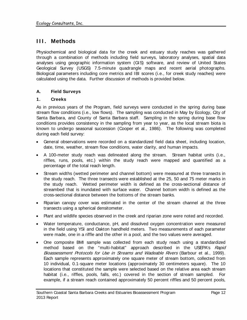
As in previous years of the Program, field surveys were conducted in the spring during base stream flow conditions (i.e., low flows). The sampling was conducted in May by Ecology, City of Santa Barbara, and County of Santa Barbara staff. Sampling in the spring during base flow conditions provides consistency in the sampling from year to year, as the local stream biota is known to undergo seasonal succession (Cooper et al., 1986). The following was completed during each field survey:

• General observations were recorded on a standardized field data sheet, including location, date, time, weather, stream flow conditions, water clarity, and human impacts.

• A 100-meter study reach was delineated along the stream. Stream habitat units (i.e., riffles, runs, pools, etc.) within the study reach were mapped and quantified as a percentage of the total reach length.

• Stream widths (wetted perimeter and channel bottom) were measured at three transects in the study reach. The three transects were established at the 25, 50 and 75 meter marks in the study reach. Wetted perimeter width is defined as the cross-sectional distance of streambed that is inundated with surface water. Channel bottom width is defined as the cross-sectional distance between the bottoms of the stream banks.

• Riparian canopy cover was estimated in the center of the stream channel at the three transects using a spherical densitometer.

• Plant and wildlife species observed in the creek and riparian zone were noted and recorded.

• Water temperature, conductance, pH, and dissolved oxygen concentration were measured in the field using YSI and Oakton handheld meters. Two measurements of each parameter were made, one in a riffle and the other in a pool, and the two values were averaged.

• One composite BMI sample was collected from each study reach using a standardized method based on the “multi-habitat” approach described in the USEPA’s Rapid Bioassessment Protocols for Use in Streams and Wadeable Rivers (Barbour et al., 1999). Each sample represents approximately one square meter of stream bottom, collected from 10 individual, 0.1-square meter locations (approximately 30 centimeters square). The 10 locations that constituted the sample were selected based on the relative area each stream habitat (i.e., riffles, pools, falls, etc.) covered in the section of stream sampled. For example, if a stream reach contained approximately 50 percent riffles and 50 percent pools,



five locations in riffles and five in pools were selected and sampled. Samples were collected using a D-frame net with 500 µm mesh. In locations with flowing water (e.g., riffles and runs), the net was held upright against the stream bottom, and substrata immediately upstream within the 0.1-square meter area was scraped and stirred up for approximately 15 seconds using feet and hands. Dislodged BMIs and stream bottom materials were carried into the net by the stream current. In areas with little or no current (e.g., pools), stream bottom material was stirred up by foot, followed by a quick sweep of the net through the water column to capture dislodged BMIs. This was repeated three times in each pool sampling location.

• After each BMI sample was collected, it was rinsed with water in a 500 µm sieve to wash out fine sediments, transferred to a plastic container, and preserved in 70 percent ethanol.

• A semi-quantitative stream habitat assessment was conducted using the protocol provided in the USEPA’s Rapid Bioassessment Protocols for Use in Streams and Wadeable Rivers. Per this protocol, habitat components were visually assessed and scored, including stream substrate/cover, sediment embeddedness, stream velocity/depth regime, sediment deposition, channel flow status, human alteration, channel sinuosity, habitat complexity/variability, bank stability, vegetative protection, and width and composition of riparian vegetation. Each study reach was assigned a total score of between zero and 200 based on the sum of scores assigned to each habitat component. Criteria from the USEPA protocol were used to guide the scoring.

• Quality control measures were incorporated into the field surveys to insure accurate and consistent data gathering. Water monitoring equipment was calibrated regularly. Field crew members were trained to properly operate equipment, take measurements, collect BMI samples, and conduct stream habitat assessments. Stream habitat assessments were completed by the field crew as a group.

2. Estuaries

Ecology conducted a rapid bioassessment survey in each study estuary in early October. Methodology was based on the Tier 1 approach described in Estuarine and Coastal Marine Waters: Bioassessment and Biocriteria Technical Guidance (Bowman et al., 2000). The Tier 1 approach is intended to provide an assessment of coastal wetland habitats based on sampling of one or more biological assemblages (e.g., algae, invertebrates, fish, etc.) and collecting data on water chemistry and bottom characteristics. The following was completed: • General observations were recorded, including study reach location, date, time, weather,

water clarity, sediment composition, vegetation, hydrologic condition (i.e., estuary open or closed to ocean), and sources of human disturbance.

• Measurements of water temperature, pH, dissolved oxygen concentration, conductance, and salinity were made. When feasible, measurements were made at 2 monitoring stations in the estuary: one nearest the ocean (i.e., the mouth), and one in the upper (i.e., upstream) portion of the estuary. Measurement sites were spread throughout the estuary to determine if a longitudinal (i.e., downstream to upstream) gradient in salinity or temperature existed due to differential influences of saltwater and freshwater inputs. In some cases (e.g., Sycamore Creek and Jalama estuaries), the upstream portion of the estuary was inaccessible, thus water chemistry measurements were taken at the downstream end only.



• BMI samples were collected at the upstream and downstream monitoring stations where feasible. When the upstream end of the estuary was inaccessible, samples were collected from the downstream end only. Two separate samples were collected at each monitoring station; (1) an infaunal sample consisting of approximately the top 6 inches of sediments from two approximately 10 cm diameter areas of the estuary bottom collected in 1 to 2 feet of water using a core sampler, and (2) an epibenthic sample consisting of material collected in five sweeps with a D-net similar to the pool sampling method for streams. After collection, each sample was drained through a 0.5-millimeter mesh sieve to wash out fine sediments, and the remaining material was placed into a plastic bottle filled with 70% ethanol solution for preservation. In total, approximately 0.5m2 of bottom area was sampled at each monitoring station.

• Quality control measures were incorporated into the field surveys to insure accurate and consistent data gathering. Water monitoring equipment was calibrated regularly. Field crew members were trained to properly operate equipment, take measurements, and collect BMI samples.

B. Laboratory Analyses

BMI samples were processed in the laboratory to determine BMI community composition (i.e., taxa present and relative abundance) and overall density. Each BMI sample was strained through a 500-µm mesh sieve and washed with water to remove ethanol and fine sediments. The sample was placed in a plastic tray marked with equally-sized squares in a grid pattern. The entire sample was spread out evenly across the squares. Squares of material were randomly selected, and sorted one at a time under a dissecting microscope (7X to 50X magnification) until the targeted number of BMIs were located and picked out. The proportion of the sample sorted was noted. For creeks, 330 BMIs were picked from each sample. 300 of the 330 BMIs picked from each sample were randomly selected for identification.

A target of 300 BMIs was set for each estuary. The infaunal sample was sorted through first, and up to 150 BMIs were picked and identified. Next, the epibenthic sample was sorted, and the remaining number of BMIs were picked and identified to reach the target of 300. When samples were collected at both upstream and downstream stations in the estuary, 150 BMIs were picked from each station, starting with up to 75 from the infaunal sample, and the remainder from the epibenthic sample.

BMIs were identified using standard taxonomic keys. Insect taxa were identified to the family level. Non-insect taxa (e.g., oligochaetes, crustaceans, etc.) were typically identified to order or class. After processing and identification, sorted BMIs were bottled in 70 percent ethanol for storage. Quality control measures were incorporated into the laboratory analyses to ensure random selection and accurate enumeration and identification of BMIs. BMI sample processing methods were clearly established and strictly followed.

C. GIS Analyses

GIS Arcview software was used to calculate upstream watershed area and watershed land use covers for each study reach. Watershed areas were calculated based on watershed boundaries generated in Arcview. Watershed land uses and percent cover for each study reach were calculated by superimposing watershed boundaries over a digital land cover GIS layer for the region. The land cover layer was produced the California Department of Forestry and Fire



Protection’s (CDF) Fire and Resource Assessment Program (FRAP). The CDF land use map for the region showed coverage by the following eight land use categories: urban, agriculture, herbaceous, hardwood, shrub, conifer, water, and barren/other. Recent aerial photographs (2013) of the region available on Google Earth were reviewed to check the accuracy of the GIS land use layer. The GIS and aerial photograph land use maps were in close agreement, and only minor adjustments to the GIS-based calculations were necessary.

The parameter “percent watershed disturbed” was calculated for each study reach by using the following equation:

Percent watershed disturbed = % urban + % agriculture + 0.5(% herbaceous)

Herbaceous areas were counted as partially (i.e., half) disturbed to reflect that much of the herbaceous lands in this region are used for livestock grazing or are previously cleared land.

D. Review of Topographic Maps

USGS 7.5-minute quadrangle topographic maps (1:24,000 scale) for the study area were reviewed to determine stream order, elevation, and gradient for each study reach. Gradient was determined by dividing the elevation change between topographic contours immediately upstream and downstream of the study reach by the stream length between the contours. Stream length was determined by tracing a map wheel over the stream path.

E. Study Reach Grouping

1. Creeks

Creek study reaches are placed into three different groups based on their level of human disturbance. These disturbance groups are assigned to study reaches “a priori” (i.e., before the analyses of biological data) based on physical habitat assessment scores and percent watershed disturbed. The following criteria are used to group study reaches:

REF = Reference stream reaches are minimally disturbed by human activities. Habitat assessment score is 150/200 or greater, and 5 percent or less of the upstream watershed is disturbed.

MOD DIST = Stream reaches are lightly to moderately disturbed by human activities. Habitat assessment score is between 120 and 149. This category also includes stream reaches with a habitat assessment score of 150 or greater, but with greater than 5 percent of the upstream watershed disturbed.

HIGH DIST= Stream reaches that are heavily disturbed by human activities including agricultural and urban/suburban land uses. Habitat assessment score is less than 120.

2. Estuaries

Estuary study reaches were also placed into three different groups based on their level of human disturbance. These disturbance groups were assigned to study reaches “a priori” (i.e., before the analyses of biological data) based on upstream watershed land use patterns and habitat conditions at the estuary itself. The following criteria were used to group the study reaches:



REF = Estuaries that are in a “reference” condition, or lightly disturbed by human activities. 10 percent or less of their watershed area is developed with urban or agricultural uses. Impacts to estuary form and vegetative buffer are minor to moderate. Local impacts can include dredging and filling operations, breaching berms at the ocean outlet, vegetation removal, beach grooming, sedimentation, and traffic from people and their pets (noise, lighting, trampling, etc.)

MOD DIST = Estuaries that are moderately disturbed by human activities. 10 to 25 percent of their watershed area is developed with urban or agricultural uses. Impacts to estuary form and vegetative buffer are minor to moderate.

HIGH DIST= Estuaries that are highly disturbed by human activities. Greater than 25 percent of their watershed area is developed with urban or agricultural uses. Impacts to estuary form and vegetative buffer are moderate to high.

F. Calculation of Core Metrics for Creeks

The 7 core metrics were calculated for each stream study reach for use in determining IBI scores and classifications of biological integrity. The core metrics are among the most sensitive to human disturbance as determined by rigorous statistical analyses (Ecology Consultants, Inc., 2010). Collectively, the core metrics are diversified in that they represent different aspects of community structure including diversity, disturbance sensitivity, and trophic structure. Each core metric and its method of calculation are discussed below.

Number of Insect Families was determined by summing the number of insect families found in the sample.

Number of EPT Families was determined by summing the number of families found in the sample from the insect orders Ephemeroptera (mayflies), Plecoptera (stoneflies), and Tricoptera (caddisflies), which as a group are generally sensitive to human disturbance.

Percent EPT minus Baetidae was determined by summing individuals from the insect orders Ephemeroptera (except Baetidae), Plecoptera, and Tricoptera, dividing by the total number of BMIs in the sample, and multiplying by 100.

Percent PT was determined by summing individuals from the insect orders Plecoptera and Tricoptera, dividing by the total number of BMIs in the sample, and multiplying by 100.

Tolerance value average and percent sensitive BMIs were calculated using disturbance tolerance values for individual BMI taxa of between 0 and 10 based on their ability to withstand human disturbance. A tolerance value of 0 indicates that a BMI is extremely intolerant of human disturbance, with increasing scores indicating greater tolerances to human disturbance. Tolerance value average was determined by summing the tolerance values of all the individual BMIs in the sample, and dividing by the total number of BMIs in the sample. Percent sensitive BMIs was determined by summing the individuals with a tolerance value of 3 or less, dividing by the total number of BMIs in the sample, and multiplying by 100.

Tolerance values and sensitivity designations for individual BMI taxa are provided in Table A-1 of Appendix A. Tolerance values have been assigned to most of the BMI taxa found in the study area based on statistical analyses of BMI data collected in study area streams from 2000



to 2009. These analyses evaluated abundance data for each taxa along a disturbance gradient. Tolerance values from List of Californian Macroinvertebrate Taxa and Standard Taxonomic Effort (California Department of Fish and Game, 2002) were used for taxa that did not occur in sufficient abundance in local streams to allow for meaningful statistical analyses. 8 taxa that occur in the study area did not meet abundance criteria established in the 2009 study, nor did they have tolerance values in List of Californian Macroinvertebrate Taxa and Standard Taxonomic Effort. Thus, no tolerance values are provided for these taxa. For further details, see the 2009 report (Ecology, 2010).

Percent predators + shredders was determined by summing individual BMIs with a predator or shedder functional feeding group designation, dividing by the total number of BMIs in the sample, and multiplying by 100. Functional feeding group designations were obtained from An Introduction to the Aquatic Insects of North America (Merritt and Cummins, 1996).

G. Core Metric Scoring Ranges for Creeks

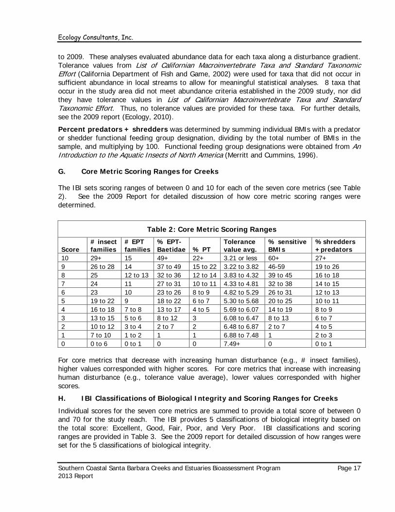
The IBI sets scoring ranges of between 0 and 10 for each of the seven core metrics (see Table 2). See the 2009 Report for detailed discussion of how core metric scoring ranges were determined.

Table 2: Core Metric Scoring Ranges

Score # insect families

# EPT families

% EPT- Baetidae % PT

Tolerance value avg.

% sensitive BMIs

%shredders +predators

10 29+ 15 49+ 22+ 3.21 or less 60+ 27+ 9 26 to 28 14 37 to 49 15 to 22 3.22 to 3.82 46-59 19 to 26 8 25 12 to 13 32 to 36 12 to 14 3.83 to 4.32 39 to 45 16 to 18 7 24 11 27 to 31 10 to 11 4.33 to 4.81 32 to 38 14 to 15 6 23 10 23 to 26 8 to 9 4.82 to 5.29 26 to 31 12 to 13 5 19 to 22 9 18 to 22 6 to 7 5.30 to 5.68 20 to 25 10 to 11 4 16 to 18 7 to 8 13 to 17 4 to 5 5.69 to 6.07 14 to 19 8 to 9 3 13 to 15 5 to 6 8 to 12 3 6.08 to 6.47 8 to 13 6 to 7 2 10 to 12 3 to 4 2 to 7 2 6.48 to 6.87 2 to 7 4 to 5 1 7 to 10 1 to 2 1 1 6.88 to 7.48 1 2 to 3 0 0 to 6 0 to 1 0 0 7.49+ 0 0 to 1

For core metrics that decrease with increasing human disturbance (e.g., # insect families), higher values corresponded with higher scores. For core metrics that increase with increasing human disturbance (e.g., tolerance value average), lower values corresponded with higher scores.

H. IBI Classifications of Biological Integrity and Scoring Ranges for Creeks

Individual scores for the seven core metrics are summed to provide a total score of between 0 and 70 for the study reach. The IBI provides 5 classifications of biological integrity based on the total score: Excellent, Good, Fair, Poor, and Very Poor. IBI classifications and scoring ranges are provided in Table 3. See the 2009 report for detailed discussion of how ranges were set for the 5 classifications of biological integrity.



Table 3 Classifications of Biological Integrity and Scoring Ranges (Creeks)

Category Scoring Range

Excellent 61 to 70

Good 48 to 60

Fair 31 to 47

Poor 9 to 30

Very Poor 0 to 8

I. BMI Community Metrics for Estuaries

17 BMI community metrics were calculated for the study estuaries, including measures of abundance, diversity, disturbance sensitivity, and trophic structure. Many of the metrics calculated have been used effectively as indicators of ecological condition in one or more recent estuarine studies conducted throughout the nation. Table A-4 in the Appendix lists these metrics.

IV. Results and Discussion

A. Physiochemical and Biological Data

Table A-1 in the Appendix provides physiochemical data collected at the creek study reaches this year. Table A-1 also lists BMI taxa and abundances for each creek study reach, as well as BMI density, core metric values, and IBI score. Tolerance values and functional feeding groups are provided for individual BMI taxa. Table A-2 provides a list of the plant species observed at each creek study reach, and the number and percentage of native vs. introduced plant species observed. Table A-3 provides a list of vertebrate species observed at the creek study reaches. For study reaches that have been surveyed multiple times, plant and vertebrate species observations are combined. Table A-4 provides physiochemical and BMI data and metrics for the study estuaries.

B. IBI Scores and Classifications (Creeks)

Table A-5 lists core metric values, IBI scores, and classifications of biological integrity for the study reaches in 2013. Table A-5 also provides the range of IBI scores and classifications of biological integrity for the study reaches in all years of study. The following discusses IBI scores at the individual study reaches for 2013, and compares this year’s scores to previous years. Physical habitat conditions and other factors that have likely affected the creek biota are also discussed.

1. City of Santa Barbara Study Creeks

Sycamore Creek

Drought conditions the past two years caused decreased stream width, depth, and flow in Sycamore Creek this year. For the first time in 11 years of studying SY1, dry conditions were



observed during the spring surveys. The upper half of the study reach was dry, while in the downstream half of the study reach pools were present and riffles were reduced to a narrow slow trickle. Stream flow was very low but continuous at SY3. Stream width and depth were relatively low at both study reaches compared to most years.

Water chemistry measurements at SY1 and SY3 were typical of previous years, with low water temperature (16.1 and 16.2 ºC, respectively), optimal dissolved oxygen (7.3 and 8.0 mg/l., respectively), and specific conductance (2,969 and 2,121 µS, respectively). Riparian canopy cover was 98% at SY1 and 95% at SY3, reflective of the mature riparian overstory trees present at both sites. Habitat assessment score at SY1 was 92, reflecting its HIGH DIST designation, while SY3 scored 127, reflecting its MOD DIST designation. Low stream flow had a downward effect on the habitat assessment scores.

IBI score at SY1 was 24 (Poor), which is similar to the last two years, and the highest score recorded in 11 years of study. IBI score at SY3 was 31 (Fair) this year (2013), which is the highest score recorded in 8 years of study, and the first time SY3 has scored above the Poor range. The primary reason for the relative improvement in IBI scores at SY1 and SY3 was a higher proportion of shredder/predator and sensitive taxa (e.g., Tricoptera).

M ission Creek

Stream width, depth, and flow were relatively low at M3 and M4 due to the drought conditions. Flow in riffles was reduced to a trickle, but flow was continuous in both study reaches. Water chemistry measurements at M3 and M4 were typical of previous years, with low water temperature (15.6 and 15.4 ºC, respectively), good to optimal dissolved oxygen (6.3 and 9.0 mg/l., respectively), and low specific conductance (1,209 and 976 µS, respectively). Riparian canopy cover was 95% at M3 and 93% at M4, reflective of the mature riparian overstory trees present at both sites. Habitat assessment scores were lower than normal at these study reaches (148 at M3 and 165 at M4) due to lower than normal stream flow.

IBI score at M3 was 29 (Poor), which is the third lowest in 13 years of study. M3 typically scores Fair or Good, and has been as high as the Excellent range. This study reach has been known to go dry in the summer/fall months in drought years. This is a probable cause of the lower IBI score this year, as the stream would be in a state of recovery following a dry period. IBI score at M4 was 48 this year, or the bottom of the Good range. M4 typically scores in the Good to Excellent range. There was a higher than normal proportion of Chironomids and non-insect taxa, which has been a typical trend in drought years and can cause a downward trend on IBI score at sites that typically score in the Good to Excellent range.

California newts (Taricha torosa) were observed at M4 this year, but not at M3. Rainbow trout (Oncorhynchus mykiss) were not observed at M3 or M4 this year. These vertebrates are considered indicator species and were regularly observed at both study reaches prior to the Jesusita Fire in May 2009.

Stream flow in M1 and M2 was low, but higher than in the upstream study reaches (M3 and M4). Return flows from urban uses are a significant contributor to overall stream flow at M1 and M2. Water chemistry measurements at M1 and M2 were typical of previous years, with moderate to high water temperature (23.3 and 18.5 ºC, respectively), good to optimal dissolved oxygen (9.0 and 9.5 mg/l., respectively), and moderate specific conductance (1,471 and 1,454 µS, respectively). Riparian canopy cover was 67% at M1, which contributes to higher stream



temperature, and 95% at M2. Habitat assessment score was low at M1 (93) similarly to previous years, and indicative of its HIGH DIST condition. M2 scored slightly better (111), mostly due to the maturing riparian vegetation that has been restored at the site.

IBI score at M1 was 3 (Very Poor) this year. IBI score has been in the Very Poor or lower Poor range at this study reach in all 13 years of study. M2 had an IBI score of 14 (Poor) this year. IBI score has ranged from 5 to 14 at M2 in 10 years of study.

Arroyo Burro

Since the Jesusita Fire burned approximately 70 percent of its upstream watershed in May 2009, there has been notable improvement in habitat conditions at AB3, with less fine sediment, deeper pools, and more exposed hard substrate. The riparian canopy, which was burned out by the fire, is still largely open, and it will likely take several years for it to recover fully. There has, however, been considerable regrowth of the understory plants, and some of the larger canopy trees have survived the fire as evidenced by new growth. Riparian canopy cover improved to 77 percent this year. Water temperatures were cooler last year (14.9ºC) and this year (15.4ºC) compared to 2010. Drought conditions reduced stream flow at AB3 mostly to standing pools at the time of the spring survey. Riffles were mostly dry, with only a faint trickle present in some areas. The lack of flow caused low dissolved oxygen (3.6 mg/l), and specific conductance was higher than normal (2,240 µS).

IBI score at AB3 improved to 33 (Fair) in 2012, its highest score since 2006. This year (2013), IBI score dropped to 12 (Poor), or the second lowest score recorded at AB3 in 13 years of study. There was a higher than normal proportion of Chironomids and non-insect taxa at AB3 this year, which has been a typical trend in drought years. Insect and EPT diversity were also low relative to some years, as was the percentage of EPT taxa. The intermittency of stream flow at this site over the years is now thought to be the primary reason for the large variability in IBI scores (11 to 62) observed over the years. AB3 has been observed to go completely dry in the summer in drought years such as 2012 and 2013. It is not currently known to what degree upstream water diversions are contributing to the intermittency of flow at this study reach.

Downstream study reach AB1 (HIGH DIST) had habitat assessment score (119), water chemistry, and riparian canopy cover (80%) within the ranges from previous years. IBI score was 26 (Poor) this year, the highest score recorded in 11 years of study.

AB5 (HIGH DIST), a habitat restoration site along the lower watershed tributary Mesa Creek, was daylighted in 2007 (i.e., it was formerly an underground storm drain). It has a small watershed area, narrow channel bottom (2 to 3 feet wide), and poorly developed substrate that consists mostly of soft muds and bedrock, with some angular gravel and cobble. Planted in 2007, the riparian vegetation at this site has become very dense, with tree heights of more than 25 feet and riparian canopy cover of 100 percent. Stream temperature was cool (16.3 ºC) as in the last few years, and specific conductance was again very high (4,112 µS). Mineral concentrations are presumed to be high naturally in this creek. IBI score was 10 (Poor), compared to 14 in 2012. IBI score at AB5 has ranged from 3 to 14 in 7 years of study.



2. County of Santa Barbara Study Creeks

Carpinteria Creek

C1 had a habitat assessment score of 94 this year. Habitat assessment score has varied widely (88 to 142) at this site in 12 years of study, primarily due to episodic clearing of the stream channel and riparian corridor for flood control purposes. Very low stream flow depressed the score this year. Riparian canopy cover was 75 percent, stream temperature was low (15.8 ºC), and specific conductance was moderately high (1,568 µS) as in most previous years. Dissolved oxygen was good at 6.2 mg/l this year, and has varied from 5.0 to 14.0 mg/l over the years. IBI score at C1 was 3 (Very Poor), and within the range (0 to 11) from 12 years of study. The consistently low IBI scores for C1 over the years are puzzling. While this site is disturbed, it has good substrate dominated by cobble, gravel, and sand, well-defined riffles and pools, natural banks and a decent riparian corridor with numerous mature canopy trees. Stream flow is perennial except in the driest years. The basic water quality parameters measured have shown signs of disturbance in the form of moderately high conductivity and somewhat variable dissolved oxygen, but not alarmingly so. The watershed has little urban use (3 percent), some agriculture (17 percent), and is mostly undisturbed wilderness (80 percent). Other sites such as R0, RIN0, and SJ2 with similar habitat conditions and watershed characteristics have consistently had much higher IBI scores compared to C1. In fact, several sites with greater watershed and local disturbances such as SY1 and AB1 have consistently higher IBI scores than C1. More detailed analyses of the water chemistry at C1 and determination of upstream water pollutant sources may yield greater understanding of the causes of impairment at this site.

C3, a lightly impacted reference stream reach in Gobernador Creek (Carpinteria Creek tributary), had lower habitat assessment score (144) compared to previous years, primarily due to low stream flow. Water chemistry measurements were favorable as in previous years, with low temperature (13.0 ºC) and specific conductance (795 µS), and optimal dissolved oxygen (9.0 mg/l). Riparian canopy cover was good at 89 percent, a reflection of the mature riparian canopy present at C3. IBI score (46) was on the high end of the Fair range. IBI scores have typically been in the Good to Excellent range at C3.

San Antonio Creek

SA2 had a habitat assessment score of 123. Low stream flow had a downward effect on habitat assessment score. While this stream has little development as a total percentage of its watershed (94% undisturbed open space), heavy sedimentation from orchards proximal to SA2 has been a chronic stressor. This year’s water chemistry readings were similar to previous years, with low temperature (19.2 ºC), moderate specific conductance (1,623 µS) and adequate dissolved oxygen (7.0 mg/l). Riparian canopy cover was excellent at 93 percent due to the mature riparian canopy present at SA2. IBI score (33) was at the low end of Fair. IBI score at SA2 has ranged from 23 to 62 in 9 years of study.

San Jose Creek

SJ2 had a habitat assessment score of 110, which was depressed by the low stream flow conditions. Similar to SA2, heavy sedimentation from upstream orchards has been a chronic problem at SJ2. This year, water temperature was low (17.6 ºC) and dissolved oxygen was



optimal (9.0 mg/l). Specific conductance was higher than normal at SJ2 at 2,320 µS. Riparian canopy cover was 77 percent. IBI score (47) was at the high end of Fair. This was the highest IBI score recorded at SJ2 in 13 years of study.

Arroyo Hondo

Undisturbed study reach AH1 had similar physiochemical parameter values as in previous years of study including high riparian canopy cover (100 percent), optimal dissolved oxygen (8.4 mg/l), and low specific conductance (1,099 µS) and water temperature (14.7 ºC). Habitat assessment score (153) was good, but lower than previous years due to low stream flow. IBI score was 63 (Excellent), which is the highest score of any study reach this year. AH1 typically scores in the Good to Excellent range.

Gaviota Creek

Low gradient GAV1 had a habitat assessment score of 122, which is on the low end of the range from previous years of study. As with the other study reaches, low stream flow had a downward effect on the score. The riparian canopy cover of 58 percent was typical of previous years and reflective of the wide, open, braided channel at this site. Water chemistry was characterized by low stream temperature (14.6 ºC), which is odd for this site, and elevated conductivity (2,029 µS), which has been typical. Dissolved oxygen was optimal (8.1 mg/l). IBI score was 55 (Good), which is the highest score for GAV1 in 10 years of study. The previous high was 50 in 2007.

C. Rainfall and Peak Stream Flow Effects on Creeks

Table A-6 in the Appendix provides yearly rainfall data for the wet season (i.e., September 1 to April 30) from the Santa Barbara County Flood Control District stations in downtown Santa Barbara (elevation 100 feet) and San Marcos Pass (2,300 feet elevation) from 2001-02 to 2012-13. Table A-6 also provides maximum mean daily discharge data from the USGS gauging station in Mission Creek at Rocky Nook Park (near study reach M3) for the same time period.

As shown in the table, local rainfall and peak stream discharges in Mission Creek (as with other local creeks) have varied widely from year to year, as is typical in the region. This past season was very dry, with rainfall totals of 8.68” downtown and 17.50” at San Marcos Pass. These were the 3rd and 4th lowest rainfall totals, respectively at these stations over the past 40 years. The downtown station has a mean annual rainfall of 17.5” in over 130 years of records, with a high of 45” in the 1997-1998 rainy season. The San Marcos Pass station has a mean annual rainfall of 35” in 47 years of records, and a high of 88” in 1982-1983. Maximum mean daily discharge was only 1 cfs in Mission Creek at the Rocky Nook Park gauge this past winter. Mean daily discharge has been as high as 555 cfs in Mission Creek at the Rocky Nook Park gauge over the past 12 years.

Starting in 2002, 9 of the study reaches have been surveyed every year, including a mix of REF (AH1, C3), MOD DIST (AB3, M3, SJ2), and HIGH DIST (AB1, C1, M1, SY1) study reaches. Data is unavailable for 2004, when the County did not conduct bioassessment surveys, and the City study reaches were surveyed using different methodology. In order to analyze the effects of variable rainfall and peak stream flow on local creeks, physiochemical and BMI data for the 9 study reaches was divided into two categories: (1) Wet years and (2) Dry years. Wet years had above average rainfall totals (greater than 17.5” at the downtown Santa Barbara gauge) and



high peak daily stream flow (at least 167 cfs in Mission Creek at Rocky Nook) the previous winter. Dry years had well below average rainfall (12” or less at the downtown Santa Barbara gauge) and low peak daily stream flow (12 cfs or less in Mission Creek at Rocky Nook). In the 11 years studied since 2001-2002 (i.e., excluding 2003-2004), 6 fell into the Wet category, and 5 fell into the Dry category.

As shown in Table A-6, average rainfall at the Downtown and San Marcos Pass gauges was much higher for the Wet years (24.2” and 44.1”, respectively) compared to the Dry years (9.4” and 15.9”, respectively). Likewise, average peak daily stream flow in Mission Creek at Rocky Nook Park was much higher in the Wet years (289 cfs) compared to the Dry years (6 cfs). The wide disparity in rainfall and stream flow conditions between the Wet and Dry categories, coupled with a large data set (11 years, 99 study reaches) and wide range of creek conditions (i.e., REF, MOD DIST, HIGH DIST) studied provides an opportunity to evaluate the impacts of these independent variables (rainfall, stream flow) on the physiochemical and BMI characteristics of local creeks as measured the following spring. Of particular interest is characterizing the impacts of high stream discharges that have occurred during wet winters with high intensity rainfall events. These high stream discharges scour and wash out large quantities of streambed material, as well as invertebrate and vertebrate stream inhabitants. Conversely, deposition of large quantities of alluvial material occurs in lower gradient sections of the streams, covering riffle substrate and filling in pools.

Table A-6 provides mean values for the 9 study reaches for several physiochemical and BMI parameters for each individual year, and by category (i.e., Wet and Dry). Table 4 below provides a summary of selected physiochemical and BMI parameter means for the Wet and Dry year categories.

Table 4 Rainfall/Streamflow Data and Mean Physiochemical/BMI Parameter Values

for 9 Study Reaches, Wet vs. Dry Years, 2002-2013

Cate

gory

Phys

ical

Hab

itat

Scor

e

Stre

am T

empe

ratu

re (

c)

Dis

solv

ed O

xyge

n (m

g/l)

Spec

ific

cond

ucta

nce

(µS

@ 2

5 c)

BMI

Den

sity

(#

/sq.

m)

IBI

Scor

e

# o

f In

sect

Fam

ilies

# o

f EP

T Fa

mili

es

%EP

T -

Baet

idae

% P

T

% S

h+Pr

ed

Tole

ranc

e Va

lue

Aver

age

% S

ensi

tive

BMIs

Bae

tidae

Chi

rono

mid

ae

Sim

ulid

ae

GA

STR

OP

OD

A

OS

TRA

CO

DA

CLA

DO

CE

RA

OLI

GO

CH

AE

TA

Dry 125 16.4 8.3 1470 1006 30 17 7 18 8 11 5.66 22 31 77 11 13 27 7 12

Wet 130 17.2 10.1 1335 874 26 16 7 13 6 8 5.82 14 97 95 23 4 3 2 4



Based on the data available, the following statements can be made with regard to the impacts of variable rainfall and peak stream flows on the 9 study reaches thus far:

• Average physical habitat assessment score has been slightly higher in Wet years (130) compared to Dry years (125). This reflects the fact that some components, namely stream flow and velocity/depth regime, score higher with higher stream flow.

• Water chemistry has been slightly more favorable in Wet years vs. Dry years in the form of higher dissolved oxygen (10.1 mg/l vs. 8.3 mg/l) and lower specific conductance (1,335 µS vs. 1,470 µS). Average stream temperature has been similar in Wet years (17 ºC) and Dry years (16 ºC).

• The data shows evidence of the scouring effects of high stream flows on the BMI community, which appears to be in a state of recovery following Wet years, as evidenced by lower average BMI density (874/m2 compared to 1,006/m2 in Dry years) and lower average IBI score (26 compared to 30 in Dry years). The mild difference in mean IBI score between Wet and Dry years shows that the IBI has some ability to filter out the habitat disruptions caused by heavy scouring flows. The exception to this was 2005, which followed the second wettest year on record, and extreme peak flows (555 cfs peak daily discharge in Mission Creek at Rocky Nook). Mean IBI score in 2005 was only 17, and IBI score range was only 1 to 29. Figure 5 illustrates IBI score by year at the 9 individual study reaches, as well as an average for each year. Another extreme episodic stressor that significantly lowered IBI scores was the string of wildfires that impacted several of the study reaches, most notably M3, M4, and AB3, in 2008 and 2009 (see last year’s report for details).

• Most of the core metrics including % EPT-Baetidae, % PT, % shredders + predators, tolerance value average, and % sensitive BMIs have had better averages in Dry years compared to Wet years. The average number of insect and EPT families has essentially been the same in Wet and Dry years.

• Colonizer taxa Baetidae and Simulidae have been much more prevalent in Wet years, when they have averaged 97 and 23 individuals per site, respectively, compared to Dry years, when they have averaged only 31 and 11 individuals per site, respectively. On the other hand, several non-insect taxa including Gastropoda, Ostracoda, Cladocera, and Oligochaeta have been much more prevalent in Dry years (see Table A-6), indicating that they are scoured out by extreme flows, then become more established with time when low flow conditions persist. Chironomidae have been prevalent and fairly stable in both Wet years (95 individuals per site) and Dry years (77 individuals per site).



D. Estuaries

The following discusses the physiochemical attributes and BMI communities of each individual estuary and their respective watersheds in detail. See Table A-4 for data collected at the study estuaries.

1. Sycamore Creek Estuary

The Sycamore Creek estuary has an upstream watershed of approximately 2,600 acres, including approximately 43 percent wilderness, 55 percent urban development, and 2 percent agriculture (mainly orchards). Upstream of Cabrillo Blvd., the estuary is a channelized extension of Sycamore Creek, and approximately 25-30 feet wide and 3 to 4 feet deep in the center. This section was not surveyed due to access problems. Downstream of Cabrillo Blvd. the estuary stretched along the beach for approximately 60 feet in length and 10 to 20 feet in width at the time of the field survey on October 2. The estuary was closed to the ocean by a natural sand berm of approximately 100 feet wide. Tide conditions were low at the time of the survey (11 AM). The estuary was smaller and shallower compared to last year. Water depth ranged from a few inches along the fringes to 3 feet in the center, and bottom substrate was mostly sand. There was a thin surface layer of fine sediment and organic detritus along most of

0

10

20

30

40

50

60

70

80

2002 2003 2004 2005 2006 2007 2008 2009 2010 2011 2012 2013

IBI S

core

Year

Figure 5: IBI Score by Year for 9 Study Reaches, 2002-2013

C1

C3

SJ2

AH1

SY1

M1

M3

AB1

AB3

AVG



the bottom area, and scattered clumps of submerged algae and seaweed, leaves, twigs, and other organic litter. Fringing vegetation ranged from 0 to 10 feet and width around the estuary, and was composed of approximately 60 percent native and 40 percent non-native cover. There is heavy human traffic in this area from the adjacent roadways, boardwalk, and beach.

Only one sampling location was chosen for this estuary due to its small size. Water surface temperature was 21.2 ºC, salinity was high at 19.1 ppt, dissolved oxygen was 8.1 mg/l, and pH was 8.4. Near the bottom at 3 feet in depth temperature was 20.3 ºC, salinity was 19.2 ppt, and dissolved oxygen was 6.5 mg/l. Overall, the water column was well mixed (i.e., there wasn’t stratification of water chemistry parameters with depth).

This fall, a total of 6 different BMI taxa were observed at the Sycamore Creek estuary, and BMI density was 1,579/m2. Both BMI density and number of taxa were lower compared to last year. Dominant taxa were Corixidae and Ostracoda, and small numbers of Copepoda, Isopoda, Oligochaeta, and Polychaeta were found.

2. Mission Creek Estuary

The Mission Creek estuary has an upstream watershed of approximately 6,900 acres, including approximately 48 percent wilderness, 50 percent urban development, and 2 percent agriculture (mainly orchards). Upstream of Cabrillo Blvd., the estuary is a channelized extension of Mission Creek, and approximately 40 feet wide and 4 to 5 feet deep in the center. This section was not surveyed due to access problems. Downstream of the Cabrillo Blvd. the estuary stretched along the beach for approximately 800 feet in length on October 2, connecting with the Laguna Channel to the east, and was 40 to 50 feet wide. The estuary was closed from the ocean by an approximately 100 feet wide sand berm. Tide conditions were low at the time of the survey. Water depth ranged from a few inches to approximately 5 feet, and bottom substrate was mostly sand. There was a thin surface layer of fine sediment and organic detritus along most of the bottom area, and scattered clumps of submerged algae and seaweed, leaves, twigs, and other organic litter. There are sand dunes along the northern boundary of the estuary and fringing vegetation ranged from 0 to 20 feet in width and was composed of approximately 10 percent native and 90 percent non-native cover. There is heavy human traffic in this area from the adjacent roadways, boardwalk, Stern’s Wharf and the beach.

Sampling locations in the estuary were on the northern bank approximately 100 feet east of the Cabrillo Blvd. bridge, and at the southwestern margin end nearest the ocean. Water chemistry was uniform with location and depth, with temperatures of 20.0 to 21.1 ºC, salinity of 1.0 to 1.2 ppt, dissolved oxygen of 11.6 to 14.7 mg/l, and pH of 8.1 throughout. Sampling depths were approximately 3 feet downstream and 2.5 feet upstream.

A total of 10 different BMI taxa were observed at the Mission Creek estuary this fall, and BMI density was high at 1,765/m2. BMI density and number of taxa were lower compared to last year. Ostracoda were the dominant taxa, and Gastropoda, Corixidae, Chironomidae, Isopoda, and Baetidae were found in significant numbers.

3. Arroyo Burro Estuary

The Arroyo Burro estuary has an upstream watershed of approximately 6,800 acres, including approximately 49 percent wilderness, 4 percent herbaceous open space, 7 percent agriculture (mainly orchards), and 40 percent urban development. The upstream inlet to the estuary is just below the Cliff Drive bridge. The estuary is longer (approximately 1,500 feet) compared to



the Mission Creek and Sycamore Creek estuaries, and 30 to 50 feet wide. The estuary is bordered by natural vegetation and cliffs to the east, and Hendry’s beach and parking area to the west. Sampling locations in the estuary were located approximately 100 feet downstream of the Cliff Dr. bridge (upstream), and at the downstream end near the ocean.

At the upstream site, the estuary was approximately 30 feet wide and 3 to 4 feet deep in the center at the time of the survey on October 3. Bottom substrate was composed mostly of sand, with a thin layer of fine sediments and detritus and scattered algae and leaf litter. Some cobble and gravel was present nearest the upstream end. Thick riparian forest with 90 percent native cover (10 percent non-native) and a minimum width of 25 feet borders this section of the estuary.

At the downstream sampling site, the estuary was approximately 40 feet wide and 4 to 5 feet deep in the center. Bottom substrate was composed of sand with a thin surface layer of fine sediment and organic detritus and scattered submerged algae, seaweed, and other organic litter. The estuary was closed at the time of the survey, which was conducted during low tide conditions. The east side of the lower estuary is bordered by steep hills and cliffs with thick native scrub vegetation, while the west side is abutted by rock rip rap, ornamental shrubs and the Hendry’s beach parking lot. There is moderate to heavy human traffic around the estuary (less upstream) from the adjacent roadways, trails, and Hendry’s beach facility.

Stratification of water temperature, salinity, and dissolved oxygen with depth was observed at both sampling locations, particularly the downstream site. The highly saline downstream site had readings of 25.2 ºC, 11.6 ppt and 12.4 mg/l (pH was 8.0) at the surface, and 22.1 ºC, 27.0 ppt and 7.0 mg/l at 2.5 feet depth. The upstream site was less stratified and less saline, with surface readings of 21.7 ºC, 5.6 ppt, 12.4 mg/l, (pH was 7.8), and readings of 22.1 ºC, 7.5 ppt and 11.4 mg/l at 2 feet depth.

7 different BMI taxa were observed at the Arroyo Burro estuary this fall, and BMI density was 811/m2. Dominant taxa included Corixidae and Ostracoda at the downstream site, while Corixidae were almost completely dominant at the upstream site. Small numbers of Amphipoda, Oligochaeta, Polychaeta, Chironomidae, and Ephydridae were also found.

4. Tecolote Creek Estuary

The Tecolote Creek estuary has an upstream watershed of approximately 3,700 acres, with land cover of approximately 75 percent wilderness, 2 percent herbaceous open space, 19 percent agriculture (mainly orchards), and 4 percent urban development. This estuary has been categorized as MOD DIST based on its watershed land uses. The estuary is long and narrow, extending north to south approximately 500 feet in length, with a width of 40 to 60 feet. The estuary was closed from the ocean by an approximately 30 feet wide sand berm at the time of the October 3 survey, with low tide conditions. Water depth ranged from a few inches to approximately 4 feet, and bottom substrate was mostly sand with some gravel and cobble. There was a thin surface layer of fine sediment and organic detritus along most of the bottom area, and scattered clumps of submerged algae and seaweed, leaves, twigs, and other organic litter. The area surrounding the estuary has been restored and preserved as a natural habitat area, which was presumably a condition of developing the Baccara Resort to the west. Thick riparian scrub and coastal scrub habitat with approximately 90 percent native cover and a width of about 300 feet borders both west and east sides of the estuary. Unpaved trails extend through the habitat area to the beach and a clubhouse that is part of the Baccara Resort. A



footbridge crosses the estuary at its upstream end. Overall, human traffic and noise are light to moderate.

Sampling locations in the estuary were located at the downstream end, and at the upstream end near the footbridge. Water chemistry was well-mixed with respect to depth and longitudinal position. At the downstream end, water temperature was 19.6 ºC at the surface and 19.2 ºC at depth (2 feet). Dissolved oxygen was 10.9 mg/l at the surface to 9.3 mg/l at depth, and salinity was 2.0 ppt throughout the water column. PH was 7.7 at the downstream site. The upstream sampling site was inaccessible by foot due to impenetrable riparian vegetation and steep slopes. Water temperature, (19.1 ºC) dissolved oxygen (10.7 mg/l), and salinity (2.0 ppt) were measured by hanging the YSI probe from the footbridge into the water. These parameters were very similar to those for the downstream site. PH could not be measured with the available equipment.

10 BMI taxa were observed at the estuary, and BMI density was 3,000/m2, which is considerably higher than last year (853/m2). Dominant taxa this year were Chironomidae, Ostracoda, and Baetidae. Corixidae, Isopoda, and Amphipoda were also found in significant numbers.

5. Gaviota Creek Estuary

The Gaviota Creek estuary has an upstream watershed of approximately 12,900 acres, with land cover of approximately 58 percent wilderness, 40 percent herbaceous open space (grazing land), and 2 percent urban development, consisting mostly of roads and park/campground facilities. The estuary is long and narrow, extending north to south approximately 1,500 feet in length, with a width of approximately 30 feet in the upper estuary to approximately 100 feet near the ocean. The estuary was closed from the ocean by an approximately 50 feet wide sand berm at the time of the October 3 survey, with high tide conditions. Water depth ranged from a few inches to approximately 5 feet. In the lower portion of the estuary, bottom substrate was mostly sand with a thin surface layer of fine sediment and organic detritus, and scattered clumps of submerged algae and seaweed, leaves, twigs, and other organic litter. In the upper estuary, substrate was mostly clay and fine sediments, with near vertical clay/soil banks of approximately 6 feet in height.

The estuary is bordered by natural cliffs and coastal/riparian scrub habitat to the east, and the Gaviota State Park parking lot to the west. A coastal scrub/riparian habitat area 30 to 100 feet wide has been preserved/restored as a buffer between the parking lot and the estuary. Native plants compose approximately 80 percent of the vegetative cover surrounding the estuary. Overall, human traffic and noise are light to moderate at the estuary.

Sampling locations in the estuary were located near the downstream and upstream ends. At the downstream end, readings were 14.5 ºC, 7.4 mg/l, and 11.2 ppt at the surface and 14.8 ºC, 6.5 mg/l, and 11.1 ppt at depth (2.5 feet). pH was 8.5. The water chemistry at the upstream site was different, with higher temperature (17.9 ºC at surface and 19.7 ºC at a depth of 2 feet), lower salinity (5.5 ppt at the surface and 6.6 ppt at depth), and low dissolved oxygen (1.7 mg/l throughout the water column). PH was 7.6.

A total of 12 different BMI taxa were observed at the Gaviota Creek estuary, and BMI density was 2,500/m2. Amphipoda were the dominant taxa at the downstream end, and Chironomidae,



Isopoda, and Polychaeta were also found in significant numbers. Dominant taxa at the upstream end were Baetidae and Corixidae, and Chironomidae were also prevalent.

6. Jalama Creek Estuary

The Jalama Creek estuary has an upstream watershed of approximately 16,000 acres, with land cover of approximately 75 percent wilderness, 20 percent grazed annual grasslands, and 5 percent agriculture. There is a small amount of urbanized development in the form of Jalama Road, the County campground (25 acres) and a few scattered ranch houses. Amongst the study estuaries, Jalama has the least disturbed watershed.

The estuary is long and narrow, extending north to south approximately 1,000 feet in length, with a width of 40 to 60 feet. The estuary was open to the ocean at the time of the October 3 survey, with mid-tide conditions. Water depth ranged from a few inches to approximately 5 feet. In the lower portion of the estuary, bottom substrate was mostly sand with a thin surface layer of fine sediment and organic detritus, and scattered clumps of submerged algae and seaweed, leaves, twigs, and other organic litter. In the upper estuary, substrate was mostly sand bottom flanked by soil and bedrock banks of approximately 4 to 15 feet in height. Thick beds of emergent tules and cattails extended from the banks 10 to 15 feet out into the water.

The estuary is bordered by natural hills and riparian scrub habitat to the west. Jalama Beach Park borders the estuary to the east. Sand dunes and vegetation provide a buffer of 30 to 100 feet wide between the estuary and beach park. Native plants compose approximately 80 percent of the vegetative cover surrounding the estuary. Overall, human traffic and noise are light to moderate at the estuary.

Only the lower portion of the estuary was sampled, as the upper portion is inaccessible by foot. Water chemistry readings were 17.4 ºC, 5.6 mg/l, and 0.9 ppt at the surface, and 17.6 ºC, 5.7 mg/l, and 0.9 ppt at depth (2.5 feet). pH was 7.8. Freshwater conditions prevailed throughout the estuary, as was the case last year.

9 BMI taxa were observed at the Jalama Creek estuary, and BMI density was very high at 4,286/m2. Baetidae were the dominant taxa, while Corixidae, Gastropoda, Chironomidae, Ostracoda and Cladocera were common.

Two sensitive aquatic vertebrate species, California red-legged frog and southwestern pond turtle were observed last year at the Jalama estuary, and southwestern pond turtle was observed again this year. Sensitive aquatic vertebrates have not been observed at any of the other study estuaries.

7. Analyses of BMI Metrics Amongst Estuary Groups

Numerous BMI metrics were calculated for each study estuary, including measures of total abundance, diversity, dominance, functional feeding groups, disturbance sensitivity and tolerance, and abundances of individual BMI taxa. Many of the metrics calculated have been useful as ecological indicators in one or more studies of estuaries in various regions of the country. Table A-4 in the appendix provides metric values for each BMI sample and study reach for this year. This information was used to:

1. Further evaluate potential indicator metrics for distinguishing estuary sites along a disturbance gradient, and;



2. Evaluate how variable water chemistry (particularly salinity) affects the BMI community with respect to abundance, diversity, and composition.

Study reaches sampled in 2012 and 2013 (n=12) were grouped by disturbance (i.e., DIST vs. MOD vs. REF). BMI metric means and ranges amongst the 3 disturbance groups were calculated, and are provided in Table A-7. See Figure 6 for means of selected BMI parameters by disturbance group.

Based on the 2012 and 2013 data, BMI metrics that notably increase with disturbance are %COCO (Corixidae+Ostracoda+Cladocera+Oligochaeta) and %tolerant BMIs. BMI metrics that notably decrease with disturbance are %BAIM (Baetidae+Amphipoda+ Isopoda+Mystidacea), %BA (Baetidae+Amphipoda), and %moderately sensitive BMIs. The ratio metrics BA/COCO and mod sensitive/tolerant also appear to have a strong negative relationship with disturbance. All of these metrics show an increasing or decreasing mean value moving from HIGH DIST to MOD DIST to REF groups, and the ranges for the HIGH DIST and REF groups either don’t overlap, or do so only slightly (see Table A-7). These results are consistent with the findings of several other recent estuarine studies showing tolerance metrics as effective indicators of disturbance (Thompson, B. et al., 2011).

BMI metrics that show some increase with disturbance are % predators and % extreme tolerant BMIs. BMI metrics that show some decrease with disturbance are # taxa, % dominant taxa metrics (1, 2, 3, and 4), % collector-gatherers, and % extreme sensitive BMIs. The differences

0

10

20

30

40

50

60

70

80

90

100

Perc

ent

BMI Parameters

Figure 6: Selected BMI Parameter Means by Disturbance Class, 2012 and 2013 Estuaries (n=12)

Hi Dist avg (n=6)

Mod Dist avg (n=2)

REF AVG (n=4)



in means between HIGH DIST and REF are generally smaller for these metrics, and in some cases the mean for MOD DIST is the most extreme (i.e., highest or lowest). There is substantial overlap in the ranges of REF and HIGH DIST groups for these metrics, indicating a looser relationship with disturbance compared to the BMI metrics identified in the paragraph above. Metrics that do not appear to be related to disturbance are BMI density, % insects, and % insects-chironomidae.

Sites sampled in 2012 and 2013 were further divided into 3 salinity classes: low, or “oligohaline” (0.5 to 5 ppt), moderate, or “mesohaline” (5 to 18 ppt), and high, or “polyhaline” (>18 ppt) after the Venice system for estuary classification established by Carriker and Boesch (Thompson et al, 2011). BMI metric means and ranges amongst salinity classes and disturbance groups were calculated and are provided in Table A-7. Figure 7 illustrates the relationship between disturbance and the mean %BAIM and %COCO (i.e., the strongest indicator metrics so far) among the 3 salinity classes with the combined data available from 2012 and 2013.

Interestingly, while salinity certainly shapes the collection of individual BMI taxa present at a given estuary site, it appears thus far to have little influence on the community BMI metrics studied, which appear to be controlled instead by the level of human disturbance. The relationships of BMI community metrics with disturbance observed so far are, with some minor variations, consistent in the low, moderate, and high salinity categories. This tentative conclusion is limited by the fact that no REF sites in the high salinity class have been studied thus far, nor have there been MOD DIST sites in the moderate or high salinity classes.

0 10 20 30 40 50 60 70 80 90

100

Low

Sal

inity

(< 5

ppt)

REF

MOD

DIS

T

DIST

Mod

erat

e Sa

linity

(5-1

8ppt

)

REF

DIST

Hig

h Sa

linity

(>18

ppt)

DIST

Perc

ent

Figure 7: Mean % BAIM and %COCO by Salinity and Disturbance, 2012 and 2013 Study Reaches (n=12)

% BAIM

%COCO



There are notable patterns with respect to common, individual BMI taxa and salinity (see Table A-4). Gastropoda, Mystidacea, and Cladocera have been found only in low salinity. Baetidae and Isopoda have been common in low and moderate salinity, but absent in high salinity. Chironomidae have been common in low and moderate salinity, and have been found in smaller numbers in high salinity. Corixidae, Ostracoda, Oligochaeta, and Amphipoda have been common in all salinities. Polychaeta have been found only in moderate and high salinities.

V. Closing

Over the past 14 years, bioassessment data collected through the Program has provided a wealth of information regarding the physiochemical habitat conditions and biota (particularly the BMI community) present in local streams. The influences of natural physiochemical and climatic variability and human development on local stream communities have been extensively examined. The following general statements can be made based on the research completed thus far:

• Major episodic disturbances including extreme stream flows, drought conditions, and wildfires have been definitively shown to negatively impact stream communities, as evidenced by significantly lower IBI scores and loss or significant reduction of sensitive BMI and vertebrate taxa following such events. Local stream communities have proven to be resilient, typically showing dramatic recovery from extreme episodic disturbances in a year or two. However, some of the more sensitive species (e.g., rainbow trout) have yet to return to streams impacted by recent wildfires, and may require many years to fully recover.

• Negative impacts of human land use on local stream communities (particularly BMIs) have been documented with highly significant statistical test results. Degradation of stream communities (e.g., lower IBI scores and loss of sensitive species), as well as physiochemical habitat conditions, has increased linearly with increased watershed development, and urban development has been shown to have greater impacts on stream communities than has agricultural development.

• Stream habitat restoration sites have shown improved habitat conditions, and in some cases slight improvements in the BMI community over time following restorative actions. Major improvements in stream community condition would likely require larger-scale, watershed-based restorative actions.

12 surveys in 6 study estuaries have been completed over the past two years in the fall. Based on the data available thus far, the BMI metrics that show the greatest differences in means and ranges along a disturbance gradient, and therefore the greatest potential as indicator metrics are: %COCO, %BAIM, %BA, %moderately sensitive BMIs, %tolerant BMIs, BA/COCO and mod sensitive/tolerant BMIs. All of these metrics show an increasing or decreasing mean value moving from HIGH DIST to MOD DIST to REF groups, and the ranges of for the HIGH DIST and REF groups either don’t overlap, or do so only slightly. % predators and % collector-gatherers also show promise, but have more overlap in the ranges between disturbance groups. It is important to point out the limitations of the estuarine data collected thus far, namely: (1) the small sample size (n=12); (2) the small number of estuaries available in the REF category (only 2 in the region identified), and (3) the fact that only one MOD DIST site (Tecolote) has been



sampled thus far. Also, REF conditions have yet to be sampled in the high salinity class. It will be essential to increase the sample size, and fill data gaps in the future to further test, validate (i.e., with statistical significance), and refine potential indicator metrics. Establishing 4 to 6 reliable indicator metrics will be the basis for developing a reliable IBI for local estuaries.

An interesting option to increase sample size would be to treat individual samples from study estuaries as individual sites (i.e., 2 samples have been collected at many of the estuaries). In some cases like Gaviota and Arroyo Burro, water chemistry (particularly salinity) has been different at upstream and downstream sites, and so has BMI community composition. This option would not only increase sample size, but would allow different conditions to be evaluated separately, rather than combined in a single sample. The downside is that the number of BMIs evaluated in each sample would be decreased (i.e., from 300 to 150).

VI. References

Barbour, M.T., J. Gerritsen, B.D. Snyder, and J.B. Stribling. 1999. Rapid Bioassessment Protocols for Use in Creeks and Wadeable Rivers: Periphyton, Benthic Macroinvertebrates and Fish, Second Edition, EPA 841-B-99-002. U.S. Environmental Protection Agency, Office of Water. Washington, D.C.

Bowman, M.L., J. Gerritsen, G.R. Gibson, and B.D. Snyder. 2000. Estuarine and Coastal Waters: Bioassessment and Biocriteria Technical Guidance. U.S. Environmental Protection Agency, Office of Water. Washington, D.C.

Burt, W.H., and R.P. Grossenheider. 1976. A Field Guide to the Mammals, North America North of Mexico. Third Edition. Houghton Mifflin Company. Boston, New York.

California Department of Fish and Game, Aquatic Bioassessment Laboratory. 2002. List of Californian Macroinvertebrate Taxa and Standard Taxonomic Effort. Revised April 30, 2002.

Cooper, S.D., Dudley T.L., and N. Hemphill. 1986. The Biology of Chaparral Streams in Southern California. Proceedings of the Chaparral Ecosystems Research Conference, May 16-17, 1985, Santa Barbara, California. California Water Resources Center, University of California Santa Barbara. Report No. 62. June, 1986.

County of Santa Barbara, Project Clean Water. 2002. Santa Barbara County Coastal Creeks Bioassessment Program, Annual Report, Year 2001.

County of Santa Barbara. 2008. Gap Fire Emergency Watershed Response Plan.

County of Santa Barbara. 2009. Tea Fire Perimeter Map.

County of Santa Barbara. 2009. Jesusita Fire Perimeter Map.

Dale, N. 1986. Flowering Plants, the Santa Monica Mountains, Coastal and Chaparral Regions of Southern California. Published by Capra Press in cooperation with the California Native Plant Society.

ECORP Consulting, Inc. 2005. Results of 2004 Benthic Macroinvertebrate (BMI) Surveys Conducted for the City of Santa Barbara BMI Monitoring Program.



Ecology Consultants, Inc. 2010. Southern Coastal Santa Barbara County Creeks Bioassessment Program, 2009 Report and Updated Index of Biological Integrity.

Hickman, J.C. 1993. The Jepson Manual, Higher Plants of California. University of California Press. Berkeley, CA.

McAuley, M. 1996. Wildflowers of the Santa Monica Mountains. Second Edition. Canyon Publishing Company. Canoga Park, California.

Merritt, R.W. and K.W. Cummins. 1996. An Introduction to the Aquatic Insects of North America, Third Edition. Kendall/Hunt Publishing Company.

Moyle, P.B. 2002. Inland Fishes of California. University of California Press.

Peterson, R.T. 1990. A Field Guide to Western Birds. Third Edition. Houghton Mifflin Company. Boston, New York.

Ranasinghe, J.A., A.M. Barnett, K. Schiff, D.E. Montagne, C. Brantley, C. Beegan, D.B. Cadien, C. Cash, G.B. Deets, D.R. Diener, T.K. Mikel, R.W. Smith, R.G. Velarde, S.D. Watts, and S.B. Weisberg. 2007. Southern California Bight 2003 Regional Monitoring Program: III. Benthic Macrofauna. Southern California Coastal Water Research Project. Costa Mesa, CA.

Stebbins, R.C. 1985. A Field Guide to Western Reptiles and Amphibians. Second Edition. Houghton Mifflin Company. Boston, New York.

Stewart, B.P. and C.R. Nelson. 1994. Nymphs of North American Stonefly Genera (Plecoptera). University of North Texas Press. Denton, Texas.

Thompson, B, Weisberg S, Melwani A, Lowe S, Ranasinghe JA, Cadien DB, Dauer DM, Diaz RJ,

Fields W, Kellogg M et al.. 2011. Low levels of agreement among experts using best professional judgment to assess benthic condition in the San Francisco Estuary and Delta. Ecological Indicators. 12(1):167-173.

United States Geological Survey. Various dates. 7.5 minute quadrangle topographic maps. Weisberg, SB, Thompson B, Ranasinghe JA, Lowe S, Melwani A. 2012. Benthic macrofaunal

assemblages of the San Francisco Estuary and Delta, USA. Environmental Monitoring Assessment

http://www.sfei.org/biblio/author/831










http://www.sfei.org/documents/best-professional-judgment-to-assess-benthic-condition








http://www.sfei.org/documents/benthic-macrofaunal-assemblages-san-francisco-estuary-and-delta-usa

http://www.sfei.org/documents/benthic-macrofaunal-assemblages-san-francisco-estuary-and-delta-usa


APPENDIX

Ecology Consultants, Inc. Table A-1: Creeks Data

Southern Coastal Santa Barbara Creeks and Estuaries Bioassessment Program2013 Report Page A-1

5 2 1 0 2 2 0 0 0 2 3M S S S S S S S S S Scg cg cg cg cg cg p sh p p NA

Stud

y R

each

es

Year

Dis

turb

ance

Gro

up

Ord

er

Elev

atio

n (ft

.)

Gra

dien

t

wat

ersh

ed a

rea

% w

ilder

ness

% u

rban

% a

gric

ultu

re

% h

erba

ceou

s

% u

ndis

turb

ed

Wet

wid

th (m

)

Hab

itat S

core

Stre

am te

mp.

(c)

pH Dis

solv

ed o

xyge

n (m

g/l)

Spec

ific

cond

. (m

icro

S @

25

c)

% ri

paria

n ca

nopy

cov

er

IBI S

core

Cla

ssifi

catio

n of

B I

BM

I den

sity

(#/s

q. m

)

# in

sect

fam

ilies

# EP

T fa

mili

es

% E

PT-B

aetid

ae

%PT

% s

hred

+pre

d

Tol.

Valu

e A

vg.

% s

ensi

tive

BM

Is

Bae

tidae

Cae

nida

e

Emph

emer

ellid

ae

Hep

tage

nida

e

Lept

ohyp

hida

e

Lept

ophl

ebiid

ae

Chl

orop

erlid

ae

Nem

ourid

ae

Perli

dae

Perlo

dida

e

Bra

chyc

entr

idae

C1 2013 MOD DIST 4 15 0.01 9598 80 3 17 0 80 5 94 15.8 7.6 6.2 1568 75 3 Very Poor 173 3 1 0 0 157 1 7.88 2 1 0 0 0 0 0 0 0 0 0 0C3 2013 REF 3 420 0.03 4517 100 0 0 0 100 5 144 13.0 7.9 9.0 795 89 46 Fair 398 22 9 33 13 295 17 5.40 36 15 48 5 0 7 0 0 0 0 0 0SY1 2013 HIGH DIST 3 30 0.01 2482 45 53 2 0 45 2 92 16.1 8.0 7.3 2969 98 24 Poor 660 11 5 5 5 300 9 5.43 4 4 0 0 0 0 0 0 0 0 0 1SY3 2013 MOD DIST 3 170 0.03 1956 52 46 2 0 52 4 127 16.2 7.6 8.0 2121 95 31 Fair 750 15 5 17 17 300 15 6.52 11 7 0 0 0 0 0 0 0 0 0 6M1 2013 HIGH DIST 3 40 0.01 6799 49 49 2 0 49 5 93 23.3 7.7 9.0 1471 67 3 Very Poor 750 5 2 0 0 309 4 7.76 0 8 0 0 0 0 0 0 0 0 0 1M2 2013 HIGH DIST 1 50 0.02 643 24 76 0 0 24 3 111 18.5 8.0 9.5 1454 95 14 Poor 1065 5 1 2 2 297 7 6.05 4 0 0 0 0 0 0 0 0 0 0 0M3 2013 MOD DIST 3 400 0.07 4142 79 18 2 0 79 4 148 15.6 7.6 6.3 1209 95 29 Poor 440 17 9 12 5 290 11 6.07 18 1 6 0 2 0 13 0 2 0 0 1M4 2013 REF 2 1000 0.08 1376 98 2 0 0 98 4 165 15.4 7.9 9.1 976 93 48 Good 750 26 12 28 9 286 12 5.61 33 1 27 4 2 0 25 0 4 0 0 0AB1 2013 HIGH DIST 3 25 0.01 5646 51 38 7 4 53 5 119 19.6 7.9 9.5 1902 80 26 Poor 1384 15 6 15 15 299 8 7.07 4 13 0 0 0 0 0 0 0 0 0 5AB3 2013 MOD DIST 2 300 0.03 2356 90 3 6 0 90 3 116 15.4 7.4 3.6 2240 77 12 Poor 440 11 5 1 0 301 6 7.16 2 6 0 0 0 0 1 0 0 0 0 0AB5 2013 HIGH DIST 1 10 0.02 275 30 70 0 0 30 2 113 16.3 7.4 7.2 4112 100 10 Poor 330 13 2 1 1 227 6 7.07 0 2 0 0 0 0 0 0 0 0 0 0SA2 2013 MOD DIST 3 500 0.05 2556 94 0 2 4 96 3 123 19.2 7.5 7.0 1623 93 33 Fair 213 16 6 26 1 212 12 5.17 31 7 2 0 1 0 50 0 0 0 0 1SJ2 2013 HIGH DIST 3 120 0.01 3836 81 1 16 1 82 2 110 17.6 7.5 9.0 2360 77 47 Fair 166 16 8 32 23 166 25 5.57 37 1 4 0 0 10 0 0 1 0 0 0AH1 2013 REF 2 150 0.04 2583 100 0 0 0 100 3 153 14.7 7.6 8.4 1099 100 63 Excellent 600 32 16 43 21 298 18 4.13 55 11 30 0 4 26 8 1 8 1 0 0GAV1 2013 MOD DIST 3 25 0.01 12791 59 0 0 41 79 3 122 14.6 7.5 8.1 2029 58 55 Good 1065 16 9 50 17 295 27 4.17 55 4 53 0 0 45 3 0 28 0 0 3

New Tolerance ValueS(0-3), M(4-6), T(7-10 Primary FFG



Stud

y R

each

es

Year

C1 2013C3 2013SY1 2013SY3 2013M1 2013M2 2013M3 2013M4 2013AB1 2013AB3 2013AB5 2013SA2 2013SJ2 2013AH1 2013GAV1 2013

New Tole S(0-3), M( Primary F

3 1 5 5 2 4 4 0 5 2 5 2 3 4 5 5 0 5 9 5 2 0 5 8 8 3 4 6 6 6 5 6 7 3 1 8 8 5 5 3 3 5 5 3 0 5 9S S M M S M M S M S M S S M M M S M T M S S M T T S M M M M M M T S S T T M M S S M M S S M Tsc sc cf ph sh om sh sh cf p sc p sh p sh p cg p p p sc sc p NA cg cg p p NA p cg p cf cg NA p p p p NA p p p p p p p

Glo

ssos

tom

atid

ae

Hel

icop

sych

idae

Hyd

rops

ychi

dae

Hyd

ropt

ilida

e

Lepi

dost

omat

idae

Lept

ocer

idae

Lim

noph

ilida

e

Odo

ntoc

erid

ae

Philo

pota

mid

ae

Poly

cent

ropo

dida

e

Psyc

hom

yiid

ae

Rhy

acop

hilid

ae

Seric

osto

mat

idae

Car

abid

ae

Dry

opid

ae

Dyt

isci

dae

Elm

idae

Gyr

inid

ae

Hal

ipid

ae

Hyd

roph

ilida

e

Psph

enid

ae

Ble

phar

icer

idae

Cer

atop

ogon

idae

Chi

rono

mid

ae

Cul

icid

ae

Dix

idae

Dol

icho

podi

dae

Empi

dida

e

Ephy

drid

ae

Mus

cida

e

Psyc

hodi

dae

Scio

myz

idae

Sim

ulid

ae

Stra

tiom

yida

e

Tipu

lidae

Bel

osto

mat

idae

Cor

ixid

ae

Ger

ridae

Nau

corid

ae

Velii

dae

Aes

hnid

ae

Cal

ypte

rygi

dae

Coe

nagr

ioni

dae

Cor

dule

gast

ridae

Gom

phid

ae

Lest

idae

Libe

llulid

ae

0 0 0 0 0 0 0 0 0 0 0 0 0 0 0 0 0 0 0 0 0 0 0 35 0 0 0 0 0 0 0 0 0 0 3 0 0 0 0 0 0 0 0 0 0 0 00 1 1 0 33 0 0 0 0 0 0 3 1 0 0 4 5 0 0 0 0 0 3 135 1 0 0 1 0 0 1 0 18 0 0 1 0 0 0 2 2 0 1 0 0 1 00 0 11 0 0 0 0 0 0 0 1 0 3 0 0 5 2 0 4 0 0 0 0 18 0 0 0 0 0 0 0 0 1 0 0 0 0 0 0 1 0 0 0 0 0 0 00 0 30 0 0 0 0 0 0 0 0 1 13 0 0 0 5 0 2 0 0 0 4 152 0 1 0 0 0 0 0 0 7 1 3 0 0 1 0 0 0 0 14 0 0 3 00 0 0 0 0 0 0 0 0 0 0 0 0 0 0 0 0 0 1 0 0 0 0 240 0 0 0 0 0 0 0 0 19 0 0 0 0 0 0 0 0 0 0 0 0 0 00 0 0 6 0 0 0 0 0 0 0 0 0 0 0 0 0 0 0 0 0 0 0 103 0 0 0 0 0 0 0 0 0 0 12 0 0 0 0 0 0 0 20 0 0 0 02 0 2 0 0 0 0 0 0 0 0 7 0 0 0 1 17 0 0 0 1 0 9 79 0 0 0 0 0 0 3 0 0 0 0 0 0 0 0 0 0 0 1 0 0 2 06 0 2 0 7 0 0 0 0 5 1 1 0 0 0 0 7 0 1 0 1 0 6 142 0 0 0 1 0 0 1 0 4 0 2 0 0 1 0 0 2 0 1 0 0 7 01 0 6 0 0 0 0 0 25 0 0 0 3 0 0 7 0 0 1 0 0 0 2 95 0 0 0 0 0 0 0 0 35 0 1 0 0 0 0 0 2 0 3 0 0 0 00 0 0 0 0 0 0 0 0 0 0 0 1 0 0 8 1 0 0 0 0 0 0 146 0 1 0 0 0 0 1 0 0 0 2 0 0 1 0 0 0 0 0 0 0 4 00 0 0 0 0 0 0 0 2 0 0 0 0 0 0 7 0 0 4 1 0 0 1 94 0 0 0 2 0 0 1 0 9 0 1 0 0 0 0 0 0 0 4 0 0 0 00 0 0 0 0 0 0 0 0 0 0 0 2 0 0 5 0 0 0 0 2 0 1 57 1 5 0 0 0 0 0 0 0 0 1 0 0 0 0 0 0 0 0 0 0 16 02 0 1 0 0 0 0 0 0 1 0 0 34 0 0 0 7 0 0 0 0 0 4 52 0 1 0 0 0 0 1 0 0 0 2 1 0 0 0 0 0 0 1 0 0 0 02 2 11 1 17 0 0 0 5 7 0 7 0 0 0 1 3 0 0 0 15 0 4 81 0 5 0 0 0 0 9 0 1 1 8 0 0 0 0 14 1 0 1 1 0 0 00 0 0 0 14 0 0 0 0 2 0 0 3 0 0 0 0 0 0 0 0 0 5 72 0 1 0 0 0 0 0 0 0 0 0 0 6 0 0 0 0 0 5 0 0 1 0



Stud

y R

each

es

Year

C1 2013C3 2013SY1 2013SY3 2013M1 2013M2 2013M3 2013M4 2013AB1 2013AB3 2013AB5 2013SA2 2013SJ2 2013AH1 2013GAV1 2013

New Tole S(0-3), M( Primary F

0 3 10 3 5 7 7 9 8 5 8 9 10 4S S T S M T T T T M T T T Mp p cg p sc cg cg cg sh cg cg cg pa p

Cor

ydal

idae

Sial

idae

CO

LLEM

BO

LA

AC

AR

I

GA

STR

OPO

DA

OST

RA

CO

DA

CO

PEPO

DA

CLA

DO

CER

A

DEC

APO

DA

AM

PHIP

OD

A

ISO

POD

A

OLI

GO

CH

AET

A

HIR

UD

INEA

TUR

BEL

LAR

IA

Oth

ers-

no to

lera

nce

valu

es

Chr

ysom

elid

ae

Hyd

raen

idae

Not

onec

tidae

Lepi

dopt

era

Hym

enop

tera

Nem

atom

orph

a

Nem

atod

a

Biv

alvi

a (C

lam

)

0 0 0 0 25 4 0 13 0 0 0 75 0 1 0 0 0 0 0 0 0 60 0 0 0 4 0 0 0 0 0 1 0 0 1 0 0 0 0 0 0 0 30 0 0 4 186 22 24 0 0 0 0 1 0 12 0 0 0 0 0 0 0 00 3 0 0 18 11 1 0 0 0 0 12 0 5 0 0 0 0 0 0 0 00 0 0 0 0 0 0 13 0 2 0 13 0 12 0 0 0 0 0 0 0 00 0 0 0 140 2 4 0 1 0 0 9 0 0 0 0 0 1 0 0 0 00 0 0 0 7 106 0 0 0 0 0 16 0 12 0 0 0 0 0 0 0 10 0 0 0 4 20 0 0 0 0 0 0 0 1 0 0 4 0 0 0 0 00 0 0 0 1 1 0 0 0 1 94 1 0 2 0 0 0 1 0 0 0 00 0 0 0 24 84 0 3 0 0 0 14 0 4 0 0 0 0 0 0 0 00 0 0 0 39 12 12 0 0 2 29 5 0 0 0 0 0 0 0 0 0 00 1 0 0 38 18 1 0 0 0 0 3 0 0 0 0 0 1 0 0 0 00 0 0 0 3 29 0 0 0 0 0 11 0 0 0 0 0 0 0 0 0 00 2 0 2 5 0 1 0 0 0 2 0 0 0 1 0 0 0 0 0 0 10 10 0 0 0 19 3 0 0 10 0 2 0 6 0 0 0 0 0 0 0 5

Ecology Consultants, Inc. Table A-2Plant Species Observed at Creek Study Reaches


Family Common Name Scientific Name Study ReachesSY1 SY3 M1 M2 M3 M4 AB1 AB3 AB5 C1 C3 SA2 SJ2 AH1 GAV1

Native TreesAceraceae Big-leaf maple Acer macrophyllum 1 1Aceraceae Box elder Acer negundo 1 1 1Betulaceae White alder Alnus rhombifolia 1 1 1 1 1 1 1 1 1 1Fagaceae Coast live oak Quercus agrifolia 1 1 1 1 1 1 1 1 1 1 1 1 1Jugulandaceae Southern black walnut Juglans californica 1 1 1 1 1 1 1 1Lauraceae California bay Umbellularia californica 1 1 1 1 1 1Platanaceae Sycamore Platanus racemosa 1 1 1 1 1 1 1 1 1 1 1 1 1 1 1Salicaceae Black cottonwood Populus balsamifera trichocarpa 1 1 1 1 1 1 1 1 1 1 1Salicaceae Fremont cottonwood Populus fremontii fremontii 1 1Salicaceae Arroyo willow Salix lasiolepis 1 1 1 1 1 1 1 1 1 1 1 1 1 1 1Salicaceae Red willow Salix laevigata 1 1 1 1 1 1 1 1 1 1 1 1 1 1Native Shrubs, Vines, and HerbsAnacardiaceae Laurel sumac Malosma laurina 1 1 1 1Anacardiaceae Lemonade berry Rhus integrifolia 1 1 1 1 1 1Anacardiaceae Poison oak Toxicodendron diversilobum 1 1 1 1 1 1 1 1 1 1 1 1 1Asteraceae California sagebrush Artemesia californica 1 1 1 1 1 1 1 1 1 1 1Asteraceae Mugwort Artemesia douglasiana 1 1 1 1 1 1 1 1 1 1 1 1 1 1 1Asteraceae Coyote brush Baccharis pilularis 1 1 1 1 1 1 1 1 1 1 1 1 1Asteraceae Plummer's baccharis Baccharis plummerae plummerae 1 1 1Asteraceae Mulefat Baccharis salicifolia 1 1 1 1 1 1 1 1 1 1Asteraceae California bush sunflower Encelia californica 1 1Asteraceae Prickly ox tongue Picris echioides 1 1 1 1 1 1 1 1 1 1 1Asteraceae Goldenrod Solidager californica 1Asteraceae Canyon sunflower Venegasia carpesioides 1 1 1 1 1 1 1 1 1 1 1Asteraceae Cocklebur Xanthium spinosum 1 1 1 1 1 1 1 1Brassicaceae Watercress Rorippa nasturtium-aquaticum 1 1 1 1 1 1 1 1 1 1 1Caprifoliaceae California honeysuckle Lonicera hispidula var. vacillans 1 1 1 1 1Caprifoliaceae Mexican elderberry Sambucus mexicana 1 1 1 1 1 1 1 1 1 1 1 1 1 1 1Caprifoliaceae Creeping snowberry Symphoricarpos mollis 1 1 1 1 1 1Convolvulaceae Morning glory Calystegia macrostegia cyclostegia 1 1 1Cornaceae Dogwood Cornus sp. 1 1 1 1Crassulaceae Live-forever Dudleya sp. 1Cucurbitaceae Wild cucumber Marah macrocarpus 1 1 1Cyperaceae Sedge Carex sp. 1 1 1 1 1Cyperaceae Cyperus Cyperus spp. 1 1 1 1 1 1 1 1 1 1 1 1Cyperaceae Bulrushes Scirpus spp. 1 1 1 1Datiscaceae Durango root Datisca glomerata 1 1 1 1Dennstaedtiaceae Giant chain fern Woodwardia fimbriata 1 1 1 1 1Dryopteridaceae Wood fern Dryopteris arguta 1 1 1 1 1Equisetaceae Horsetail Equisetum spp. 1 1 1 1 1 1 1 1 1 1 1 1 1Fabacae Wild sweet pea Lathyrus vestitus var. vestitus 1 1 1 1 1 1 1 1 1 1 1 1Fabacae Deerweed Lotus scoparius 1 1Fagaceae Scrub oak Quercus berberdifolia 1 1 1 1 1Grossulariaceae Chapparal currant Ribes malvaceum 1Grossulariaceae Fuscia-flowered gooseberry Ribes speciosum 1 1 1 1 1 1 1 1 1Grossulariaceae Gooseberry Ribes sp. 1 1Hydrophyllaceae Yerba santa Eriodictylon crassifoliumHydrophyllaceae Branching phacelia Phacelia ramosissima 1 1Hydrophyllaceae Fiesta flower Pholistoma auritum var. auritum 1Juncaceae Rushes Juncus spp. 1 1 1 1 1 1




Lamiaceae Purple sage Salvia leucophylla 1 1Lamiaceae Black sage Salvia mellifera 1 1 1 1Lamiaceae Crimson pitcher sage Salvia spathacea 1 1Lamiaceae Wood mint, hedge nettle Stachys bullata 1 1 1 1 1Liliaceae Humboldt lily Lilium humboldtii humboldtii 1 1Onagraceae Willow herb Epilobium ciliatum 1 1 1 1 1 1Onagraceae California fuschia Epilobium canum ssp. canumOnagraceae Hooker's evening primrose Oenothera elata ssp. hirsutissmaOrchidaceae Stream orchid Epipactis gigantea 1Oxalidaceae Oxalis Oxalis albicansPapaveraceae California poppy Eschscholzia californica 1Papaveraceae Bush poppy Dendromecon rigidaPoaceae Giant ryegrass Elymus condensatus 1 1 1 1 1 1 1 1 1 1Polygonaceae Ashyleaf buckwheat Eriogonum cinereum 1Polygonaceae California buckwheat Eriogonum fasciculatum 1Polygonaceae Water smartweed Polygonum amphibium var. emersum 1 1 1 1 1 1 1 1Polypodiaceae California polypody Polypodium californicum 1Potamogetonaceae Pondweeds Potamogeton spp. 1 1 1 1 1 1 1 1 1Pteridaceae Venus-hair fern Adiantum capillus-verneris 1 1 1Ranunculaceae Virgin's bower Clematis ligustifolia 1 1 1 1 1 1 1 1 1 1 1Ranunculaceae Meadow rue Thalictrum fendlerli var. polycarpum 1 1 1 1Rhamnaceae Buck brush Ceanothus cuneatus 1 1 1 1 1Rhamnaceae Hairy-leaved ceanothus Ceanothus oliganthusRhamnaceae Big pod ceanothus Ceanothus megacarpusRhamnaceae Greenbark ceanothus Ceanothus spinosus 1 1Rhamnaceae Coffee berry Rhamnus californica 1 1 1 1Rhamnaceae Redberry Rhamnus crocea 1 1Rhamnaceae Hollyleaf redberry Rhamnus ilicifoliaRosaceae Mountain mahogany Cercocarpus betuloides 1 1 1 1Rosaceae Toyon Heteromeles arbutifolia 1 1 1 1 1 1 1 1 1 1Rosaceae Holly-leaf cherry Prunus ilicifolia 1Rosaceae California rose Rosa californica 1 1 1 1Rosaceae California blackberry Rubus ursinus 1 1 1 1 1 1 1 1 1 1 1 1 1 1Salicaceae Narrow-leaved willow Salix exigua 1 1 1Saururaceae Yerba mansa Anemopsis californica 1Scrophulariaceae Annual paintbrush Castilleja minor ssp. spiralis 1Scrophulariaceae Heart-leaved penstemon Keckiella cordifolia 1 1 1 1Scrophulariaceae Bush monkey flower Mimulus aurantiacus 1 1 1 1 1 1Scrophulariaceae Scarlet monkey flower Mimulus cardinalis 1 1 1 1 1 1 1Scrophulariaceae California figwort Scrophularia californica 1 1 1 1 1 1 1 1 1 1 1Solanaceae White nightshade Solanum douglasi 1 1 1 1 1 1 1 1 1 1Solanaceae Purple nightshade Solanum xanti 1 1 1 1Typhaceae Cattails Typha spp. 1 1 1 1 1 1 1 1 1Urticaceae Stinging nettle Urtica dioica 1 1 1 1Verbenaceae Western vervain Verbena lasiostachys 1Vitaceae Wild grape Vitis gidianaNon-Native Trees 1 1Anacardiaceae Peruvian pepper tree Schinus molleMyoporaceae Myoporum Myoporum laetum 1 1Myrtaceae Eucalyptus Eucalyptus spp. 1 1 1 1 1 1Pittosporaceae Pittosporum Pittosporum sp. 1 1 1 1




Tamaricaceae Tamarisk Tamarisk spp.Non-Native Shrubs, Vines, and Herbs 1Apiaceae Poison hemlock Conium maculatum 1 1 1 1 1 1 1 1 1 1Apiaceae Sweet fennel Foeniculum vulgare 1 1 1 1 1 1 1 1 1 1Apocynaceae Periwinkle Vinca major 1 1 1 1 1 1 1 1 1Araliaceae English ivy Hedera helix 1 1 1 1 1 1 1Asteraceae Thoroughwort Ageratina ademorpha 1 1 1 1Asteraceae Italian thistle Cardus pycnocephalus 1 1Asteraceae Brassbuttons Cortula coronopifolia 1Asteraceae Cudweed Gnaphalium luteo-album 1 1 1 1Asteraceae Cape ivy (formerly German ivy) Senecio mikanioides 1 1 1 1 1 1 1Asteraceae Common sow thistle Sonchus oleraceus 1 1 1 1Asteraceae Milk thistle Silybum marianum 1 1 1 1 1Brassicaceae Black mustard Brassica nigra 1 1 1 1 1 1 1 1 1 1 1Brassicaceae Wild radish Raphanus sativus 1 1 1 1 1 1Caprifoliaceae Japanese honeysuckle Lonicera japonica 1Cyperaceae Cyperus Cyperus spp. 1 1 1 1Euphorbiaceae Castor bean Ricinus communis 1 1 1 1 1 1Fabaceae Broom Cytisus sp. 1Fabaceae Bur-clover Medicago polymorpha ssp. hispida 1 1 1 1 1 1 1Fabaceae Sweetclover Melilotus alba 1 1 1 1Geraniaceae White-stem filaree Erodium moschatum 1Lamiaceae Horehound Marubium vulgare 1Lamiaceae Spearmint Mentha spicata var. spicata 1 1 1 1 1 1 1Oxalidaceae Bermuda buttercup Oxalis pes-caprae 1 1 1Plantaginaceae Common plantain Plantago major 1 1 1 1 1 1 1Poaceae Bent grass Agrostis viridis 1 1 1Poaceae Giant reed Arundo donax 1 1 1Poaceae Wild oats Avena fatua 1 1Poaceae Rescue grass Bromus catharticus 1 1 1 1 1Poaceae Ripgut brome Bromus diandrus 1 1 1 1 1Poaceae Pampas grass Cortaderia selloana 1Poaceae Bermuda grass Cynodon dactylon 1 1 1 1 1 1 1 1Poaceae Harding grass Phalaris aquatica 1 1 1 1 1Poaceae Smilo grass Pipatherum milaceum 1 1 1 1 1 1 1 1 1 1Poaceae Rabbitfoot grass, beard grass Polypogon monspeliensis 1 1 1 1 1 1 1 1 1Polygonaceae Curly dock Rumex crispus 1 1 1 1 1 1Primulaceae Scarlet pimpernel Anagallis arvensis 1 1 1 1 1 1 1Rosaceae Himalayan blackberry Rubus discolor 1 1 1 1 1Scrophulariaceae Water speedwell Veronica anagallis-aquatica 1 1 1 1 1 1 1Solanaceae Tree tobacco Nicotiana glauca 1 1 1 1 1 1 1 1Tropaeolaceae Garden nasturtium Tropaeolum majus 1 1 1 1

# native plant species 19 27 20 37 43 37 30 37 34 35 57 34 33 39 39 -native plant species 22 13 23 15 17 1 26 6 9 21 12 12 16 11 21

Total # plant species 41 40 43 52 60 38 56 43 43 56 69 46 49 50 60% native species 46.3 67.5 46.5 71.2 71.7 97.4 53.6 86.0 79.1 62.5 82.6 73.9 67.3 78.0 65.0

Ecology Consultants, Inc. Table A-3Vertebrate Species Observed at Creek Study Reaches


Study ReachesSY1 SY3 M1 M2 M3 M4 AB1 AB3 AB5 C1 C3 SA2 SJ2 AH1 GAV1

CYPRINIDAE Arroyo chub (introduced) Gila orcutti 1 1GASTEROSTEIDAE Three-spine stickle back Gasterosteus acleatus 1 1 1 1POECILIIDAE Mosquito fish (introduced) Gambusia affinis 1 1SALMONIDAE Steelhead/rainbow trout Oncorhynchus mykiss 1 1 1 1 1BUFONIDAE Western toad Bufo boreas 1 1 1HYLIDAE California tree frog Pseudacris cadaverina 1 1 1HYLIDAE Pacific tree frog Pseudacris regilla 1 1 1 1 1 1 1 1 1 1 1 1 1 1 1SALMANDRIDAE California newt Taricha torosa 1 1 1 1 1ANGUIDAE Alligator lizard Elgaria multicarinata 1 1 1COLUBRIDAE Gopher snake Pituophis melanoleucus 1COLUBRIDAE California mountain kingsnake Lampropeltus zonata 1COLUBRIDAE Two-striped garter snake ThamnophIs hammondii 1 1EMYDIDAE Western pond turtle Clemmys marmorata 1 1 1PHRYNOSOMATIDAE Western fence lizard Sceloporus occidentalis 1 1 1 1 1 1 1 1 1PHRYNOSOMATIDAE Side-blotched lizard Uta stansburiana 1 1VIPERIDAE Western rattlesnake Crotalus viridisACCIPITRIDAE Cooper's hawk Accipiter cooperi 1 1 1 1ACCIPITRIDAE Red-shouldered hawk Buteo lineatus 1 1 1 1 1 1 1 1 1 1ACCIPITRIDAE Red-tailed hawk Buteo jamaicensis 1 1 1 1 1 1 1 1AEGITHALIDAE Bushtit Psaltriparus minimus 1 1 1 1 1 1 1 1 1 1 1ALCEDINIDAE Belted kingfisher Ceryle aclyon 1ANATIDAE Mallard Anas platyrhynchos 1 1 1 1 1 1 1 1 1 1ANATIDAE Cinnamon teal Anas cyanopteraANATIDAE American widgeon Anas americanaAPODIDAE Vaux's swift Chaetura vauxi 1ARDEIDAE Snowy egret Egretta thula 1ARDEIDAE Great blue heron Ardea heriodas 1 1ARDEIDAE Green-backed heron Butorides striatus 1BOMBYCILLIDAE Cedar waxwing Bombycilla cedrorum 1CATHARTIDAE Turkey vulture Cathartes aura 1 1 1 1 1CHARADRIIDAE Killdeer Charadrius vociferus 1COLUMBIDAE Mourning dove Zenaida macroura 1 1 1 1 1 1 1 1 1 1 1 1 1COLUMBIDAE Band-tailed pigeon Columba fasciata 1COLUMBIDAE Rock dove (introduced) Columba livia 1 1 1 1CUCULIDAE Greater roadrunner Geococcyx californianus 1CORVIDAE American crow Corvus brachyrhinchos 1 1 1 1 1 1 1 1 1 1 1CORVIDAE Western scrub-jay Aphelocoma californica 1 1 1 1 1 1 1 1 1 1 1 1 1 1 1CORVIDAE Raven Corvus corax 1EMBERIZIDAE Dark-eyed junco Junco hyemalis 1 1 1 1 1 1EMBERIZIDAE Song sparrow Melospiza melodia 1 1 1 1 1 1 1 1 1 1 1 1 1 1 1EMBERIZIDAE White-crowned sparrow Zonotrichia leucophrys 1 1EMBERIZIDAE California towhee Pipilo crissalis 1 1 1 1 1 1 1 1 1 1 1 1 1EMBERIZIDAE Spotted towhee Pipilo maculatus 1 1 1 1 1 1 1 1 1 1 1 1 1 1EMBERIZIDAE Yellow warbler Dendroica petechiaFALCONIDAE American kestrel Falco sparveriusFRINGILLIDAE House finch Carpodactus mexicanus 1 1 1 1 1 1 1 1 1 1 1 1 1 1FRINGILLIDAE American goldfinch Carduelis tristis 1 1 1 1FRINGILLIDAE Lesser goldfinch Carduelis lawrencei 1 1 1 1 1 1 1 1 1 1HIRUNDINIDAE Cilff swallow Petrochelidon pyrrhonota 1 1 1 1 1 1HIRUNDINIDAE Northern rough-winged swallow Stelgidopteryx serripennis 1 1 1 1 1 1 1HIRUNDINIDAE Tree swallow Tachycineta bicolor 1

Family Common Name Scientific Name

Ecology Consultants, Inc. Table A-3Vertebrate Species Observed at Creek Study Reaches


Study ReachesSY1 SY3 M1 M2 M3 M4 AB1 AB3 AB5 C1 C3 SA2 SJ2 AH1 GAV1Family Common Name Scientific Name

HIRUNDINIDAE Violet-green swallow Trachycineta bicolor 1 1ICTERIDAE Blackbird, red-winged Agelaius phoeniceus 1ICTERIDAE Bullock's northern oriole Icterus galbula bullockii 1ICTERIDAE Hooded oriole Icterus cucullatus 1 1LARIDAE Western gull Larus occidentalis 1 1 1 1MIMIDAE Northern mockingbird Mimus polyglottos 1 1 1 1 1 1MIMIDAE California thrasher Toxostoma redivivum 1ODONTOPHORIDAE California quail Callipepla californica 1 1PARIDAE Plain oak titmouse Baeolopus inornatus 1 1 1 1 1 1 1PARULIDAE Common yellowthroat Geothlypis trichas 1 1 1 1 1 1 1 1 1 1 1 1 1PASSERIAE House sparrow (introduced) Passer domesticus 1 1 1PICIDAE Northern flicker Colaptes aurutus 1 1 1 1 1PICIDAE Acorn woodpecker Melanerpes formicivorus 1 1 1 1 1 1 1 1 1 1PICIDAE Downy woodpecker Picoides pubescens 1PICIDAE Hairy woodpecker Picoides villosus 1PODICIPEDIDAE Clark's grebe Aechmophorus clarkii 1PTILOGONATIDAE Phainopepla Phainopepla nitens 1 1 1RALLIDAE American coot Fulica americana 1REGULIDAE Ruby-crowned kinglet Regulus calendula 1STURNIDAE European starling (introduced) Sturnus vulgaris 1THRAUPIDAE Western tanager Piranga ludoviciana 1 1TIMALIIDAE Wrentit Chamaea fasciata 1 1 1 1 1 1 1 1 1 1TROCHILIDAE Anna's hummingbird Calypte anna 1 1 1 1 1 1 1 1 1 1 1 1 1TROCHILIDAE Rufous hummingbird Selasphorus rufus 1 1 1TROGLODYTIDAE Bewick's wren Thryomanes bewickii 1 1 1 1 1TROGLODYTIDAE Canyon wren Catherpes mexicanus 1 1 1TURDIDAE American robin Turdus migratorius 1TURDIDAE Hermit thrush Catharus guttatusTURDIDAE Swainson's thrush Catharus ustulatus 1TYRANNIDAE Pacific-slope flycatcher Empidonax difficilis 1 1 1 1 1 1 1 1 1 1TYRANNIDAE Black phoebe Sayornis nigricans 1 1 1 1 1 1 1 1 1 1 1 1 1 1 1TYRANNIDAE Western kingbird Tyrannus verticalis 1TYRANNIDAE Western wood-pewee Contopus sordidulus 1CANIDAE Coyote Canis latrans 1 1 1 1 1CERVIDAE Mule deer Odocoileus hemionus 1 1 1 1 1 1DIDELPHIDAE Oppossum (introduced) Didelphis virginiana 1FELIDAE Bobcat Lynx rufus 1 1 1 1 1LEPORIDAE Cottontail rabbit Sylvilagus auduboniLEPORIDAE Brush rabbit Sylvilagus bachmanni 1MEPHITIDAE Striped skunk M. mephitis 1 1PROCYONIDAE Racoon Procyon lotor 1 1 1 1 1 1 1 1 1 1 1 1 1SCIRIDAE Merriam's chipmunk Eutamias merriami 1SCIRIDAE California ground squirrel Spermophilus beecheyi 1 1 1SCIRIDAE Western gray squirrel Sciurus griseus 1TALPIDAE Broad-footed mole Scapanus latimanus 1URSIDAE Black bear Ursus americanus 1

20 26 25 24 29 21 30 35 22 30 36 25 32 35 351 3 2 1 3 4 1 2 1 2 5 3 3 5 4

# vertebrate species# native aquatic vertebrate species

Ecology Consultants, Inc. Table A-4: Estuary Study Reach Data


New Tolerance ValueS(0-3), M(4-6), T(7-10) Primary FFG

Estu

ary

Loca

tion

Year

Surv

ey D

ate

Star

t Tim

e

Air

Tem

p (F

)

Tide

con

ditio

ns

Clo

sed/

Ope

n

wat

ersh

ed a

rea

(acr

es)

% w

ilder

ness

% h

erba

ceou

s

% u

rban

% a

gric

ultu

re

Buf

fer v

eget

atio

n av

g. w

idth

(m)

% N

ativ

e B

uffe

r Veg

etat

ion

Wid

th (m

)

leng

th (m

)

appr

ox. s

urfa

ce a

rea

Max

imum

dep

th (m

)

Dom

inan

t sub

stra

te

RPD

dep

th (c

m)

Wat

er te

mp.

(c) t

op

Wat

er te

mp.

(c) b

otto

m

pH to

p

Dis

solv

ed o

xyge

n (m

g/l)

top

Dis

solv

ed o

xyge

n (m

g/l)

botto

m

Con

duct

ivity

(mS)

top

Con

duct

ivity

(mS)

bot

tom

Salin

ity (p

pt) t

op

Salin

ity p

pt b

otto

m

Mea

sure

men

t dep

th (m

)

BM

I sam

ple

area

(m2 )

# B

MIs

pic

ked

# B

MIs

iden

tifie

d

BM

I de

nsity

(#/m

2 )

# ta

xa

% in

sect

s

%in

sect

s - c

hiro

nom

idae

%no

n-in

sect

s

% d

omin

ant t

axa

% 2

dom

inan

t tax

a

% 3

dom

inan

t tax

a

% 4

dom

inan

t tax

a

Arroyo Burro Lower (core) 2013 sand 0.1 25.2 22.1 8.0 12.4 7.0 19.5 39.7 11.6 27.0 0.8 0.01 75 75 7500 6 3 3 93 79 89 93 97Arroyo Burro Lower (epi) 2013 0.18 75 75 417 4 21 21 79 60 81 91 100Arroyo Burro Upper (epi) 2013 sand 0.1 21.7 22.1 7.8 12.4 11.4 9.3 12.3 5.6 7.5 0.7 0.18 150 150 833 5 93 91 7 91 95 97 99

#DIV/0! #### #### ### ### ### ### ###AB TOT 2013 3-Oct 1600 75 low closed 6200 49 4 40 7 >25 70 1.5 0.37 300 300 811 7 53 52 46 51 88 92 95Mission Creek Lower (core) 2013 sand none 20.6 20.0 8.1 14.7 14.0 1.9 2.0 1.0 1.1 0.9 0.02 5 5 250 3 20 0 80 ### ### ### ###Mission Creek Lower (epi) 2013 0.08 145 145 1813 10 37 28 63 ### ### ### ###Mission Creek Upper (core) 2013 clay 0.1 21.1 20.4 8.1 12.6 11.6 2.0 2.2 1.2 1.2 0.8 0.02 3 3 150 2 33 0 67 ### ### ### ###Mission Creek Upper (epi) 2013 0.05 147 147 2940 7 12 5 88 ### ### ### ###M TOT 2013 2-Oct 1400 65 low closed 6900 48 0 50 2 2 10 1.5 1.2 0.17 300 300 1765 10 24 16 76 46 63 73 82Sycamore Creek Lower (core) 2013 sand 0.1 21.2 20.3 8.4 8.1 6.5 28.4 28.0 19.1 19.2 0.9 0.02 3 3 150 2 0 0 100 67 100 100 100Sycamore Creek Lower (epi) 2013 0.17 297 297 1747 5 57 57 43 57 96 98 99

#DIV/0! #### #### ### ### ### ### ####DIV/0! #### #### ### ### ### ### ###

SYC TOT 2013 2-Oct 1600 65 low closed 2600 43 0 55 2 2 60 1.0 0.19 300 300 1579 6 56 56 44 56 95 98 99Tecolote Creek Lower (core) 2013 sand 0.1 19.6 19.2 7.7 10.9 9.3 3.3 3.3 2.0 2.0 0.7 0.02 150 150 7500 3 78 0 22 ### ### ### ###Tecolote Creek Lower (epi) 2013 0.08 150 150 1875 9 61 47 39 ### ### ### ###Tecolote Creek Upper (wq fro 2013 sand 19.1 10.7 3.3 2.0 0.3 #DIV/0! #### #### ### ### ### ### ###

#DIV/0! #### #### ### ### ### ### ###TEC TOT 2013 3-Oct 1400 70 low closed 3700 75 2 4 19 100 95 1.2 0.10 300 300 3000 10 69 23 31 46 66 83 89Gaviota Creek Lower (core) 2013 sand 0.2 14.5 14.8 8.5 7.4 6.5 15.0 15.0 11.2 11.1 0.8 0.02 58 58 2900 3 34 0 66 ### ### ### ###Gaviota Creek Lower (epi) 2013 0.03 92 92 3067 4 15 0 85 ### ### ### ###Gaviota Creek Upper (core) 2013 clay 0.1 17.9 19.7 7.6 1.7 1.7 8.5 11.6 5.5 6.6 0.5 0.02 15 15 750 4 93 20 13 ### ### ### ###Gaviota Creek Upper (epi) 2013 0.05 135 135 2700 6 100 87 0 ### ### ### ###GAV TOT 2013 3-Oct 800 55 high closed 12900 58 40 2 0 >25 80 1.5 0.12 300 300 2500 12 61 40 39 27 48 67 86Jalama Creek Lower (core) 2013 sand 0.1 17.4 17.6 7.8 5.6 5.7 1.6 1.6 0.9 0.9 0.8 0.02 9 9 450 2 0 0 100 ### ### ### ###Jalama Creek Lower (epi) 2013 0.05 291 291 5820 9 71 63 29 ### ### ### ###

#DIV/0! #### #### ### ### ### ### ####DIV/0! #### #### ### ### ### ### ###

JAL TOT 2013 3-Oct 1030 65 mid open >25 80 1.5 0.07 300 300 4286 9 69 61 31 43 61 74 82

Ecology Consultants, Inc. Table A-4: Estuary Study Reach Data


New Tolerance VS(0-3), M(4-6), T(7 Primary FFG

Estu

ary

Arroyo BurroArroyo BurroArroyo Burro

AB TOTMission CreekMission CreekMission CreekMission CreekM TOTSycamore CreekSycamore Creek

SYC TOTTecolote CreekTecolote CreekTecolote Creek

TEC TOTGaviota CreekGaviota CreekGaviota CreekGaviota CreekGAV TOTJalama CreekJalama Creek

JAL TOT

5 5 5 9 8 8 4 6 6 6 3 8 3 NA NA 3 5 5 9 10 3 5 7 7 9 8 5 3? 8 9 3? 10M M M T T T M M M M S T S NA NA S M M T T S M T T T T M S T T S Tcg sh p p cg cg p p NA p cg p NA p p p p p p cg p sc cg cg cg sh cg cg cg cg cg pa

% p

reda

tors

%co

llect

or-g

athe

rers

% s

ensi

tive

BM

Is (3

or l

ess)

% m

oder

atel

y se

nsiti

ve B

MIs

(5 o

r les

s)

% to

lera

nt B

MIs

(7 o

r mor

e)

% e

xtre

mel

y to

lera

nt B

MIs

(9 o

r mor

e)

mod

sen

sitiv

e/to

lera

nt

% B

aetid

, Am

phi,

Isop

oda,

Mys

tid (B

AIM

)

% B

aetid

ae+A

mph

ipod

a (B

A)

% C

orix

, Ost

ra, C

lado

, Olig

o (C

OC

O)

BA

/CO

CO

Bae

tidae

Dry

opid

ae

Dyt

isci

dae

Hal

ipid

ae

Chi

rono

mid

ae

Cul

icid

ae

Dol

icho

podi

dae

Empi

dida

e

Ephy

drid

ae

Mus

cida

e

Stra

tiom

yida

e

Cor

ixid

ae

Velii

dae

Not

onec

tidae

Ger

ridae

Aes

hnid

ae

Coe

nagr

ioni

dae

Lest

idae

Libe

lulii

dae

CO

LLEM

BO

LA

AC

AR

I

GA

STR

OPO

DA

OST

RA

CO

DA

CO

PEPO

DA

CLA

DO

CER

A

DEC

APO

DA

-Hip

pida

e-Em

erita

ana

loga

AM

PHIP

OD

A-G

amm

arid

ea

Mys

tidac

ea (S

hrim

p)

ISO

POD

A

OLI

GO

CH

AET

A

POLY

CH

AET

A

HIR

UD

INEA

1 93 11 11 84 4 0.13 0 0 84 0.00 0 0 0 0 0 0 0 0 1 0 0 1 0 0 0 0 0 0 0 0 0 0 59 0 0 0 0 0 0 3 8 021 79 0 9 91 9 0.10 9 9 91 0.10 0 0 0 0 0 0 0 0 0 0 0 16 0 0 0 0 0 0 0 0 0 0 45 0 0 0 7 0 0 7 0 091 9 0 2 98 1 0.02 2 2 96 0.02 0 0 0 0 3 0 0 0 0 0 0 137 0 0 0 0 0 0 0 0 0 0 6 0 0 0 3 0 0 1 0 0

##### ### ### ##### ### #### #DIV/0! #### #DIV/0! #### #DIV/0! 0 0 0 0 0 0 0 0 0 0 0 0 0 0 0 0 0 0 0 0 0 0 0 0 0 0 0 0 0 0 0 051 47 3 6 93 4 0.06 3 3 92 0.04 0 0 0 0 3 0 0 0 1 0 0 154 0 0 0 0 0 0 0 0 0 0 110 0 0 0 10 0 0 11 8 00 100 0 0 100 0 0.00 60 0 20 0.00 0 0 0 0 1 0 0 0 0 0 0 0 0 0 0 0 0 0 0 0 0 0 1 0 0 0 0 0 3 0 0 021 69 0 20 80 2 0.25 24 8 54 0.15 10 0 2 0 13 0 0 0 0 0 0 28 0 0 0 0 0 0 0 0 0 15 48 1 3 0 2 0 23 0 0 00 33 0 67 33 0 2.00 0 0 0 #DIV/0! 0 0 0 0 1 0 0 0 0 0 0 0 0 0 0 0 0 0 0 0 0 2 0 0 0 0 0 0 0 0 0 01 78 0 27 73 3 0.36 7 5 65 0.07 7 0 0 0 9 0 0 0 0 0 0 1 0 0 0 0 0 0 0 0 0 32 90 0 4 0 0 0 4 0 0 0

10 73 0 23 77 2 0.30 16 6 58 0.11 17 0 2 0 24 0 0 0 0 0 0 29 0 0 0 0 0 0 0 0 0 49 139 1 7 0 2 0 30 0 0 00 100 0 0 100 0 0.00 67 0 33 0.00 0 0 0 0 0 0 0 0 0 0 0 0 0 0 0 0 0 0 0 0 0 0 1 0 0 0 0 0 2 0 0 057 43 1 1 99 0 0.01 0 0 96 0.00 0 0 0 0 0 0 0 0 0 0 0 168 0 0 0 0 0 0 0 0 0 0 116 8 0 0 0 0 1 1 3 0

##### ### ### ##### ### #### #DIV/0! #### #DIV/0! #### #DIV/0! 0 0 0 0 0 0 0 0 0 0 0 0 0 0 0 0 0 0 0 0 0 0 0 0 0 0 0 0 0 0 0 0##### ### ### ##### ### #### #DIV/0! #### #DIV/0! #### #DIV/0! 0 0 0 0 0 0 0 0 0 0 0 0 0 0 0 0 0 0 0 0 0 0 0 0 0 0 0 0 0 0 0 0

56 44 1 1 99 0 0.01 1 0 95 0.00 0 0 0 0 0 0 0 0 0 0 0 168 0 0 0 0 0 0 0 0 0 0 117 8 0 0 0 0 3 1 3 00 100 0 0 100 4 0.00 0 0 22 0.00 0 0 0 0 117 0 0 0 0 0 0 0 0 0 0 0 0 0 0 0 0 0 27 0 0 0 0 0 0 6 0 0

13 87 0 41 59 1 0.69 49 40 34 1.18 50 0 0 0 21 0 0 0 0 0 0 18 0 0 0 0 1 0 1 0 0 0 33 3 0 0 10 0 13 0 0 0##### ### ### ##### ### #### #DIV/0! #### #DIV/0! #### #DIV/0! 0 0 0 0 0 0 0 0 0 0 0 0 0 0 0 0 0 0 0 0 0 0 0 0 0 0 0 0 0 0 0 0##### ### ### ##### ### #### #DIV/0! #### #DIV/0! #### #DIV/0! 0 0 0 0 0 0 0 0 0 0 0 0 0 0 0 0 0 0 0 0 0 0 0 0 0 0 0 0 0 0 0 0

7 93 0 20 80 2 0.26 24 20 28 0.71 50 0 0 0 138 0 0 0 0 0 0 18 0 0 0 0 1 0 1 0 0 0 60 3 0 0 10 0 13 6 0 00 100 31 66 34 0 1.90 34 34 0 #DIV/0! 0 0 0 0 20 0 0 0 0 0 0 0 0 0 0 0 0 0 0 0 0 0 0 0 0 0 20 0 0 0 18 00 100 0 65 35 0 1.88 80 65 4 15.00 0 0 0 0 14 0 0 0 0 0 0 0 0 0 0 0 0 0 0 0 0 0 4 0 0 0 60 0 14 0 0 0

20 87 0 0 107 27 0.00 0 0 20 0.00 0 0 0 0 11 0 0 0 0 0 0 1 0 0 0 0 0 0 2 0 0 0 0 0 0 0 0 0 0 2 0 042 57 1 45 53 0 0.85 44 44 40 1.09 59 0 0 0 18 0 0 0 0 0 0 54 1 2 0 0 1 0 0 0 0 0 0 0 0 0 0 0 0 0 0 020 80 6 53 47 1 1.14 51 46 20 2.28 59 0 0 0 63 0 0 0 0 0 0 55 1 2 0 0 1 0 2 0 0 0 4 0 0 0 80 0 14 2 18 00 44 0 56 44 0 1.25 0 0 44 0.00 0 0 0 0 0 0 0 0 0 0 0 0 0 0 0 0 0 0 0 0 0 5 4 0 0 0 0 0 0 0 0 0

19 67 1 59 41 5 1.43 45 44 31 1.45 129 0 0 0 26 0 0 0 0 0 0 53 0 0 0 0 0 0 0 0 3 39 20 4 16 0 0 0 1 0 0 0##### ### ### ##### ### #### #DIV/0! #### #DIV/0! #### #DIV/0! 0 0 0 0 0 0 0 0 0 0 0 0 0 0 0 0 0 0 0 0 0 0 0 0 0 0 0 0 0 0 0 0##### ### ### ##### ### #### #DIV/0! #### #DIV/0! #### #DIV/0! 0 0 0 0 0 0 0 0 0 0 0 0 0 0 0 0 0 0 0 0 0 0 0 0 0 0 0 0 0 0 0 0

19 67 1 59 41 5 1.42 43 43 31 1.39 129 0 0 0 26 0 0 0 0 0 0 53 0 0 0 0 0 0 0 0 3 44 24 4 16 0 0 0 1 0 0 0

Table A-5Core Metrics, IBI Scores, and Classifications of Biological Integrity for Creeks Study Reaches, 2013


2013Study # I # EPT % EPT- %PT % sh+ Tol val % sens # I # EPT % EPT- %PT % sh+ Tol val % sensReach fams fams Baetidae p avg. BMIs fams fams Baetidae pred avg. BMIsC1 3 1 0 0 1 7.88 2 0 1 0 0 0 0 2 3 Very Poor 13 0 to 15 Very Poor-PoorC3 22 9 33 13 17 5.40 36 5 5 8 8 8 5 7 46 Fair 13 18 to 69 Poor-ExcellentSY1 11 5 5 5 9 5.43 4 2 3 2 4 6 5 2 24 Poor 11 8 to 24 Very Poor-PoorSY3 15 5 17 17 15 6.52 11 3 3 4 9 7 2 3 31 Fair 8 12 to 31 PoorM1 5 2 0 0 4 7.76 0 0 1 0 0 2 0 0 3 Very Poor 13 0 to 11 Very Poor-PoorM2 5 1 2 2 7 6.05 4 0 1 2 2 3 4 2 14 Poor 10 5 to 14 Very Poor-PoorM3 17 9 12 5 11 6.07 18 4 5 3 4 5 4 4 29 Poor 13 18 to 63 Poor-ExcellentM4 26 12 28 9 12 5.61 33 9 8 7 6 6 5 7 48 Good 8 13 to 64 Poor-ExcellentAB1 15 6 15 15 8 7.07 4 3 3 4 9 4 1 2 26 Poor 11 7 to 26 Very Poor-PoorAB3 11 5 1 0 6 7.16 2 2 3 1 0 3 1 2 12 Poor 13 11 to 62 Poor-ExcellentAB5 13 2 1 1 6 7.07 0 3 1 1 1 3 1 0 10 Poor 7 3 to 14 Very Poor-PoorSA2 16 6 26 1 12 5.17 31 4 3 6 1 6 6 7 33 Fair 9 23 to 62 Poor-ExcellentSJ2 16 8 32 23 25 5.57 37 4 4 8 10 9 5 7 47 Fair 13 20 to 47 Poor-FairAH1 32 16 43 21 18 4.13 55 10 10 9 9 8 8 9 63 Excellent 13 25 to 68 Poor-ExcellentGAV1 16 9 50 17 27 4.17 55 4 5 10 9 10 8 9 55 Good 10 4 to 55 Very Poor-Goodavg 15 6 18 9 12 6 19 4 4 4 5 5 4 4 30

Core metric scoring ranges IBI ClassifcationsScore # I fams # EPT fam% EPT- Baetid% PT %sh+pred Tol val avg % sens BMIs Category Scoring Range

10 29+ 15+ 49+ 22+ 27+ 3.21 or less 60+ Excellent 61 to 70

9 26 to 28 14 37 to 49 15 to 22 19 to 26 3.22 to 3.82 46-59 Good 48 to 60

8 25 12 to 13 32 to 36 12 to 14 16 to 18 3.83 to 4.32 39 to 45 Fair 31 to 47

7 24 11 27 to 31 10 to 11 14 to 15 4.33 to 4.81 32 to 38 Poor 9 to 30

6 23 10 23 to 26 8 to 9 12 to 13 4.82 to 5.29 26 to 31 Very Poor 0 to 8

5 19 to 22 9 18 to 22 6 to 7 10 to 11 5.30 to 5.68 20 to 25

4 16 to 18 7 to 8 13 to 17 4 to 5 8 to 9 5.69 to 6.07 14 to 19

3 13 to 15 5 to 6 8 to 12 3 6 to 7 6.08 to 6.47 8 to 13

2 11 to 12 3 to 4 2 to 7 2 4 to 5 6.48 to 6.87 2 to 7

1 7 to 10 1 to 2 1 1 2 to 3 6.88 to 7.48 1

0 0 to 6 0 0 0 0 to 1 7.49+ 0

IBI Score Range

Classification Range

Years Studied

Core Metric Values Core Metric ScoresIBI

ScoreClassification of

Integrity

Ecology Consultants, Inc. Table A-6: Rainfall/ Streamflow Data and Mean Physiochemical/BMI Parameter Values for 9 Study Reaches, Wet vs. Dry Years

Southern Coastal Santa Barbara Creeks Bioassessment Program2013 Report Page A-12

Cat

egor

y

Year

(s)

Rai

nfal

l Dow

ntow

n Sa

nta

Bar

bara

Rai

nfal

l San

Mar

cos

Pass

Peak

dai

ly Q

Mis

sion

Cre

ek (c

fs)

# D

ays

peak

dai

ly Q

> 1

00 c

fs

Phys

ical

Hab

itat S

core

Stre

am te

mp.

(c)

Dis

solv

ed o

xyge

n (m

g/l)

Spec

ific

cond

. (m

icro

S @

25

c)

BM

I den

sity

(#/s

q. m

)

IBI S

core

# in

sect

fam

ilies

# EP

T fa

mili

es

%EP

T - B

aetid

ae

% P

T

% s

h+pr

ed

Tole

ranc

e Va

lue

Avg

.

% s

ens

BM

Is

Bae

tidae

Chi

rono

mid

ae

Sim

ulid

ae

GA

STR

OPO

DA

OST

RA

CO

DA

CLA

DO

CER

A

OLI

GO

CH

AET

A

Dry 2002 8.8 14.3 5 0 123 15 9.4 1492 1895 37 21 9 23 11 14 5.54 28 18 87 3 10 38 13 7Wet 2003 22.8 35.7 184 1 130 16 10.2 1169 1162 29 18 8 14 7 10 5.82 17 80 96 25 3 11 0 10Wet 2005 36.3 70.0 555 14 135 16 10.4 1290 295 17 13 5 4 3 5 5.78 5 153 73 29 0 0 0 0Wet 2006 21.1 35.5 259 2 136 17 11.3 1310 605 33 18 8 19 8 10 5.23 22 116 78 9 1 1 0 5Dry 2007 6.4 10.8 5 0 126 16 7.0 1436 1717 29 18 7 15 6 11 5.91 21 31 68 11 12 52 7 22Wet 2008 17.6 38.1 167 4 128 18 9.1 1522 1057 28 18 8 14 5 8 6.08 16 67 120 13 3 3 11 2Dry 2009 11.4 18.3 12 0 122 17 8.4 1543 406 26 15 6 16 5 9 5.81 21 47 82 26 3 8 0 3Wet 2010 20.3 39.7 177 2 117 20 10.0 1320 1526 25 15 6 12 6 9 6.02 14 63 105 47 14 2 0 3Wet 2011 27.1 45.5 390 5 133 16 9.5 1400 600 27 16 7 12 7 7 5.98 11 104 101 18 0 1 0 4Dry 2012 11.6 18.6 6 0 137 17 9.0 1145 453 31 15 7 19 11 10 4.78 26 51 52 5 14 9 12 16Dry 2013 8.7 17.5 1 0 119 17 7.6 1735 557 28 15 7 16 9 11 6.27 18 7 98 8 28 27 3 15

Dry 5 9.4 15.9 6 0 125 16 8.3 1470 1006 30 17 7 18 8 11 5.66 22 31 77 11 13 27 7 12Wet 6 24.2 44.1 289 5 130 17 10.1 1335 874 26 16 7 13 6 8 5.82 14 97 95 23 4 3 2 4

Ecology Consultants, Inc. Table A-7: Estuary BMI Metric Means and Ranges by Disturbance and Salinity Groupings


Estu

ary

BM

I de

nsity

(#/m

2 )

# ta

xa

% in

sect

s

%in

sect

s - c

hiro

nom

idae

%no

n-in

sect

s

% d

omin

ant t

axa

% 2

dom

inan

t tax

a

% 3

dom

inan

t tax

a

% 4

dom

inan

t tax

a

% p

reda

tors

%co

llect

or-g

athe

rers

% s

ensi

tive

BM

Is (3

or l

ess)

% m

oder

atel

y se

nsiti

ve B

MIs

(5 o

r les

s)

% to

lera

nt B

MIs

(7 o

r mor

e)

% e

xtre

mel

y to

lera

nt B

MIs

(9 o

r mor

e)

mod

sen

sitiv

e/to

lera

nt

% B

aetid

, Am

phi,

Isop

oda,

Mys

tid (B

AIM

)

% B

aetid

ae+A

mph

ipod

a (B

A)

% C

orix

, Ost

ra, C

lado

, Olig

o (C

OC

O)

BA

/CO

CO

Hi Dist avg (n=6) 2824 9 45 37 54 47 78 88 92 34 63 1 9 91 11 0.10 6 4 79 0.05Range 833-50776 to 12 23-65 9 to 56 35-76 30-56 58-95 73-98 82-993 to 5644-93 0-4 1 to 2377-99 0-50 .01-.30 1 to 16 0-6 57-96 .01-.11

Mod Dist avg (n=2) 1926 11 71 27 29 44 67 87 92 16 84 0 13 87 13 0.15 16 13 39 0.32Range 853-300010 to 1169-73 23-31 27-31 42-46 66-67 83-91 89-957 to 2574-93 0-1 6 to 2080-942 to 24.06-0.267 to 245 to 20 28-49 .1-.71

REF AVG (n=4) 2319 12 50 37 51 38 58 74 85 12 84 4 48 52 2 0.94 57 40 22 1.81Range 688-42869 to 14 23-69 7 to 61 31-77 27-47 48-64 67-79 82-872 to 2067-971 to 6 16-66 34-84 0-5 .19-1.91 43-7110 to 6219-31 55-3.19

low salinity (< 5ppt) (n=6)Hi Dist avg (M) 2382 11 23 13 77 48 67 79 87 7 83 0 18 82 26 0.22 12 6 66 0.10Mod Dist avg (T) 1926 11 71 27 29 44 67 87 92 16 84 0 13 87 13 0.16 16 13 39 0.41REF avg (J) 2487 11 46 34 54 45 62 76 83 11 82 3 37 63 3 0.80 53 27 25 0.97

mod salinity (5-18ppt) (n=4)H Dist avg (S, AB) 2774 8 79 64 21 61 77 90 94 62 39 2 7 93 1 0.08 6 4 77 0.06REF avg (G) 2152 13 53 40 47 30 55 73 86 13 87 4 59 41 1 1.52 61 54 20 2.73

high salinity (>18ppt) (n=3)H Dist avg (S, AB) 2482 6 40 39 59 58 90 95 99 39 60 2 4 95 4 0.05 2 1 93 0.02

Documents

2013 REPORT Prepared for: Creeks Division Prepared By scores for the seven core metrics are summed to provide a total score of between 0 and 70 for the study reach