lable at ScienceDirect

Journal of Environmental Management 154 (2015) 13e21

Contents lists avai

Journal of Environmental Management

journal homepage: www.elsevier .com/locate/ jenvman

A real time method of contaminant classification using conventionalwater quality sensors

Shuming Liu*, Han Che, Kate Smith, Tian ChangSchool of Environment, Tsinghua University, Beijing 100084, China

a r t i c l e i n f o

Article history:Received 2 November 2014Received in revised form20 January 2015Accepted 12 February 2015Available online

Keywords:Contaminant classificationConventional sensorEarly warning systemMahalanobis distanceWater quality

* Corresponding author.E-mail address: shumingliu@tsinghua.edu.cn (S. L

http://dx.doi.org/10.1016/j.jenvman.2015.02.0230301-4797/© 2015 Published by Elsevier Ltd.

a b s t r a c t

Early warning systems are often used to detect deliberate and accidental contamination events in a watersource. After contamination detection, it is important to classify the type of contaminant quickly toprovide support for implementation of remediation attempts. Conventional methods commonly rely onlaboratory-based analysis or qualitative geometry analysis, which require long analysis time or suffer lowtrue positive rate. This paper proposes a real time contaminant classification method, which discrimi-nates contaminants based on quantitative analysis. The proposed method utilizes the Mahalanobisdistance of feature vectors to classify the type of contaminant. The performance and robustness of theproposed method were evaluated using data from contaminant injection experiments and through anuncertainty analysis. An advantage of the proposed method is that it can classify the type of contaminantin minutes with no significant compromise on true positive rate. This will facilitate fast remediationresponse to contamination events in a water system.

© 2015 Published by Elsevier Ltd.

1. Introduction

Water systems are vulnerable to contamination accidents andbioterrorism attacks because they are relatively unprotected andaccessible (USEPA, 2003). In 2005, for example, the Songhua Riverwas contaminated by nitrobenzene from a chemical plant explo-sion, which resulted in a 4-day suspension of water supply serviceto Harbin, China (Wang et al., 2012). More recently, in April 2014,crude oil leaked from a Lanzhou Petrochemical pipeline, poisoningthe water source of a local water plant and introducing hazardouslevels of benzene into the city's tap water, which resulted in sus-pension of water supply service in Lanzhou. In this event, it wasdays before the contamination was detected. One approach foravoiding or mitigating the impact of contamination is to establishan Early Warning System (EWS). EWS should provide a fast andaccurate means to distinguish between normal variations andcontamination events and classify the type of contaminant (Storeyet al., 2011). Ideally, it should be inexpensive, easy to maintain andintegrate into network operations, and reliable, with few falsepositives and negatives (Brussen, 2007).

Although there are different types of deployment of EWS, in

iu).

general, an EWS should contain an event detection module, acontaminant classification module and a remediation module. Thecore of an EWS is that it can detect the presence of contaminationand identify the type of contaminant quickly in order to support theimplementation of remediation attempts. The detection of pres-ence of contamination normally employs online water qualitysensors and/or laboratory-based water quality analysis to gatherwater quality data. Generally, there are two types of online waterquality sensors. The first type refers to non-compound specific orconventional water quality sensors, which are normally used fortesting routine water quality parameters, including pH, chlorine,total organic carbon (TOC), oxidation reduction potential (ORP),conductivity, and temperature. The second type is compoundspecific water quality sensors or advanced sensors, which arecapable of confirmative detection at low concentrations for a spe-cific component and are mainly based on emerging detectiontechnologies (Jeon et al., 2008; van der Gaag and Volz, 2008;Hawkins et al., 2005; Henderson et al., 2009; Marshall et al., 2007).

Although compound specific sensors are capable of confirmativedetection for contaminants at low concentration, their applicationin EWS for contamination detection is not popular since the type ofpotential contaminant is not known a priori. Therefore, it is morereasonable to have conventional water quality sensors in thedetection module of the EWS. An example is the Water SecurityInitiative program in the United States, in which pH, turbidity,

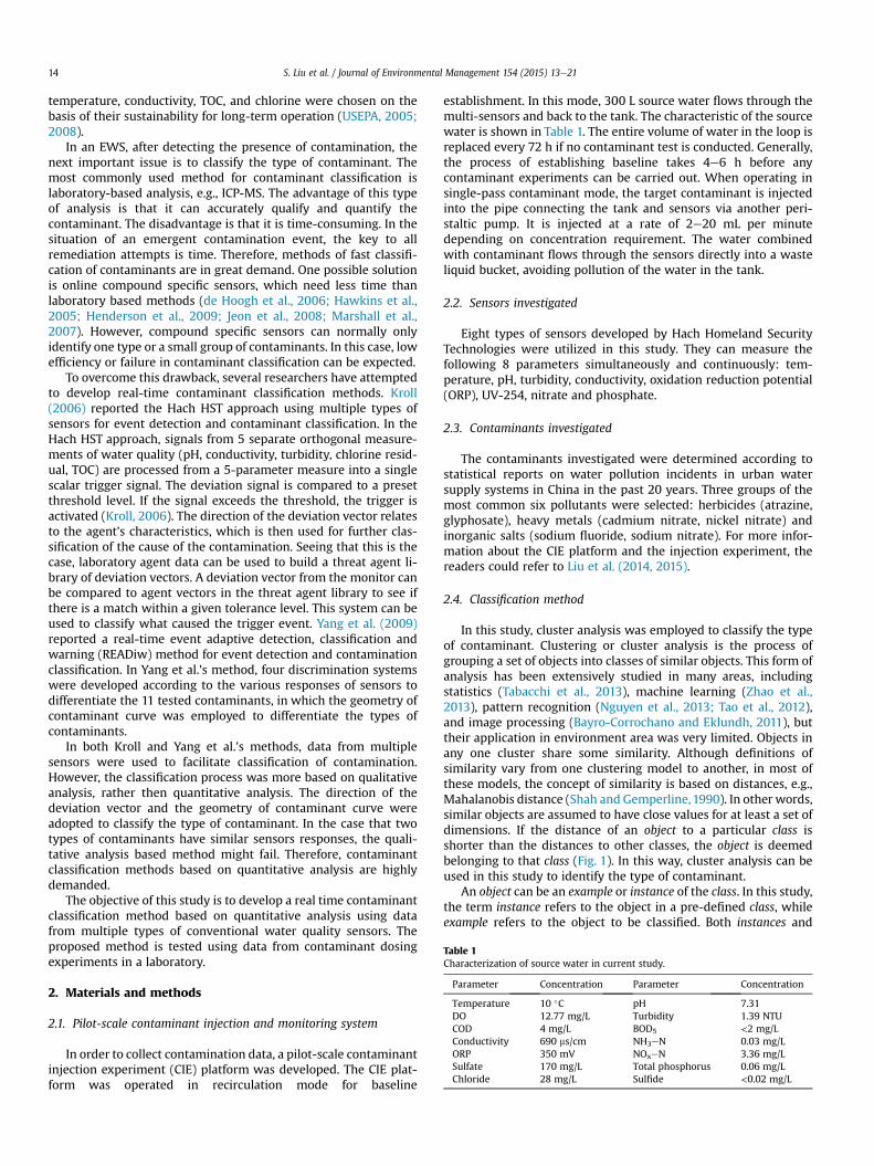
Table 1Characterization of source water in current study.

Parameter Concentration Parameter Concentration

Temperature 10 �C pH 7.31DO 12.77 mg/L Turbidity 1.39 NTUCOD 4 mg/L BOD5 <2 mg/LConductivity 690 ms/cm NH3eN 0.03 mg/LORP 350 mV NOxeN 3.36 mg/LSulfate 170 mg/L Total phosphorus 0.06 mg/LChloride 28 mg/L Sulfide <0.02 mg/L

S. Liu et al. / Journal of Environmental Management 154 (2015) 13e2114

temperature, conductivity, TOC, and chlorine were chosen on thebasis of their sustainability for long-term operation (USEPA, 2005;2008).

In an EWS, after detecting the presence of contamination, thenext important issue is to classify the type of contaminant. Themost commonly used method for contaminant classification islaboratory-based analysis, e.g., ICP-MS. The advantage of this typeof analysis is that it can accurately qualify and quantify thecontaminant. The disadvantage is that it is time-consuming. In thesituation of an emergent contamination event, the key to allremediation attempts is time. Therefore, methods of fast classifi-cation of contaminants are in great demand. One possible solutionis online compound specific sensors, which need less time thanlaboratory based methods (de Hoogh et al., 2006; Hawkins et al.,2005; Henderson et al., 2009; Jeon et al., 2008; Marshall et al.,2007). However, compound specific sensors can normally onlyidentify one type or a small group of contaminants. In this case, lowefficiency or failure in contaminant classification can be expected.

To overcome this drawback, several researchers have attemptedto develop real-time contaminant classification methods. Kroll(2006) reported the Hach HST approach using multiple types ofsensors for event detection and contaminant classification. In theHach HST approach, signals from 5 separate orthogonal measure-ments of water quality (pH, conductivity, turbidity, chlorine resid-ual, TOC) are processed from a 5-parameter measure into a singlescalar trigger signal. The deviation signal is compared to a presetthreshold level. If the signal exceeds the threshold, the trigger isactivated (Kroll, 2006). The direction of the deviation vector relatesto the agent's characteristics, which is then used for further clas-sification of the cause of the contamination. Seeing that this is thecase, laboratory agent data can be used to build a threat agent li-brary of deviation vectors. A deviation vector from the monitor canbe compared to agent vectors in the threat agent library to see ifthere is a match within a given tolerance level. This system can beused to classify what caused the trigger event. Yang et al. (2009)reported a real-time event adaptive detection, classification andwarning (READiw) method for event detection and contaminationclassification. In Yang et al.'s method, four discrimination systemswere developed according to the various responses of sensors todifferentiate the 11 tested contaminants, in which the geometry ofcontaminant curve was employed to differentiate the types ofcontaminants.

In both Kroll and Yang et al.'s methods, data from multiplesensors were used to facilitate classification of contamination.However, the classification process was more based on qualitativeanalysis, rather then quantitative analysis. The direction of thedeviation vector and the geometry of contaminant curve wereadopted to classify the type of contaminant. In the case that twotypes of contaminants have similar sensors responses, the quali-tative analysis based method might fail. Therefore, contaminantclassification methods based on quantitative analysis are highlydemanded.

The objective of this study is to develop a real time contaminantclassification method based on quantitative analysis using datafrom multiple types of conventional water quality sensors. Theproposed method is tested using data from contaminant dosingexperiments in a laboratory.

2. Materials and methods

2.1. Pilot-scale contaminant injection and monitoring system

In order to collect contamination data, a pilot-scale contaminantinjection experiment (CIE) platform was developed. The CIE plat-form was operated in recirculation mode for baseline

establishment. In this mode, 300 L source water flows through themulti-sensors and back to the tank. The characteristic of the sourcewater is shown in Table 1. The entire volume of water in the loop isreplaced every 72 h if no contaminant test is conducted. Generally,the process of establishing baseline takes 4e6 h before anycontaminant experiments can be carried out. When operating insingle-pass contaminant mode, the target contaminant is injectedinto the pipe connecting the tank and sensors via another peri-staltic pump. It is injected at a rate of 2e20 mL per minutedepending on concentration requirement. The water combinedwith contaminant flows through the sensors directly into a wasteliquid bucket, avoiding pollution of the water in the tank.

2.2. Sensors investigated

Eight types of sensors developed by Hach Homeland SecurityTechnologies were utilized in this study. They can measure thefollowing 8 parameters simultaneously and continuously: tem-perature, pH, turbidity, conductivity, oxidation reduction potential(ORP), UV-254, nitrate and phosphate.

2.3. Contaminants investigated

The contaminants investigated were determined according tostatistical reports on water pollution incidents in urban watersupply systems in China in the past 20 years. Three groups of themost common six pollutants were selected: herbicides (atrazine,glyphosate), heavy metals (cadmium nitrate, nickel nitrate) andinorganic salts (sodium fluoride, sodium nitrate). For more infor-mation about the CIE platform and the injection experiment, thereaders could refer to Liu et al. (2014, 2015).

2.4. Classification method

In this study, cluster analysis was employed to classify the typeof contaminant. Clustering or cluster analysis is the process ofgrouping a set of objects into classes of similar objects. This form ofanalysis has been extensively studied in many areas, includingstatistics (Tabacchi et al., 2013), machine learning (Zhao et al.,2013), pattern recognition (Nguyen et al., 2013; Tao et al., 2012),and image processing (Bayro-Corrochano and Eklundh, 2011), buttheir application in environment area was very limited. Objects inany one cluster share some similarity. Although definitions ofsimilarity vary from one clustering model to another, in most ofthese models, the concept of similarity is based on distances, e.g.,Mahalanobis distance (Shah and Gemperline,1990). In other words,similar objects are assumed to have close values for at least a set ofdimensions. If the distance of an object to a particular class isshorter than the distances to other classes, the object is deemedbelonging to that class (Fig. 1). In this way, cluster analysis can beused in this study to identify the type of contaminant.

An object can be an example or instance of the class. In this study,the term instance refers to the object in a pre-defined class, whileexample refers to the object to be classified. Both instances and

Fig. 1. Schematic graphs of class and instance.Fig. 2. Four instances of features of cadmium nitrate and atrazine.

S. Liu et al. / Journal of Environmental Management 154 (2015) 13e21 15

examples are vectors consisting of features. The features areextracted and derived from the sensor responses for contaminants.

2.4.1. Similarity measureA similarity measure is a real-valued function that quantifies the

similarity between two objects. It takes on either zero or smallvalues for similar objects and a large value for very dissimilar ob-jects. The Mahalanobis distance is a unit-less value and a descrip-tive statistic that provides a relative measure of a data point'sdistance from a common point (Mahalanobis, 1936), which canthen be used to identify and gauge similarity of an unknownsample set to a known one. It differs from Euclidean distance in thatit takes into account the correlations of the data set. If p¼ (p1, p2,…, pn) and q¼ (q1, q2, … , qn) are two points in n-space, then theMahalanobis distance from p to q, or from q to p is given by:

DMðp;qÞ ¼ffiffiffiffiffiffiffiffiffiffiffiffiffiffiffiffiffiffiffiffiffiffiffiffiffiffiffiffiffiffiffiffiffiffiffiffiffiffiffiffiffiðp� qÞTS�1ðp� qÞ

q(1)

inwhich DM is the Mahalanobis distance between two points p andq. S is the covariance matrix of q, which is defined as

S ¼ 1n� 1

Xn

i¼1

ðqi � qÞðqi � qÞT (2)

inwhich q is the mean of q. In this study, p and q are n-dimensionalvectors, which contain n feature values. The feature from each timestep forms one vector.

Fig. 2 shows the responses of cadmium nitrate and atrazine attime t1 and t2 for 8 types of sensors. If the sensor reading is taken asthe feature, pt1, pt2, qt1 and qt2 are 8-dimensional vectors. As shownin Fig. 2, the graphs for pt1 and pt2 are more similar, while the graphfor qt1 is closer to the graph for qt2.

2.4.2. Contaminant classificationThe distance from a point p to a class c is given by:

DpcM ðp; cÞ ¼

ffiffiffiffiffiffiffiffiffiffiffiffiffiffiffiffiffiffiffiffiffiffiffiffiffiffiffiffiffiffiffiffiffiffiffiffiffiffiffiffiffiffiffiffiffiffiðp� mcÞTS�1ðp� mcÞ

q(3)

in which, DpcM is the distance from a point to a class and mc is the

mean of all instances in class c.The type of contaminant is identified by comparing the dis-

tances between samples to classes. Assuming there are n types ofcontaminants, c1, c2, … cn, (or n classes), each class contains manyvectors (i.e. instance of class). For any sample p to be identified, ifthere exists

DpcM ðp; ciÞ<Dpc

M

�p; cj

�; j ¼ 1;2; … n; isj (4)

then, it is deemed that p 2 ci.

2.5. Evaluation of classification performance

The performance of the classification method is evaluated usingtrue positive rate (TPR). TPR can be calculated by

TPR ¼ TPTP þ FN

*100% (5)

where TP (true positive) is the correct classification of a contami-nant, FN (false negative) is the incorrect classification of acontaminant as another type of contaminant. A greater TPR meansthe method is more capable of contamination identification.

2.6. Robustness of the proposed method

The proposed method relies on the readings of online waterquality sensors. Inevitably, fluctuations exist in online readings,which might come from equipment noise or ambient environment.An important issue for a contaminant classification method is howrobust it is when dealing with fluctuations in readings. To evaluatethe robustness of the proposed method, artificial uncertaintieswere added to the raw readings. It is assumed that the uncertaintyobeys Gaussian distributions. The uncertainty quantification isachieved through a sampling-based method, Latin hypercubesampling (LHS) technique (Manache and Melching, 2004). In LHS,values of stochastic tested vectors are generated in a random, yetconstrained way. First, taking the values of variables in the originaltested vectors as means (i.e. raw readings of sensors) and a stan-dard deviation equal to 1% of the mean value (i.e. coefficient ofvariation Cv¼ 0.01, for example), the range of each vector variablecan be calculated using a Gaussian distribution equation, which isthen divided intoNs non-overlapping intervals on the basis of equalprobability. After that, a single random value is selected from eachinterval. This process is repeated for all variables in a feature vector.Once that is done, the Ns values obtained for the first vector vari-able are paired in a randommanner with Ns values obtained for thesecond vector variable and so on. Ns feature vectors were generatedfrom the original feature vector. This process is shown in Fig. 3. Byrepeating the same process, feature vectors with uncertainty for alltime steps were obtained. The TPRs for feature vectors with un-certainty can then be obtained.

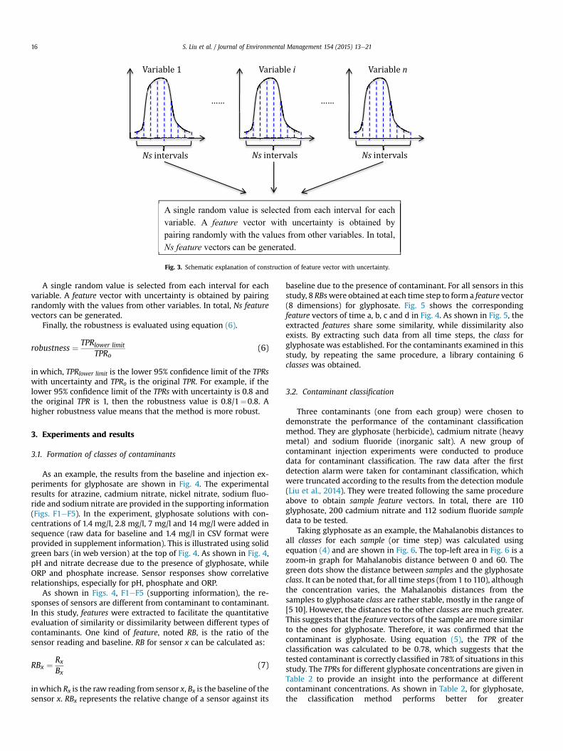
Fig. 3. Schematic explanation of construction of feature vector with uncertainty.

S. Liu et al. / Journal of Environmental Management 154 (2015) 13e2116

A single random value is selected from each interval for eachvariable. A feature vector with uncertainty is obtained by pairingrandomly with the values from other variables. In total, Ns featurevectors can be generated.

Finally, the robustness is evaluated using equation (6).

robustness ¼ TPRlower limit

TPRo(6)

in which, TPRlower limit is the lower 95% confidence limit of the TPRswith uncertainty and TPRo is the original TPR. For example, if thelower 95% confidence limit of the TPRs with uncertainty is 0.8 andthe original TPR is 1, then the robustness value is 0.8/1¼0.8. Ahigher robustness value means that the method is more robust.

3. Experiments and results

3.1. Formation of classes of contaminants

As an example, the results from the baseline and injection ex-periments for glyphosate are shown in Fig. 4. The experimentalresults for atrazine, cadmium nitrate, nickel nitrate, sodium fluo-ride and sodium nitrate are provided in the supporting information(Figs. F1eF5). In the experiment, glyphosate solutions with con-centrations of 1.4 mg/l, 2.8 mg/l, 7 mg/l and 14 mg/l were added insequence (raw data for baseline and 1.4 mg/l in CSV format wereprovided in supplement information). This is illustrated using solidgreen bars (in web version) at the top of Fig. 4. As shown in Fig. 4,pH and nitrate decrease due to the presence of glyphosate, whileORP and phosphate increase. Sensor responses show correlativerelationships, especially for pH, phosphate and ORP.

As shown in Figs. 4, F1eF5 (supporting information), the re-sponses of sensors are different from contaminant to contaminant.In this study, features were extracted to facilitate the quantitativeevaluation of similarity or dissimilarity between different types ofcontaminants. One kind of feature, noted RB, is the ratio of thesensor reading and baseline. RB for sensor x can be calculated as:

RBx ¼ RxBx

(7)

inwhich Rx is the raw reading from sensor x, Bx is the baseline of thesensor x. RBx represents the relative change of a sensor against its

baseline due to the presence of contaminant. For all sensors in thisstudy, 8 RBs were obtained at each time step to form a feature vector(8 dimensions) for glyphosate. Fig. 5 shows the correspondingfeature vectors of time a, b, c and d in Fig. 4. As shown in Fig. 5, theextracted features share some similarity, while dissimilarity alsoexists. By extracting such data from all time steps, the class forglyphosate was established. For the contaminants examined in thisstudy, by repeating the same procedure, a library containing 6classes was obtained.

3.2. Contaminant classification

Three contaminants (one from each group) were chosen todemonstrate the performance of the contaminant classificationmethod. They are glyphosate (herbicide), cadmium nitrate (heavymetal) and sodium fluoride (inorganic salt). A new group ofcontaminant injection experiments were conducted to producedata for contaminant classification. The raw data after the firstdetection alarm were taken for contaminant classification, whichwere truncated according to the results from the detection module(Liu et al., 2014). They were treated following the same procedureabove to obtain sample feature vectors. In total, there are 110glyphosate, 200 cadmium nitrate and 112 sodium fluoride sampledata to be tested.

Taking glyphosate as an example, the Mahalanobis distances toall classes for each sample (or time step) was calculated usingequation (4) and are shown in Fig. 6. The top-left area in Fig. 6 is azoom-in graph for Mahalanobis distance between 0 and 60. Thegreen dots show the distance between samples and the glyphosateclass. It can be noted that, for all time steps (from 1 to 110), althoughthe concentration varies, the Mahalanobis distances from thesamples to glyphosate class are rather stable, mostly in the range of[5 10]. However, the distances to the other classes are much greater.This suggests that the feature vectors of the sample aremore similarto the ones for glyphosate. Therefore, it was confirmed that thecontaminant is glyphosate. Using equation (5), the TPR of theclassification was calculated to be 0.78, which suggests that thetested contaminant is correctly classified in 78% of situations in thisstudy. The TPRs for different glyphosate concentrations are given inTable 2 to provide an insight into the performance at differentcontaminant concentrations. As shown in Table 2, for glyphosate,the classification method performs better for greater

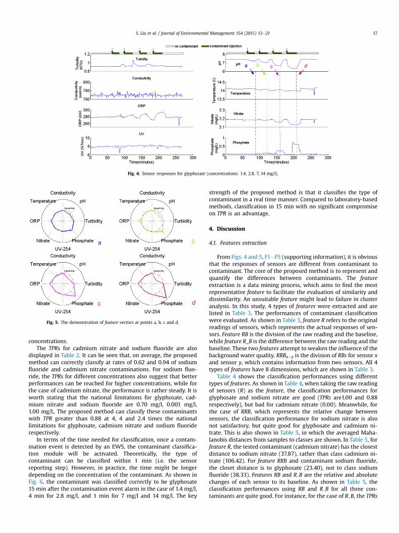
Fig. 4. Sensor responses for glyphosate (concentrations: 1.4, 2.8, 7, 14 mg/l).

Fig. 5. The demonstration of feature vectors at points a, b, c and d.

S. Liu et al. / Journal of Environmental Management 154 (2015) 13e21 17

concentrations.The TPRs for cadmium nitrate and sodium fluoride are also

displayed in Table 2. It can be seen that, on average, the proposedmethod can correctly classify at rates of 0.62 and 0.94 of sodiumfluoride and cadmium nitrate contaminations. For sodium fluo-ride, the TPRs for different concentrations also suggest that betterperformances can be reached for higher concentrations, while forthe case of cadmium nitrate, the performance is rather steady. It isworth stating that the national limitations for glyphosate, cad-mium nitrate and sodium fluoride are 0.70 mg/l, 0.001 mg/l,1.00 mg/L. The proposed method can classify these contaminantswith TPR greater than 0.88 at 4, 4 and 2.4 times the nationallimitations for glyphosate, cadmium nitrate and sodium fluoriderespectively.

In terms of the time needed for classification, once a contam-ination event is detected by an EWS, the contaminant classifica-tion module will be activated. Theoretically, the type ofcontaminant can be classified within 1 min (i.e. the sensorreporting step). However, in practice, the time might be longerdepending on the concentration of the contaminant. As shown inFig. 6, the contaminant was classified correctly to be glyphosate15 min after the contamination event alarm in the case of 1.4 mg/l,4 min for 2.8 mg/l, and 1 min for 7 mg/l and 14 mg/l. The key

strength of the proposed method is that it classifies the type ofcontaminant in a real time manner. Compared to laboratory-basedmethods, classification in 15 min with no significant compromiseon TPR is an advantage.

4. Discussion

4.1. Features extraction

From Figs. 4 and 5, F1eF5 (supporting information), it is obviousthat the responses of sensors are different from contaminant tocontaminant. The core of the proposed method is to represent andquantify the differences between contaminants. The featureextraction is a data mining process, which aims to find the mostrepresentative feature to facilitate the evaluation of similarity anddissimilarity. An unsuitable feature might lead to failure in clusteranalysis. In this study, 4 types of features were extracted and arelisted in Table 3. The performances of contaminant classificationwere evaluated. As shown in Table 3, feature R refers to the originalreadings of sensors, which represents the actual responses of sen-sors. Feature RB is the division of the raw reading and the baseline,while feature R_B is the difference between the raw reading and thebaseline. These two features attempt to weaken the influence of thebackground water quality. RRBx�y is the division of RBs for sensor xand sensor y, which contains information from two sensors. All 4types of features have 8 dimensions, which are shown in Table 3.

Table 4 shows the classification performances using differenttypes of features. As shown in Table 4, when taking the raw readingof sensors (R) as the feature, the classification performances forglyphosate and sodium nitrate are good (TPRs are1.00 and 0.88respectively), but bad for cadmium nitrate (0.00). Meanwhile, forthe case of RRB, which represents the relative change betweensensors, the classification performance for sodium nitrate is alsonot satisfactory, but quite good for glyphosate and cadmium ni-trate. This is also shown in Table 5, in which the averaged Maha-lanobis distances from samples to classes are shown. In Table 5, forfeature R, the tested contaminant (cadmium nitrate) has the closestdistance to sodium nitrate (37.87), rather than class cadmium ni-trate (106.42). For feature RRB and contaminant sodium fluoride,the closet distance is to glyphosate (23.40), not to class sodiumfluoride (38.33). Features RB and R B are the relative and absolutechanges of each sensor to its baseline. As shown in Table 5, theclassification performances using RB and R B for all three con-taminants are quite good. For instance, for the case of R B, the TPRs

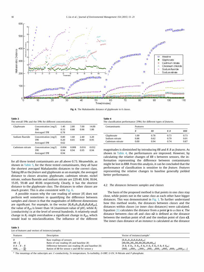
Fig. 6. The Mahalanobis distance of glyphosate to 6 classes.

Table 2The overall TPRs and the TPRs for different concentrations.

Glyphosate Concentration (mg/l) 1.40 2.80 7.00 14.00TPR 0.33 0.88 0.96 1.00Averaged TPR 0.78

Sodium fluoride Concentration (mg/l) 0.80 1.60 2.40 3.20TPR 0.20 0.65 0.90 0.95Averaged TPR 0.62

Cadmium nitrate Concentration (mg/l) 0.004 0.008 0.016 0.032TPR 0.94 0.94 0.95 0.94Averaged TPR 0.94

Table 4The classification performance (TPRs) for different types of features.

Contaminants Features

R RB R B RRB

Glyphosate 1.00 0.78 0.73 0.73Sodium nitrate 0.88 0.62 0.79 0.01Cadmium nitrate 0.00 0.94 0.74 0.87

S. Liu et al. / Journal of Environmental Management 154 (2015) 13e2118

for all three tested contaminants are all above 0.73. Meanwhile, asshown in Table 5, for the three tested contaminants, they all havethe shortest averaged Mahalanobis distances to the correct class.Taking RB as the feature and glyphosate as an example, the averageddistance to classes atrazine, glyphosate, cadmium nitrate, nickelnitrate, sodium fluoride and sodium nitrate are 229.40, 8.04, 18.64,15.05, 59.48 and 40.06 respectively. Clearly, it has the shortestdistance to the glyphosate class. The distances to other classes aremuch greater. This is also consistent with Fig. 6.

A possible reason why the raw reading of sensor (R) does notperform well sometimes in quantifying the difference betweensamples and classes is that the magnitudes of different dimensionsare significant. For example, in the vector [RCRTeRTuRORURNRPRpH],the value of RpH is lower than 14 (maximum value of pH), while RC(conductivity) is at the level of several hundreds. A relatively smallchange in RC might overshadow a significant change in RpH, whichwould lead to misclassification. The influence of the different

Table 3List of features and vectors of instances/samples.

Features Description

R Raw readings of sensorsRB ¼ R

B Ratio of raw reading (R) and baseline (B)R B ¼ R� B Difference between raw reading (R) and baseline (B)RRBx�y ¼ RBx

RByRation of RB for sensor x and RB for sensor y

a The meanings of the subscripts are: C-conductivity, Te-temperature, Tu-turbidity, O-

magnitudes is diminished by introducing RB and R B as features. Asshown in Table 4, the performances are improved. However, bycalculating the relative changes of RB s between sensors, the in-formation representing the difference between contaminantsmight be lost in RRB. From this analysis, it can be concluded that theperformance of classification is sensitive to the feature. Featuresrepresenting the relative changes to baseline generally yieldedbetter performance.

4.2. The distances between samples and classes

The basis of the proposed method is that points in one class stayclose, while points not in the same class as each other have biggerdistances. This was demonstrated in Fig. 1. To further understandhow this method works, the distances between classes and thedistances within classes (or inner class distances) were calculated.Equation (3) calculates the distance from a point p to a class c. Thedistance between class c1 and class c2 is defined as the distancebetween the median point of c1 and the median point of class c2.The inner class distance of an instance is calculated as the distance

Vector of instance/samplea

[RCRTeRTuRORURNRPRpH][RBCRBTeRBTuRBORBURBNRBPRBpH]½R BC R BTe R BTu R BO R BU R BN R BP R BpH �[RRBC�TeRRBTe�TuRRBTu�oRRBO�URRBU�NRRBN�PRRBP�pHRRBpH�C]

ORP, U-UV, N-Nitrate and P-phosphate.

Table 5Averaged Mahalanobis distances from samples to classes.

Tested sample Feature Averaged Mahalanobis distances from samples to classes

Atrazine Glyphosate Cadmium nitrate Nickel nitrate Sodium fluoride Sodium nitrate

Glyphosate R 299.37 19.11 58.62 85.15 309.36 105.55RB 229.40 8.04 18.64 15.05 59.48 40.06R B 213.50 7.70 15.12 13.54 59.79 38.90RRB 75.29 7.73 24.84 17.50 54.61 51.26

Sodium fluoride R 533.46 265.68 249.63 354.56 74.99 115.29RB 41.14 27.68 32.52 32.01 25.60 34.50R B 123.35 51.00 90.64 51.63 37.97 52.21RRB 34.29 23.40 26.34 24.53 38.33 32.36

Cadmium nitrate R 426.85 359.29 106.42 545.87 132.10 37.87RB 211.83 161.00 20.48 277.45 206.79 28.34R B 190.41 199.22 14.28 326.30 184.60 16.36RRB 123.57 64.34 21.52 101.18 110.69 47.53

The bold numbers denote the shortest distance from the tested sample to classes for each feature.The bold numbers with underline indicate the tested sample and the class with shortest distance are not identical.

S. Liu et al. / Journal of Environmental Management 154 (2015) 13e21 19

between the instance to the median point of the class.Table 6 shows the Mahalanobis distance between classes for the

case of feature RB. As shown in Table 6, the Mahalanobis distancesbetween classes differ significantly. For example, the Mahalanobisdistance between sodium nitrate and nickel nitrate is 161.26, whileit is 194,817.77 between cadmium nitrate and nickel nitrate. Thestandard deviation of these distances is 57,198.86, which meansthat these classes are well scattered. This also suggests that featureRB can represent the differences between these feature vectors ofdifferent classes and differentiate them quantitatively.

Fig. 7 shows the inner distances of all instances in the 6 classesunder discussion. As shown in Fig. 7, the inner distances of the 6classes are all below 50 (the majority are smaller than 10).Compared to the distances between classes (Table 6), it is clear thatthe inner distances of classes are much smaller. This justifies theassumption that points in a class share some similarity and stayclose. This also implies that samples can be grouped into pre-defined classes by using the proposed method.

4.3. Robustness

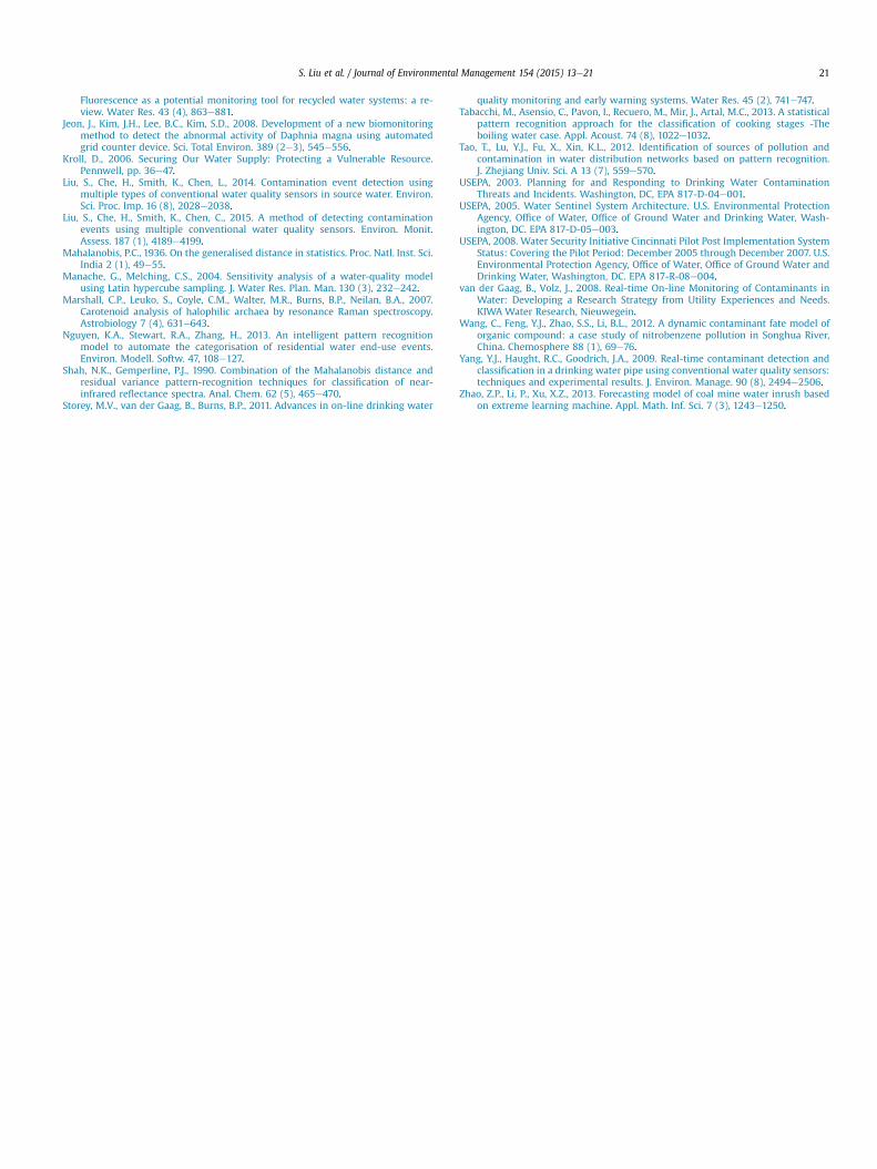
The level of uncertainty is given by the value of Cv. In this study,two values of Cv (0.01 and 0.02) were used. The value of Ns isdetermined according to the literature. For a given Cv, by settingNs¼ 2000, 220,000 feature vectors with uncertainty were finallygenerated for glyphosate. These feature vectors were divided into2000 groups. Each contains 110 feature vectors. By feeding the 2000groups of feature vectors into the proposed contaminant classifi-cation method, the TPRs for every group were obtained. The his-tograms of these TPRs are displayed in Fig. 8, which shows that theproposed method has good robustness for both levels of uncer-tainty (Cv¼ 0.01 and Cv¼ 0.02). In the four tested features, theproposed method has the smallest robustness when the divisionbetween raw reading and baseline (RB) is taken as the feature (0.62,

Table 6Mahalanobis distance between classes (feature RB).

Classes Atrazine Glyphosate Cadmium nitrAtrazine 0.00 412.30 840.02Glyphosate 412.30 0.00 204.46Cadmium nitrate 840.02 204.46 0.00Nickel nitrate 1302.49 449.41 194,817.77Sodium fluoride 1544.21 5462.69 115,602.44Sodium nitrate 246.05 1310.31 194.16

Standard deviation 57,198.86

Cv¼ 0.02). All the others yield high robustness values. In particular,for the case where the difference between raw readings andbaseline (R_B) is used as the feature, the robustness values are 0.99for Cv¼ 0.01 and Cv¼ 0.02. This suggests that the performance ofthe proposed contaminant classification method is steady andreliable and can cope well with the uncertainty from the onlinesensors. It is concluded that, by choosing R_B as the feature, theproposed method has good performance (TPR> 0.73, Table 4) androbustness (0.99, Cv¼ 0.02). It should be noted that the uncertaintyexamined in this study is assumed to be from equipment noise orambient environment. A change of sensor reading due to suddensensor failure or presence of contaminant is not treated as noise,but instead as an event, which normally means a 1e20% change ofsensor reading. Therefore, it is deemed that the uncertainty levelsadopted in this study are significant enough.

4.4. Future works

In the current study, for the purpose of demonstration, a librarycontaining 6 types of contaminants (heavy metals, pesticide/her-bicide and inorganic salts) was established. However, it is envisagedthat more contaminants should be tested in the future to form abigger library for better classification performance. Meanwhile, aprecondition of the discussion in this study that the type ofcontaminant to be tested is included in the predefined library.However, in a real situation, the type of contaminant is not known apriori. Therefore, the performance of the proposed method in thecase that the type of the contaminant to be tested is not included inthe library should be further investigated.

5. Conclusion

By using data from online water quality sensors, this studyproposed a real time contaminant classification method. From the

ate Nickel nitrate Sodium fluoride Sodium nitrate1302.49 1544.21 246.05449.41 5462.69 1310.31194,817.77 115,602.44 194.160.00 1328.31 161.261328.31 0.00 640.15161.26 640.15 0.00

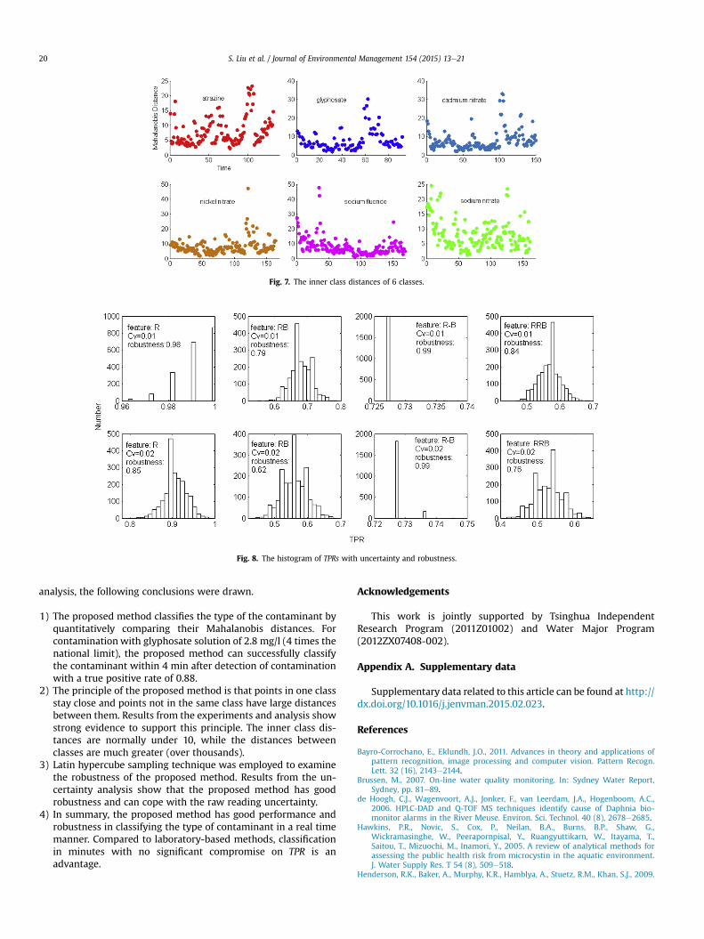
Fig. 7. The inner class distances of 6 classes.

Fig. 8. The histogram of TPRs with uncertainty and robustness.

S. Liu et al. / Journal of Environmental Management 154 (2015) 13e2120

analysis, the following conclusions were drawn.

1) The proposed method classifies the type of the contaminant byquantitatively comparing their Mahalanobis distances. Forcontamination with glyphosate solution of 2.8 mg/l (4 times thenational limit), the proposed method can successfully classifythe contaminant within 4 min after detection of contaminationwith a true positive rate of 0.88.

2) The principle of the proposed method is that points in one classstay close and points not in the same class have large distancesbetween them. Results from the experiments and analysis showstrong evidence to support this principle. The inner class dis-tances are normally under 10, while the distances betweenclasses are much greater (over thousands).

3) Latin hypercube sampling technique was employed to examinethe robustness of the proposed method. Results from the un-certainty analysis show that the proposed method has goodrobustness and can cope with the raw reading uncertainty.

4) In summary, the proposed method has good performance androbustness in classifying the type of contaminant in a real timemanner. Compared to laboratory-based methods, classificationin minutes with no significant compromise on TPR is anadvantage.

Acknowledgements

This work is jointly supported by Tsinghua IndependentResearch Program (2011Z01002) and Water Major Program(2012ZX07408-002).

Appendix A. Supplementary data

Supplementary data related to this article can be found at http://dx.doi.org/10.1016/j.jenvman.2015.02.023.

References

Bayro-Corrochano, E., Eklundh, J.O., 2011. Advances in theory and applications ofpattern recognition, image processing and computer vision. Pattern Recogn.Lett. 32 (16), 2143e2144.

Brussen, M., 2007. On-line water quality monitoring. In: Sydney Water Report,Sydney, pp. 81e89.

de Hoogh, C.J., Wagenvoort, A.J., Jonker, F., van Leerdam, J.A., Hogenboom, A.C.,2006. HPLC-DAD and Q-TOF MS techniques identify cause of Daphnia bio-monitor alarms in the River Meuse. Environ. Sci. Technol. 40 (8), 2678e2685.

Hawkins, P.R., Novic, S., Cox, P., Neilan, B.A., Burns, B.P., Shaw, G.,Wickramasinghe, W., Peerapornpisal, Y., Ruangyuttikarn, W., Itayama, T.,Saitou, T., Mizuochi, M., Inamori, Y., 2005. A review of analytical methods forassessing the public health risk from microcystin in the aquatic environment.J. Water Supply Res. T 54 (8), 509e518.

Henderson, R.K., Baker, A., Murphy, K.R., Hamblya, A., Stuetz, R.M., Khan, S.J., 2009.

S. Liu et al. / Journal of Environmental Management 154 (2015) 13e21 21

Fluorescence as a potential monitoring tool for recycled water systems: a re-view. Water Res. 43 (4), 863e881.

Jeon, J., Kim, J.H., Lee, B.C., Kim, S.D., 2008. Development of a new biomonitoringmethod to detect the abnormal activity of Daphnia magna using automatedgrid counter device. Sci. Total Environ. 389 (2e3), 545e556.

Kroll, D., 2006. Securing Our Water Supply: Protecting a Vulnerable Resource.Pennwell, pp. 36e47.

Liu, S., Che, H., Smith, K., Chen, L., 2014. Contamination event detection usingmultiple types of conventional water quality sensors in source water. Environ.Sci. Proc. Imp. 16 (8), 2028e2038.

Liu, S., Che, H., Smith, K., Chen, C., 2015. A method of detecting contaminationevents using multiple conventional water quality sensors. Environ. Monit.Assess. 187 (1), 4189e4199.

Mahalanobis, P.C., 1936. On the generalised distance in statistics. Proc. Natl. Inst. Sci.India 2 (1), 49e55.

Manache, G., Melching, C.S., 2004. Sensitivity analysis of a water-quality modelusing Latin hypercube sampling. J. Water Res. Plan. Man. 130 (3), 232e242.

Marshall, C.P., Leuko, S., Coyle, C.M., Walter, M.R., Burns, B.P., Neilan, B.A., 2007.Carotenoid analysis of halophilic archaea by resonance Raman spectroscopy.Astrobiology 7 (4), 631e643.

Nguyen, K.A., Stewart, R.A., Zhang, H., 2013. An intelligent pattern recognitionmodel to automate the categorisation of residential water end-use events.Environ. Modell. Softw. 47, 108e127.

Shah, N.K., Gemperline, P.J., 1990. Combination of the Mahalanobis distance andresidual variance pattern-recognition techniques for classification of near-infrared reflectance spectra. Anal. Chem. 62 (5), 465e470.

Storey, M.V., van der Gaag, B., Burns, B.P., 2011. Advances in on-line drinking water

quality monitoring and early warning systems. Water Res. 45 (2), 741e747.Tabacchi, M., Asensio, C., Pavon, I., Recuero, M., Mir, J., Artal, M.C., 2013. A statistical

pattern recognition approach for the classification of cooking stages -Theboiling water case. Appl. Acoust. 74 (8), 1022e1032.

Tao, T., Lu, Y.J., Fu, X., Xin, K.L., 2012. Identification of sources of pollution andcontamination in water distribution networks based on pattern recognition.J. Zhejiang Univ. Sci. A 13 (7), 559e570.

USEPA, 2003. Planning for and Responding to Drinking Water ContaminationThreats and Incidents. Washington, DC, EPA 817-D-04e001.

USEPA, 2005. Water Sentinel System Architecture. U.S. Environmental ProtectionAgency, Office of Water, Office of Ground Water and Drinking Water, Wash-ington, DC. EPA 817-D-05e003.

USEPA, 2008. Water Security Initiative Cincinnati Pilot Post Implementation SystemStatus: Covering the Pilot Period: December 2005 through December 2007. U.S.Environmental Protection Agency, Office of Water, Office of Ground Water andDrinking Water, Washington, DC. EPA 817-R-08e004.

van der Gaag, B., Volz, J., 2008. Real-time On-line Monitoring of Contaminants inWater: Developing a Research Strategy from Utility Experiences and Needs.KIWA Water Research, Nieuwegein.

Wang, C., Feng, Y.J., Zhao, S.S., Li, B.L., 2012. A dynamic contaminant fate model oforganic compound: a case study of nitrobenzene pollution in Songhua River,China. Chemosphere 88 (1), 69e76.

Yang, Y.J., Haught, R.C., Goodrich, J.A., 2009. Real-time contaminant detection andclassification in a drinking water pipe using conventional water quality sensors:techniques and experimental results. J. Environ. Manage. 90 (8), 2494e2506.

Zhao, Z.P., Li, P., Xu, X.Z., 2013. Forecasting model of coal mine water inrush basedon extreme learning machine. Appl. Math. Inf. Sci. 7 (3), 1243e1250.