Embed Size (px)
Citation preview
DM#12494522
2015/16 Price List Information
ELECTRICITY NETWORKS CORPORATION
(“WESTERN POWER”)
ABN 18 540 492 861

Price List Information April 2015
Table of contents
1 Introduction 3
1.1 Code Requirements 3
1.2 2015/16 Foreword 3
1.3 Revenue requirement for 2015/16 6
1.4 Forecast revenue recovery 8
1.5 History of the Tariffs 9
2 Pricing Principles Overview 10
2.1 Pricing Objectives 10
2.2 Pricing Principles 10
2.3 Pricing Methods 11
3 Derivation of Transmission System Cost of Supply 14
3.1 Cost Pools 14
3.2 Cost of Supply 15
3.3 Methodology of Allocating to Cost Pools 18
3.4 Cost Pool Allocations 19
4 Derivation of Distribution System Cost of Supply 20
4.1 Cost Pools 20
4.2 Customer Groups 20
4.3 Locational Zones 20
4.4 Methodology of Deriving the Cost of Supply 22
4.5 Cost Pool Allocations 27
5 Reference Tariff Structure 29
5.1 Reference Services and Tariff Structure 29
5.2 Exit Service Tariff Overview 29
5.3 Entry Service Tariff Overview 32
5.4 Bi-directional Service Tariff Overview 33
6 Derivation of Transmission System Tariff Components 34
6.1 Cost Reflective Network Pricing 34
DM#12494522 i

Price List Information April 2015
6.2 Price Setting for Transmission Reference Services 35
6.3 Price Setting for Distribution Reference Services 38
6.4 Annual Price Review 45
7 Derivation of Distribution System Tariff Components 46
7.1 Price Setting 46
7.2 Demonstration of Derivation of Distribution Components of Distribution Reference Tariffs 53
7.3 Demonstration that Distribution Reference Tariffs are between incremental and stand-alone cost of service provision 57
7.4 Demonstration that incremental costs are recovered through variable components 58
7.5 Annual Price Review 58
7.6 Tariff Equalisation Contribution (TEC) in the Distribution Components of Distribution Reference Tariffs 58
8 Price Changes 62
8.1 Side constraint demonstration 62
8.2 Re-balancing of tariffs 63
8.3 Individual component changes 64
Appendix A - Price Setting for New Transmission Nodes Policy 76
DM#12494522 ii
1
Price List Information April 2015
Introduction This document is Western Power’s Price List Information, as defined in the Electricity Networks Access Code 2004 (the Code), to apply from 1 July 2015.
This document details:
• The history of the network tariffs;
• The Price List’s compliance with the Access Arrangement;
• The objectives and principles that underlie Western Power’s approach to deriving the reference tariffs; and
• The methodology of deriving cost of supply and the reference tariffs from the target revenue.
1.1 Code Requirements Section 8.1 of the Code requires Western Power to submit Price List Information to the Economic Regulation Authority (the Authority).
The Code defines Price List Information as:
“price list information” means a document which sets out information which would reasonably be required to enable the Authority, users and applicants to:
(a) understand how the service provider derived the elements of the proposed price list; and
(b) assess the compliance of the proposed price list with the access arrangement.
The access arrangement specifies the revenue cap form of price control and details the revenue that Western Power is able to earn in each year of the access arrangement period. The access arrangement contains the detailed price control formula that is applied each year to determine the network tariffs. Network tariffs are set each year to recover no more than the revenue cap. The revenue cap is the sum of:
• Western Power’s revenue requirement contained in the access arrangement, plus
• an adjustment for any previous year revenue over or under-recoveries (known as the k-factor adjustment), plus
• an adjustment for the Tariff Equalisation Contribution (TEC).
The access arrangement requires Western Power to seek the Authority’s approval each year for the price list.
1.2 2015/16 Foreword
This section details a number of matters that relate specifically to the preparation of the 2015/16 Price List.
1.2.1 Tariff revenue recovered in 2014/15
Western Power expects to recover $1,388 million from revenue cap services during 2013/14. This is an $18 million under-recovery against the revenue target.
DM#12494522 3

Price List Information April 2015
Table 1 shows the expected revenue compared with the forecast revenue over 2014/15 on a tariff by tariff basis. It shows that the biggest revenue variances were on RT1 and RT4.
Table 1 – Forecast revenue compared with expected revenue in 2014/15 ($M Nominal)
2014/15 Price List forecast F2 forecast
GWh Customer Numbers
Forecast Revenue
GWh Customer Numbers
Expected Revenue
TRT1 – Transmission Exit N/A 26 35.3 N/A 32 32.5
TRT2 – Transmission Entry N/A 30 56.2 N/A 38 55.7
RT1 - Anytime Energy (Residential) 4,930 920,862 661.7 4,847 909,357 648.2
RT2 - Anytime Energy (Business) 1,142 84,607 166.5 1,173 92,486 167.6
RT3 - Time of Use Energy (Residential) 152 21,869 18.3 159 21,850 17.7
RT4 - Time of Use Energy (Business) 1,966 15,107 188.1 2,006 14,817 178.8
RT5 - High Voltage Metered Demand 389 128 20.5 367 123 19.9
RT6 - Low Voltage Metered Demand 1,701 2,187 103.5 1,642 1,860 111.9
RT7 - High Voltage Contract Maximum Demand 3,135 276 96.5 3,077 271 100.2
RT8 - Low Voltage Contract Maximum Demand 231 60 12.4 227 60 13.0
RT9 – Streetlighting 125 255,346 35.8 123 251,114 35.7
RT10 - Unmetered Supplies 33 15,814 3.9 33 15,900 3.9
RT11 - Distribution Entry 0 20 2.8 N/A 23 3.3
RT13 – Anytime Energy (Residential) Bi-directional
Service
0 0 0 0 0 0
RT14 – Anytime Energy (Business) Bi-directional
Service
0 0 0 0 0 0
RT15 – Time of Use (Residential) Bi-directional
Service
0 0 0 0 0 0
RT16 – Time of Use (Business) Bi-directional
Service
0 0 0 0 0 0
Total Reference Service Revenue 13,804 1,316,332 1,402 13,654 1,298,610 1,388
Standby - - 4
TOTAL REVENUE CAP REVENUE 1,406 1,298,610 1,388
In addition to the expected under recovery in 2014/15, Western Power had intentionally not recovered $27 million as part of the 2014/15 Price List in order to avoid price shock. This has been factored into the calculation of the 2015/16 correction factor.
1.2.2 Growth forecasts for 2015/16
The 2015/16 Price List is based on Western Power’s most recent forecasts of energy consumption and customer numbers (prepared in March 2015). Energy consumption and customer number forecasts are important because they are used to divide the overall revenue requirement across customers and into a price per unit of energy sold.
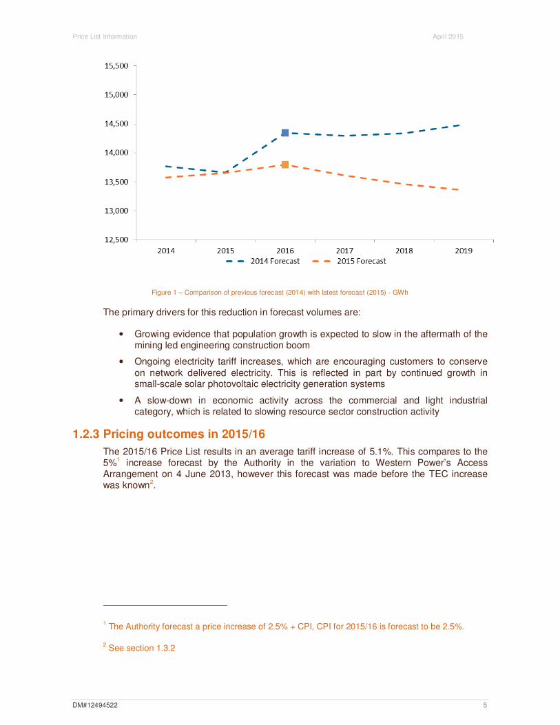
The energy forecasts for the 2015/16 price list were produced using the latest available customer data and other economic inputs. The resulting forecast is again lower than Western Power’s previous forecasts. This outcome is consistent with what is occurring in other jurisdictions across Australia. The chart below highlights the differences in energy volumes over the forecast period.
DM#12494522 4
Price List Information April 2015
Figure 1 – Comparison of previous forecast (2014) with latest forecast (2015) - GWh
The primary drivers for this reduction in forecast volumes are:
• Growing evidence that population growth is expected to slow in the aftermath of the mining led engineering construction boom
• Ongoing electricity tariff increases, which are encouraging customers to conserve on network delivered electricity. This is reflected in part by continued growth in small-scale solar photovoltaic electricity generation systems
• A slow-down in economic activity across the commercial and light industrial category, which is related to slowing resource sector construction activity
1.2.3 Pricing outcomes in 2015/16
The 2015/16 Price List results in an average tariff increase of 5.1%. This compares to the 5%1 increase forecast by the Authority in the variation to Western Power’s Access Arrangement on 4 June 2013, however this forecast was made before the TEC increase was known2.
1 The Authority forecast a price increase of 2.5% + CPI, CPI for 2015/16 is forecast to be 2.5%.
2 See section 1.3.2
DM#12494522 5
Price List Information April 2015
1.3 Revenue requirement for 2015/16
The following sections detail the calculation of the revenue requirements for Western Power’s Transmission and Distribution networks.
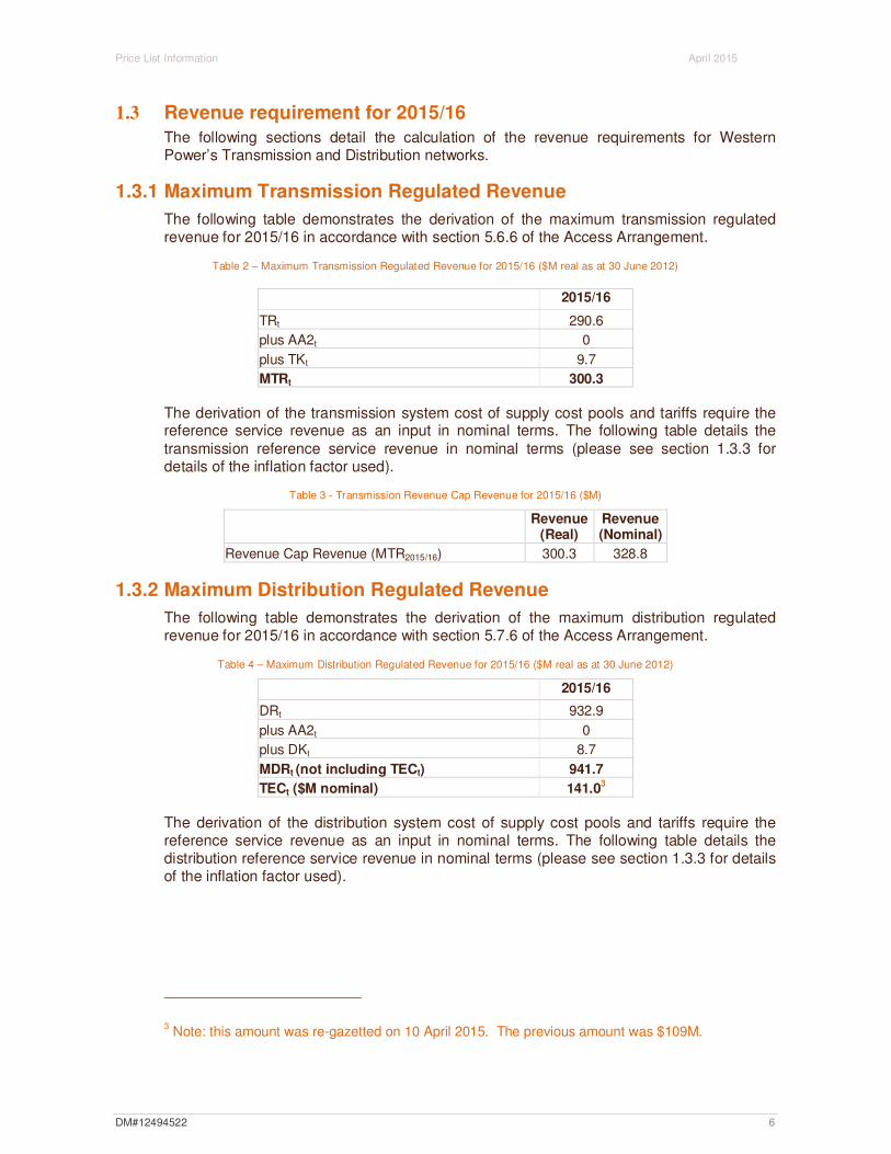
1.3.1 Maximum Transmission Regulated Revenue
The following table demonstrates the derivation of the maximum transmission regulated revenue for 2015/16 in accordance with section 5.6.6 of the Access Arrangement.
Table 2 – Maximum Transmission Regulated Revenue for 2015/16 ($M real as at 30 June 2012)
2015/16
TRt 290.6
plus AA2t 0
plus TKt 9.7
MTRt 300.3
The derivation of the transmission system cost of supply cost pools and tariffs require the reference service revenue as an input in nominal terms. The following table details the transmission reference service revenue in nominal terms (please see section 1.3.3 for details of the inflation factor used).
Table 3 - Transmission Revenue Cap Revenue for 2015/16 ($M)
Revenue (Real)
Revenue (Nominal)
Revenue Cap Revenue (MTR2015/16) 300.3 328.8
1.3.2 Maximum Distribution Regulated Revenue
The following table demonstrates the derivation of the maximum distribution regulated revenue for 2015/16 in accordance with section 5.7.6 of the Access Arrangement.
Table 4 – Maximum Distribution Regulated Revenue for 2015/16 ($M real as at 30 June 2012)
2015/16
DRt 932.9
plus AA2t 0
plus DKt 8.7
MDRt (not including TECt) 941.7
TECt ($M nominal) 141.03
The derivation of the distribution system cost of supply cost pools and tariffs require the reference service revenue as an input in nominal terms. The following table details the distribution reference service revenue in nominal terms (please see section 1.3.3 for details of the inflation factor used).
3 Note: this amount was re-gazetted on 10 April 2015. The previous amount was $109M.
DM#12494522 6

Price List Information April 2015
Table 5 - Distribution Revenue Cap Revenue for 2015/16 ($M)
Revenue (Real)
Revenue (Nominal)
MDRt (not including TECt) 941.7 1,031.0
Revenue Cap Revenue (MDR2015/16) 1,172.0
1.3.3 Derivation of Inflation Factor
In sections 1.3.1 and 1.4.2 Western Power has inflated the reference service revenue from real terms to nominal terms by using real and forecast inflation in accordance with sections 5.6.6 and 5.7.6 of the Access Arrangement.
Table 6 - Derivation of 2015/16 Inflation Factor
December 2011 – December 2012 – Actual 2.20%
December 2012 – December 2013 – Actual 2.75%
December 2013 – December 2014 – Actual 1.72%
December 2014 – December 2015 – Forecast 2.50%
Derived Inflation Factor 1.095
DM#12494522 7

Price List Information April 2015
1.4 Forecast revenue recovery
The following table sets out the reference service revenue, by tariff, which is forecast to be collected when applying the 2015/16 Price List.
Table 7 – Reference Service Revenue Forecast in 2015/16 ($M Nominal)
kWh Customer Numbers
Forecast Transmission
Revenue Recovered
Forecast Distribution
Revenue Recovered
TRT1 – Transmission Exit N/A 28 35.3 0.0
TRT2 – Transmission Entry N/A 30 51.7 0.0
RT1 - Anytime Energy (Residential) 5,040,980,245 927,656 84.4 636.7
RT2 - Anytime Energy (Business) 1,180,341,029 85,671 23.5 154.8
RT3 - Time of Use Energy (Residential) 159,278,898 21,594 2.6 17.0
RT4 - Time of Use Energy (Business) 1,963,747,971 14,951 38.2 164.7
RT5 - High Voltage Metered Demand 363,429,118 132 5.1 14.7
RT6 - Low Voltage Metered Demand 1,642,782,344 2,479 25.4 82.2
RT7 - High Voltage Contract Maximum Demand 3,066,884,986 285 51.9 48.9
RT8 - Low Voltage Contract Maximum Demand 223,356,447 61 4.0 9.1
RT9 – Streetlighting 123,353,806 248,492 1.3 37.0
RT10 - Unmetered Supplies 32,680,258 15,531 0.2 4.1
RT11 - Distribution Entry 0 20 1.3 2.0
RT13 – Anytime Energy (Residential) Bi
directional Service
0 0 0 0
RT14 – Anytime Energy (Business) Bi
directional Service
0 0 0 0
RT15 – Time of Use (Residential) Bi-directional
Service
0 0 0 0
RT16 – Time of Use (Business) Bi-directional
Service
0 0 0 0
Total Reference Service Revenue 13,796,835,102 1,316,930 324.9 1,171.3
Standby Services - - 3.9 0.7
TOTAL REVENUE CAP REVENUE 328.8 1,172.01
Over/(Under) recovery compared to
maximum transmission/distribution
regulated revenue
- -
DM#12494522 8

Price List Information April 2015
1.5 History of the Tariffs
Prior to the commencement of the Code and the first Access Arrangement Western Power had in place a suite of tariffs to recover the regulated revenue for both the transmission and distribution network businesses.
Network tariffs have been in place since the introduction of de-regulation into the southwest electricity network in 1996. Initially tariffs were only determined and published for contestable users but from July 2001 network tariffs were established for all users whether contestable or franchise.
In July 2001 the network tariff structure changed somewhat from the structure in place before 2001. This became necessary to improve the efficiency of the tariff structure and to cater, in particular, for the smaller contestable and non-contestable users. Prior to 2001 the transmission and distribution access price structures were entirely different and users seeking access to the networks had separate transmission and distribution access contracts and paid separate charges. However, a full review of the tariff structures was performed resulting in separate transmission and distribution tariffs which may be added together to form a single bundled tariff for distribution connected users. However, the transmission and distribution tariffs are still separately determined.
With the exception of the introduction of bi-directional tariffs at the commencement of AA3, Western Power has maintained the remaining network tariff structure for the reference services offered under the Access Arrangement since its commencement on 1 July 2006.
DM#12494522 9

2
Price List Information April 2015
Pricing Principles Overview This section discusses the principles, objectives and an overview of the methodology used in determining the reference tariffs.
2.1 Pricing Objectives
Reference service revenue is recovered through a set of reference tariffs that have been designed to meet high-level objectives described below.
Note: Transmission and distribution are treated separately and each has independent target revenue for reference services.
The reference service revenue is recovered from users in a manner that is:
• Economically efficient;
• Transparent;
• Practical; and
• Equitable.
In addition to these objectives, the pricing methodology is developed to:
• Achieve the reference service revenue to maintain a viable network business and to deliver efficient network services to all network users;
• Be as cost reflective as is reasonable to reflect the network user’s utilisation of the network including use of dedicated assets;
• Promote efficient use of the network through appropriate price signalling;
• Maintain price stability and certainty to enable network users to make informed investment decisions;
• Be as simple and straightforward as is reasonable taking into account other objectives; and
• Avoid cross subsidy between different user groups where possible. From an economic efficiency perspective this requires that the reference tariff be between the incremental cost of supply and the stand-alone cost of supply.
2.2 Pricing Principles
Western Power has adopted the following principles that are designed to meet the pricing objectives set out in the previous section.
1. Tariffs are designed to recover the revenue cap revenue entitlement within the side constraints to prevent price shock to users.
2. The prices are based on a well-defined and transparent methodology.
3. The prices are based on analysis of the cost of supply provision that includes:
a. Definition of the classes of service provided;
b. Allocation of fixed and variable network costs to service classes; and
c. Price setting to recover the fixed and variable costs.
4. Prices signal the economic cost of supply provision in that they:
DM#12494522 10

Price List Information April 2015
a. Avoid cross subsidies between classes of service; and
b. Avoid cross subsidies between customers within each class of service.
5. Provided that economic costs are covered, prices are responsive to user requirements in order to:
a. Avoid economic bypass; and
b. Allow for negotiation where provided within the Code.
6. Provide economic signals to encourage efficient use of the network.
7. Reference tariffs for users with annual energy demand below 1 MVA are uniform (consistent with the section 7.7 of the Code), but will meet the pricing principles described above, as far as is practical.
2.3 Pricing Methods
The pricing methods (cost allocations) are set out in section 6.5 of the Access Arrangement. This section provides a summary of Western Power’s pricing methods.
2.3.1 General
Reference tariffs aim to reasonably reflect the cost of providing the network service to users. The first step in developing reference tariffs is to model the cost of supply for users. The cost of supply cannot be derived at an individual user level and so users are categorised into a number of groups with similar costs.
Reference tariffs will generally have a number of components, which fall into fixed and variable categories. Fixed components would generally be a charge per user regardless of their size whereas the variable component would be related to energy or demand. These categories of costs reflect the fact that costs will be related either to the number of users serviced or to the amount of capacity provided.
The two processes of “determining cost of supply” and “setting reference tariffs” to recover those costs are separate so that the costs of supply can be allocated to particular customer groups and the reference tariffs can be set to recover those costs. The costs are separated into fixed and variable components and the reference tariffs are similarly split so that fixed costs are recovered by fixed charges and variable costs by variable charges.
It is recognised that the determination of the cost of supply for users and respective reference tariffs is an inexact process. A number of simplifying assumptions are required, for example, to categorise users into a small number of customer groups or classes with similar characteristics.
It is also noted that demand is the best measurement of capacity. However, the vast majority of users have energy only metering (or no metering at all) that does not record demand, and therefore energy is used as a proxy for demand.
2.3.2 Process to Determine Cost of Supply
This section presents an overview of the process to derive the cost of supply. Detailed information on this process is provided in sections 3 and 4.
There are two basic stages in determining the cost of supply for users:
• Determination of the reference service revenue for Western Power; and
DM#12494522 11

Price List Information April 2015
• Allocation of the revenue components to different cost pools for various customer groups, based on factors such as supply voltage, location and load characteristics.
Note: Transmission and distribution are treated separately and each has independent target revenues.
The reference service revenue requirement must then be allocated to asset classes and the use of the assets allocated to users. The customer groups used in the analysis and modelling of costs generally reflect the nature of the physical connection to the network and the relative size and nature of the user, namely:
Transmission connected:
� Transmission Generation
� Transmission Loads
Distribution connected:
� High Voltage >1 MVA maximum demand
� High Voltage <1 MVA maximum demand
� Low Voltage >1 MVA maximum demand
� General Business Large (300-1,000 kVA maximum demand)
� General Business Medium (100-300 kVA maximum demand)
� General Business Small (15-100 kVA maximum demand)
� Small Business (<15 kVA maximum demand)
� Residential
� Streetlights
� Unmetered Supplies
2.3.3 Process to Determine Reference Tariffs
This section presents an overview of the process by which reference tariffs are derived. Detailed information on the process is provided in sections 6 and 7.
The users within the customer groups are linked to reference tariffs so that cost of supply can then be derived for each reference tariff. The cost of supply is in terms of fixed and variable costs and price settings are then simply established to recover the cost pools from the users.
2.3.4 Modelling Cost Allocations
Western Power’s transmission and distribution cost of supply (COS) models accurately reflect the network cost of supply for the various customer groups. The model assembles capital and operating costs for the components (lines, substations, transformers, etc.) of the
DM#12494522 12

Price List Information April 2015
modern equivalent assets employed in providing network capacity and delivering energy and allocates these to each customer group according to a pre-determined set of principles.
Tables from Western Power’s COS model are provided in this document to demonstrate that Western Power complies with its cost allocation methodology.
DM#12494522 13

Price List Information April 2015
3 Derivation of Transmission System Cost of Supply This section details the derivation of the transmission system cost of supply for connection points on the transmission system.
3.1 Cost Pools
The following cost pools are used in the derivation of the transmission system cost of supply:
• Connection Services Cost Pool. Which is further allocated to the following cost pools:
• Connection Services for Exit Points Cost Pool; and
• Connection Services for Entry Points Cost Pool.
• Shared Network Services Cost Pool. Which is further allocated to the following cost pools:
• Use Of System for Loads Cost Pool;
• Use Of System for Generators Cost Pool; and
• Common Service for Loads Cost Pool.
• Control System Services Cost Pool. Which is further allocated to the following cost pools:
• Control System Services for Loads Cost Pool; and
• Control System Services for Generators Cost Pool.
3.1.1 Connection Services for Exit Points Cost Pool
The Connection Services for Exit Points Cost Pool includes the Gross Optimised Deprival Value (GODV) of all connection assets at each Exit Point and one-third of the value of the voltage control assets at those points (since the function of voltage control equipment is partly location specific and partly system related).
3.1.2 Connection Services for Entry Points Cost Pool
The Connection Services for Entry Points Cost Pool includes the GODV of all connection assets at each Entry Point and one-third of the value of the voltage control assets at those points (since the function of voltage control equipment is partly location specific and partly system related).
3.1.3 Use of System for Loads Cost Pool
Use of System for Exit Points Cost Pool includes 50% of the total Shared Network Services Cost Pool.
3.1.4 Use of System for Generators Cost Pool
Use of System for Entry Points Cost Pool includes 20% of the total Shared Network Services Cost Pool.
DM#12494522 14
Price List Information April 2015
3.1.5 Common Service for Loads Cost Pool
The Common Service for Loads Cost Pool includes:
• 30% of the total Shared Network Services Cost Pool;
• Shared Voltage Control Assets – two thirds of the value of voltage control assets at Entry and Exit points (since the function of voltage control equipment is partly location specific and partly system related) and the value of all of voltage control assets at transmission substations; and
• Adjustments for under or over recovery of revenue expected for any reason in any other tariff component.
3.1.6 Control System Service for Loads Cost Pool
The Control System Service for Loads Cost Pool consists of a portion of the total cost of all SCADA, SCADA related communications equipment, and costs associated with the control centre, proportioned based on the total number of points in the SCADA master station relevant to loads.
3.1.7 Control System Service for Generators Cost Pool
The Control System Service for Generators Cost Pool consists of a portion of the total cost of all SCADA, SCADA related communications equipment, and costs associated with the control centre, proportioned based on the total number of points in the SCADA master station relevant to generators.
3.2 Cost of Supply
In order to calculate transmission cost of supply, all transmission assets are valued and categorised into the above cost pools. Each network branch is further defined as either exit, entry or shared network and cost allocation is then applied based on the GODV of all relevant assets.
3.2.1 Transmission Assets
The principal elements of the transmission networks include transmission substations and zone substations, interconnected by transmission and sub-transmission lines. The transmission networks enable the transportation of electricity from power stations to zone substations and high voltage user loads. The zone substations provide the interface between the transmission networks and distribution networks.
Generally, the transmission networks assets comprise connection assets, shared network assets and other or ancillary assets. These are described as follows:
• Connection Assets: those assets at the point of physical interconnection with the transmission networks which are dedicated to a User - that is, at substations including transformers and switchgear, but excluding the incoming line switchgear. Connection assets for generators are referred to as entry assets and for loads they are called exit assets.
• Shared Network Assets: all other transmission assets, which are shared to some extent by network Users.
DM#12494522 15

Price List Information April 2015
• Other or Ancillary Assets: network assets performing an Ancillary Services function comprise:
• those providing a Control System Service, for example, system control centres, supervisory control and communications facilities.
• those providing a Voltage Control Service in the networks, for example, a proportion of the costs of capacitor and reactor banks in substations.
Figure 2 shows, in simplified form, the principal elements of the transmission networks and the categorisation of the assets as described above.
DM#12494522 16

NET
Price List Information April 2015
Transmission Network Assets
Generator
Transformer
330,220 & 132 kV
132 & 66 kV Lines
POWER STATION
SHARED
CONNECTION ASSETS (EXIT)
CONNECTION ASSETS
ZONE/CUSTOMER SUBSTATIONS
TRANSMISSION SUBSTATION
TRANSMISSION SUBSTATION
Voltage Control Asset
Figure 2 - Transmission Network Assets
DM#12494522 17
Price List Information April 2015
3.2.2 Asset Valuation
All valuations of transmission assets are performed using the Optimised Deprival Value (ODV) methodology.
3.2.3 Valuation of Individual Branches and Nodes
To determine cost of supply, valuation data is required for every individual branch and node on the network. Every branch and node consists of many individual asset valuation building blocks that are all individually assessed.
Branches include transmission lines and transformers and include the substation circuits at each end. Each transmission line branch will typically have the cost of each of the circuit breakers at different substations included, whereas each transformer branch will typically have the cost of each of the circuit breakers at that same substation included.
Substation site establishment costs are allocated equally to all substation circuits.
The costs for shared circuit breakers (such as bus section breakers etc.) are allocated equally between all other substation circuits, which derive benefit from that shared circuit breaker.
3.3 Methodology of Allocating to Cost Pools
3.3.1 Overview
The methodology for allocating the transmission revenue to each cost pool is to allocate the revenue in the proportion to the GODV of the assets in each cost pool.
However, the Annual Revenue Requirement for the Control System Service Cost Pool is calculated separately (using the same method as for all other network assets) but assuming higher depreciation and operating expenditure than for other network assets. When calculating other Cost Pool Revenues appropriate adjustments are required.
Consequently:
Cost Pool Revenue = RR * GODV (Cost Pool)
where:
RR = a revenue rate of return determined as AARRnetwork / ΣGODVnetwork
AARRnetwork = Transmission Reference Service Revenue excluding Annual Revenue Requirement for Control System Services.
GODV (Cost Pool) = GODV of the transmission network assets which belong in that cost pool.
ΣGODVnetwork = GODV of all transmission assets excluding Control System Service assets.
DM#12494522 18
Price List Information April 2015
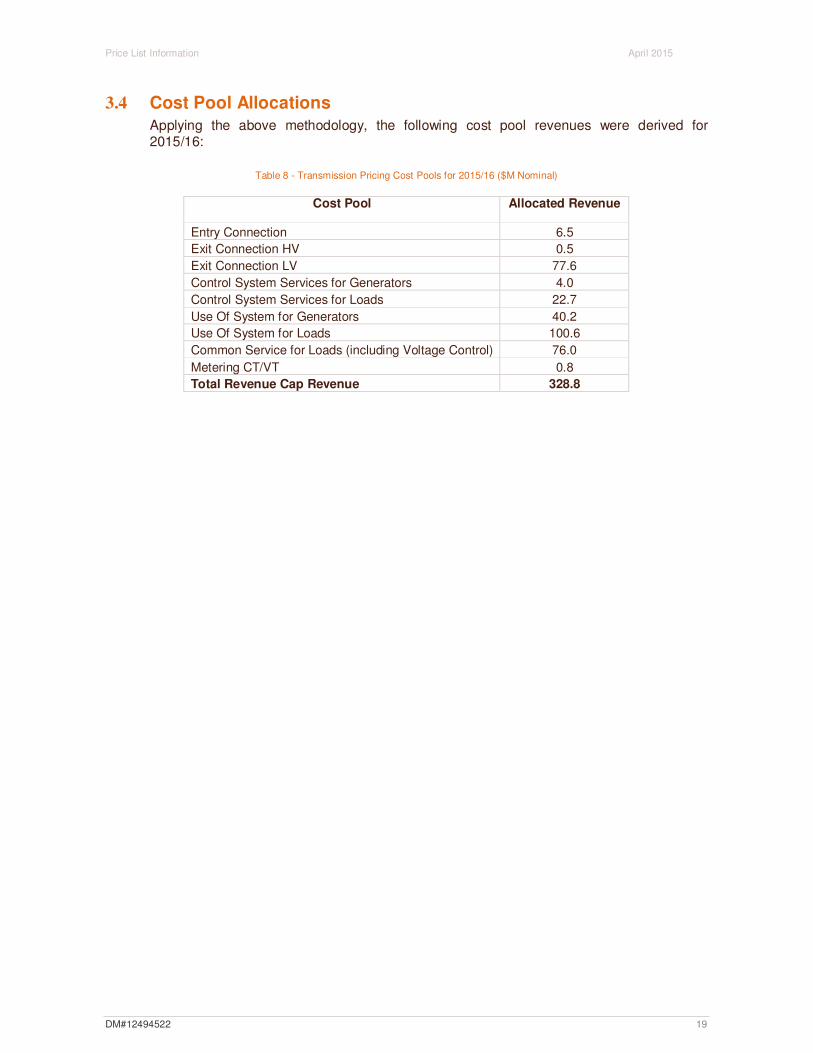
3.4 Cost Pool Allocations
Applying the above methodology, the following cost pool revenues were derived for 2015/16:
Table 8 - Transmission Pricing Cost Pools for 2015/16 ($M Nominal)
Cost Pool Allocated Revenue
Entry Connection 6.5
Exit Connection HV 0.5
Exit Connection LV 77.6
Control System Services for Generators 4.0
Control System Services for Loads 22.7
Use Of System for Generators 40.2
Use Of System for Loads 100.6
Common Service for Loads (including Voltage Control) 76.0
Metering CT/VT 0.8
Total Revenue Cap Revenue 328.8
DM#12494522 19

Price List Information April 2015
4 Derivation of Distribution System Cost of Supply This section details the derivation of the distribution system cost of supply for connection points on the distribution system.
The derivation of the Distribution System Cost of Supply operates along the same principles as the transmission system. That is, the reference service revenue entitlement (which includes the Tariff Equalisation Contribution) is determined for the distribution system, and that revenue is then allocated to asset categories to derive the cost of supply for each of the customer groups. The cost of supply is based on the relative usage of each asset category by the various customer groups.
The structure of the distribution network cost of supply and reference tariffs reflects the features of the distribution network.
4.1 Cost Pools
The distribution cost pools used in the Distribution System Cost of Supply are:
• High Voltage Network
• Low Voltage Network
• Transformers
• Streetlight Assets
• Metering
• Administration
4.2 Customer Groups
The distribution customer groups used in the Distribution System Cost of Supply are:
• High Voltage >1 MVA maximum demand
• High Voltage <1 MVA maximum demand
• Low Voltage >1 MVA maximum demand
• General Business Large (300-1,000 kVA maximum demand)
• General Business Medium (100-300 kVA maximum demand)
• General Business Small (15-100 kVA maximum demand)
• Small Business (<15 kVA maximum demand)
• Residential
• Streetlights
• Unmetered Supplies
4.3 Locational Zones
Distribution reference tariffs are provided for individual locational zones for users with energy demands in excess of 1 MVA. Locational zones are defined as those areas supplied by the network where the distribution system cost of supply is similar. For example, the rural wheat belt areas of Western Australia are considered to have a reasonably uniform distribution system and costs of supply, as do the urban and CBD areas of Perth.
DM#12494522 20
Price List Information April 2015
Zone substations with similar cost structures are allocated to locational zones that feed an area of the distribution system. Where a zone substation supplies an area of more than one distinct cost of supply, then all users supplied from that substation are considered to be in the one dominant category. That is, there is only one locational zone defined for each zone substation.
The five zones are defined in the sections below, and for details of the allocation of each zone substation to locational zones see the Price List in the Access Arrangement.
4.3.1 CBD Locational Zone
This is defined as the intense business area generally recognised as the Perth CBD area. The defining street boundaries is generally from the Swan River north to Aberdeen Street Northbridge, west to Rokeby Road Subiaco, and east to the East Perth redevelopment area.
4.3.2 Urban Locational Zone
This is defined as the uniformly and continuously settled areas of Perth that contains the urban domestic, commercial and industrial users but exclude the CBD. This area also excludes the outer urban area that is treated as mixed. The country towns of Geraldton and Kalgoorlie are also included.
4.3.3 Rural Locational Zone
This is defined to include those areas which have a predominantly rural/farming characteristic and includes small to medium size towns within the southwest land division, for example Merredin.
4.3.4 Mixed Locational Zone
This is defined to include those areas that have a mixed user base that has at least two dominant load types, for example a mix of significant mining and rural loads or significant urban and rural loads. It also includes significant outer areas of Perth, which can be a mix of fringe urban, semi-rural and rural types, for example Yanchep.
4.3.5 Mining Locational Zone
This is defined to include the mining area surrounding Kalgoorlie, which is supplied at 33 kV and the mining area at Forrestania which is also supplied at 33 kV. It does not include the town of Kalgoorlie (Urban zone).
DM#12494522 21

Price List Information April 2015
4.4 Methodology of Deriving the Cost of Supply
4.4.1 Flowchart
The derivation of the cost of supply for each customer group the process followed is illustrated in the following flow diagram.
Determine Distribution Reference Service Revenue
Entitlement
Allocate Revenue Entitlement to Cost Pools: HV Network,
Transformers and LV Network
Determine Distribution Revenue Cap Revenue Entitlement
Identify Nonreference Services Revenue
Derive annual Standalone Cost and Minimum Cost of Service
for each HV and LV CMD Customer with demand greater than
1 MVA
Set Zonal CMD HV tariff component so that the HV Network
Revenue Recovered from CMD customers is within the
minimum and standalone cost of service
Determine HV Network Cost Pool to be recovered from all HV
and LV CMD customers by applying the derived prices to the
forecast customer demands
Determine the Residual HV Network Cost Pool that can be
recovered from nonCMD customers
Determine Anytime Maximum Demands for each of the non
CMD customer groups and adjust demands for Loss Factors to
reflect the actual usage of each asset class by each customer
group
Allocate the HV Network, Transformers and LV Network cost
pools to each of the customer groups based on their Loss
Factor adjusted demands
Figure 3 - Distribution Cost of Supply Flow Chart
DM#12494522 22

Price List Information April 2015
Each step in this process to derive the distribution cost of supply is described in more detail in the following sections.
4.4.2 Calculate the Forecast Distribution Network Revenue to be recovered from Distribution-Connected Users
It is assumed at this stage that the forecast distribution network revenue entitlement has been determined in accordance with the approach approved by the Authority in the Access Arrangement.
The forecast distribution network revenue entitlement includes an amount for the TEC. The allocation of TEC to the cost pools and the customer groups is undertaken on the same basis as the network revenue entitlement set out below.
4.4.3 Allocate Revenue Entitlement to Cost Pools HV Network, Transformers and LV Network
The network revenue entitlement is then allocated to each of the asset classes being the HV network, transformers and the LV network. The allocation is based on the GODV of each asset category as a proportion of the total GODV.
4.4.4 Derive HV annual stand-alone cost and incremental cost of supply for all HV and LV CMD users with demand greater than 1 MVA
In the cost of supply analysis, the costs for users with annual maximum demands less than 1,000 kVA are assumed to be uniform across the network whereas costs for users with demands above 1,000 kVA are determined on the basis of their location on the network and relative use of network assets.
On this basis, the HV network costs that can be allocated to users with maximum demands in excess of 1,000 kVA are calculated through a process that ensures that the cost is between the incremental and stand-alone cost of supply. This approach is consistent with the requirements of section 7.3 of the Code and demonstrated in section 7.3.
In terms of costs of supply analysis, this approach is contrary to the approach for users with demands below 1,000 kVA. For these users the approach is facilitated by allocating the network costs on the basis of sharing the average costs of the network between users depending on their relative usage of the network components.
This approach for larger users can distort the final price outcomes because it assumes that costs can be allocated linearly on usage. This approach is reasonable for smaller users where the stand-alone cost will far exceed the average cost of supply. On the other hand, the stand-alone cost for larger users can be less than a simple linear allocation of costs and for this reason it is essential to take a different approach.
The approach taken is to derive the HV network incremental and standalone cost for each user with maximum demand in excess of 1,000 kVA. This process will give maximum and minimum revenues that could be recovered from this customer group.
The reality of network pricing is that the actual revenue recovered from these users should fall between these two values. The actual value is determined by deriving reference tariff components that, when applied to the forecast user data will produce charge and revenue
DM#12494522 23

Price List Information April 2015
outcomes that recover at least the incremental cost of supply but do not recover more than the standalone cost of supply. The detail of this price setting is contained in section 7.
4.4.5 Redefine Revenue Pools
The outcome of the process to date is that the HV network revenue for HV and LV users with maximum demands greater than 1,000 kVA has been forecast. This now results in a reallocation of the reference tariff revenue entitlement into the costs pools of:
• HV network cost pool that is recovered from users with demands greater than 1,000 kVA
• Residual HV network cost pool for users with demands less than 1,000 kVA
• Transformer cost pool
• LV network cost pool
These cost pools must now be allocated to customer groups based on relative usage of the network elements.
4.4.6 Allocation of Residual HV Network Costs to Customer Groups
This allocation is to reflect the usage of each of the customer groups of the HV network remembering that the costs associated with users with maximum demands greater than 1,000 kVA have already been determined.
The allocation is based on the diversified maximum demand imposed by each customer group. Where a user has a metered demand, that demand is recorded but for the vast majority of users there is no metered demand. For all of these users a notional demand is calculated based on their diversified load factor. Those calculated demands are adjusted by average loss factors to reflect the actual demand placed on the HV network.
The load factors are based on industry codes that reflect typical users. These load factors were derived from sample data taken over a large number of users and are recorded against each user. The sum of the demands is called the anytime maximum demand (ATMD).
The loss factors that are used are listed by customer group as follows:
Customer Group Loss Factor (%)
Unmetered 8
Streetlights 8
Residential 8
Small Business 8
General Business Small 8
General Business Medium 5
General Business Large 4
Low Voltage >1MVA 4
High Voltage 1
4.4.7 Fixed and Variable Costs
Based on the premise that the network was built in part to supply each user, it is reasonable to allocate some of the HV costs on a per user basis rather than purely on demand. Capacity to carry load should clearly be allocated on demand, but the cost to get a
DM#12494522 24
Price List Information April 2015
minimum capacity supply to a user should, in principle, simply be allocated on a per user basis. This reflects the principle that all users benefit from the HV line regardless of their actual usage.
The question of what percentage of costs should be allocated on a per user basis is the classical fixed and variable cost allocation issue. To determine the fixed component of the cost the approach taken will be to calculate the cost to establish the network to supply the smallest possible load to each user. The variable component of the cost can then be based on all costs that give the network capacity to provide differential supply to each user. That process is described below.
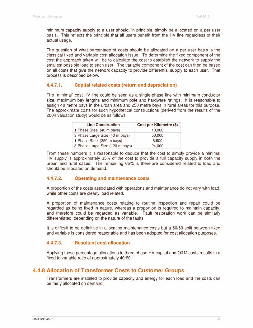
4.4.7.1. Capital related costs (return and depreciation)
The “minimal” cost HV line could be seen as a single-phase line with minimum conductor size, maximum bay lengths and minimum pole and hardware ratings. It is reasonable to assign 40 metre bays in the urban area and 250 metre bays in rural areas for this purpose. The approximate costs for such hypothetical constructions (derived from the results of the 2004 valuation study) would be as follows.
Line Construction Cost per Kilometre ($)
1 Phase Steel (40 m bays) 18,000
3 Phase Large Size (40 m bays) 50,000
1 Phase Steel (250 m bays) 8,500
3 Phase Large Size (120 m bays) 24,000
From these numbers it is reasonable to deduce that the cost to simply provide a minimal HV supply is approximately 35% of the cost to provide a full capacity supply in both the urban and rural cases. The remaining 65% is therefore considered related to load and should be allocated on demand.
4.4.7.2. Operating and maintenance costs
A proportion of the costs associated with operations and maintenance do not vary with load, while other costs are clearly load related.
A proportion of maintenance costs relating to routine inspection and repair could be regarded as being fixed in nature, whereas a proportion is required to maintain capacity, and therefore could be regarded as variable. Fault restoration work can be similarly differentiated, depending on the nature of the faults.
It is difficult to be definitive in allocating maintenance costs but a 50/50 split between fixed and variable is considered reasonable and has been adopted for cost allocation purposes.
4.4.7.3. Resultant cost allocation
Applying these percentage allocations to three phase HV capital and O&M costs results in a fixed to variable ratio of approximately 40:60.
4.4.8 Allocation of Transformer Costs to Customer Groups
Transformers are installed to provide capacity and energy for each load and the costs can be fairly allocated on demand.
DM#12494522 25

Price List Information April 2015
The cost of maintenance of transformers is a very small proportion of the total distribution network maintenance expense, and so no maintenance costs are allocated to transformers.
4.4.9 Allocation of LV Network Costs to Customer Groups
The logic for developing cost allocation principles for LV network costs is identical to the HV case. Therefore, the LV costs are allocated on a similar basis.
However, the LV costs per kVA are generally higher for smaller users than for larger users. Larger users use proportionately less of the LV network because they are typically connected closer to transformers, and generally have a lower level of back-up. For example, a user with a load of 300 kVA or more would generally be connected directly to a transformer with limited capacity in the LV network to supply only part load in the event of an HV contingency.
Appropriate weighting factors have therefore been derived to reflect the proportionate usage of the LV network by the different customer groups, as follows:
Customer Group Cost Weighting
Residential 1
Small business 1
General business - small 1
General business - medium 0.9
General business - large 0.1
Low Voltage >1,000 kVA 0.1
High Voltage 0
4.4.10 Allocation of Tariff Equalisation Contribution (TEC) Costs to Customer Groups
TEC is allocated to the cost pools consistent with the methodology detailed above. TEC is then allocated to customers groups on the same basis that is set out above for:
1. Allocation of HV Network Costs to customer groups
2. Allocation of Transformer Costs to customer groups
3. Allocation of LV Network Costs to customer groups
4.4.11 Streetlighting Costs
Allocation of network costs to streetlighting is in two components - the use of network costs and the costs associated with the streetlight asset itself.
4.4.11.1. Use of Network Costs
Costs for the use of the HV and LV networks and transformers are allocated on a fixed and variable basis as for other customer groups, but with customer numbers reduced by a factor of 10.
4.4.11.2. Streetlight Asset Costs
The allocation of the streetlight asset costs is based on the average cost per light, as derived in the asset valuation, applied over the total asset.
DM#12494522 26

Price List Information April 2015
4.4.12 Metering Costs
Metering costs are determined from asset information for the various customer groups and both capital and maintenance costs are allocated on a per user basis across each group.
4.4.13 Administration Costs
The allocation of administration costs is based on specific charges for the larger customer groups, with the residual cost pool allocated by ATMD over the other customer groups.
4.5 Cost Pool Allocations
Applying the above methodology, the following tables detail the allocation of the distribution network revenue entitlement (which includes TEC) to the cost pools and customer groups:
Table 9 - Distribution Cost Pools for 2015/16 ($M Nominal)
Locational Zone
Cost Pool CBD Urban Goldfields
Mining Mixed Rural Total
High Voltage Network 11.9 179.4 4.0 118.5 120.9 434.8
High Voltage Network > 1,000 kVA 8.6 33.2 5.3 10.8 2.7 60.6
High Voltage Network Total 20.5 212.6 9.3 129.3 123.6 495.4
Low Voltage Network 11.4 184.3 1.5 47.3 17.8 262.3
Transformers 7.8 78.2 2.1 36.0 23.2 147.2
Streetlight Assets 26.7
Metering 68.3
Administration 172.1
Revenue requirement 1,172.0
DM#12494522 27

Price List Information April 2015
Table 10 - Distribution Reference Service Customer Groups for 2015/16 ($M Nominal)
Hig
h V
olt
ag
e N
etw
ork
Lo
w V
olt
ag
e N
etw
ork
Tra
ns
form
ers
Str
eetl
igh
t A
ssets
Mete
rin
g
Ad
min
istr
ati
on
AT
MD
MV
A
GW
h
Lo
ss
Ad
jus
ted
AT
MD
's
Tra
ns
form
er
Ad
jus
ted
AT
MD
's
LV
Ad
juste
d A
TM
D's
Nu
mb
er
of
Cu
sto
mers
LV
Ad
jus
ted
Cu
sto
mer
Nu
mb
ers
Fix
ed
$/a
nn
um
Vari
ab
le $
/an
nu
m
Fix
ed
$/a
nn
um
Vari
ab
le $
/an
nu
m
Vari
ab
le $
/an
nu
m
Fix
ed
Unmetereds 5 33 6 6 6 15,531 15,531 1.9 0.3 1.3 0.3 0.2 0.0 0.0 0.6
Streetlights 30 123 33 33 3 248,492 24,849 3.6 2.0 1.9 0.2 1.0 26.7 0.0 1.6
Residential 2,035 5,200 2,205 2,205 2,205 949,250 949,250 121.8 128.3 73.9 100.8 67.6 0.0 51.3 91.1
Small Business 466 1,115 487 487 487 86,445 86,445 18.1 34.3 6.8 22.2 16.4 0.0 9.1 17.6
General Business - Small 590 1,187 617 617 617 12,963 12,963 2.2 41.1 1.1 28.4 20.4 0.0 3.2 19.8
General Business - Medium 506 1,099 529 529 476 2,726 2,454 0.5 34.0 0.2 21.9 17.3 0.0 1.8 16.8
General Business - Large 465 1,176 480 480 48 897 90 0.1 28.8 0.0 2.2 15.2 0.0 1.0 15.4
LV greater than 1000kVA 238 434 246 246 25 131 13 2.8 20.8 0.0 1.1 9.2 0.0 0.2 2.2
HV less than 1000kVA 47 158 48 0 0 89 0 0.0 2.5 0.0 0.0 0.0 0.0 0.3 1.6
HV>1000 914 3,272 838 0 0 328 0 18.9 33.3 0.0 0.0 0.0 0.0 1.2 5.4
TOTAL 5,296 13,797 5,490 4,603 3,867 1,316,852 1,091,594 170.0 325.4 85.2 177.1 147.2 26.7 68.2 172.1
DM#12494522 28
Price List Information April 2015
5 Reference Tariff Structure This section provides an overview of the reference tariffs that apply to the transmission and distribution system.
5.1 Reference Services and Tariff Structure
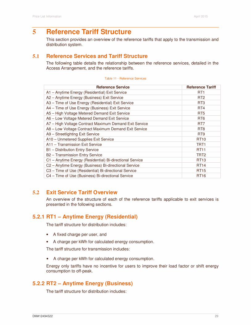
The following table details the relationship between the reference services, detailed in the Access Arrangement, and the reference tariffs.
Table 11 - Reference Services
Reference Service Reference Tariff
A1 – Anytime Energy (Residential) Exit Service RT1
A2 – Anytime Energy (Business) Exit Service RT2
A3 – Time of Use Energy (Residential) Exit Service RT3
A4 – Time of Use Energy (Business) Exit Service RT4
A5 – High Voltage Metered Demand Exit Service RT5
A6 – Low Voltage Metered Demand Exit Service RT6
A7 – High Voltage Contract Maximum Demand Exit Service RT7
A8 – Low Voltage Contract Maximum Demand Exit Service RT8
A9 – Streetlighting Exit Service RT9
A10 – Unmetered Supplies Exit Service RT10
A11 – Transmission Exit Service TRT1
B1 – Distribution Entry Service RT11
B2 – Transmission Entry Service TRT2
C1 – Anytime Energy (Residential) Bi-directional Service RT13
C2 – Anytime Energy (Business) Bi-directional Service RT14
C3 – Time of Use (Residential) Bi-directional Service RT15
C4 – Time of Use (Business) Bi-directional Service RT16
5.2 Exit Service Tariff Overview An overview of the structure of each of the reference tariffs applicable to exit services is presented in the following sections.
5.2.1 RT1 – Anytime Energy (Residential)
The tariff structure for distribution includes:
• A fixed charge per user, and
• A charge per kWh for calculated energy consumption.
The tariff structure for transmission includes:
• A charge per kWh for calculated energy consumption.
Energy only tariffs have no incentive for users to improve their load factor or shift energy consumption to off-peak.
5.2.2 RT2 – Anytime Energy (Business)
The tariff structure for distribution includes:
DM#12494522 29
Price List Information April 2015
• A fixed charge per user, and
• A charge per kWh for metered energy consumption.
The tariff structure for transmission includes:
• A charge per kWh for metered energy consumption.
Energy only tariffs have no incentive for users to improve their load factor or shift energy consumption to off-peak
5.2.3 RT3 – Time of Use Energy (Residential)
The tariff structure for distribution includes:
• A fixed charge per user;
• A charge per kWh for metered on peak energy consumption; and
• A charge per kWh for metered off peak energy consumption.
The tariff structure for transmission includes:
• A charge per kWh for metered on peak energy consumption; and
• A charge per kWh for metered off peak energy consumption.
Time of use tariffs have the incentive for users to manage their energy consumption to shift energy consumption from on-peak to off-peak.
5.2.4 RT4 – Time of Use Energy (Business)
The tariff structure for distribution includes:
• A fixed charge per user;
• A charge per kWh for metered on peak energy consumption; and
• A charge per kWh for metered off peak energy consumption.
The tariff structure for transmission includes:
• A charge per kWh for metered on peak energy consumption; and
• A charge per kWh for metered off peak energy consumption.
Time of use tariffs have the incentive for users to manage their energy consumption to shift energy consumption from on-peak to off-peak.
5.2.5 RT5 – High Voltage Metered Demand
The tariff structure is based on the metered demand of the user, with a discount to the demand charge based on the ratio of off peak energy to total energy used. In addition the tariff has a demand length tariff component for users with demand greater than 1,000 kVA. There is a separate metering charge that picks up the capital and operating costs for the metering asset.
This tariff has a mix of incentives for the user to manage their electricity consumption.
The demand used is a running 12-month peak. This provides a clear incentive to manage the peak demand because any excessive demand recorded in one month then impacts
DM#12494522 30
Price List Information April 2015
upon the demand charge for the next 12 months. The demand length charge is also based on the running 12-month peak.
The second incentive is the off peak energy discount which is based upon the ratio of off peak energy to total energy used. The maximum discount is 50% for off peak energy usage only and for an equal use of on and off peak energy the discount is 25%.
5.2.6 RT6 – Low Voltage Metered Demand
The tariff structure is identical to RT5 – High Voltage Metered Demand.
5.2.7 RT7 – High Voltage Contract Maximum Demand
The tariff structure requires the user to nominate a contracted maximum demand (CMD) that reasonably reflects their expected annual peak demand. In addition the tariff has a demand length tariff component also based on the CMD. There is a monthly penalty for any demand excursion above the CMD. All prices are in terms of $ per kVA.
The distribution component of the prices is zonal and there are 5 zones ranging from CBD to rural. This is because the costs of supply are seen to be dependent on the nature of the network that varies according to the location and consequent construction standard and cost.
There are also separate charges for administration and metering.
The transmission component of the tariff is nodal with prices based on the zone substation to which the user is connected.
This tariff has a mix of incentives for the user to manage their electricity consumption.
The demand is in kVA rather than kW so that there is a clear benefit from managing the power factor as close to unity as possible. For example, improving the power factor from 0.7 to 0.8 will reduce the demand charge by 12.5%.
The second incentive is to manage the peak demand, which can be achieved by improving the load factor and by containing the peak demand. This incentive is very strong and the user has flexibility in the options available for managing the demand. The penalty for exceeding the contract maximum demand provides additional incentive.
The demand length charge provides an incentive for the user to locate as close as possible to the zone substation. For existing users there is no real opportunity to respond to this incentive, but for new users there is some ability to respond.
The transmission component of the price is nodal so that there is a clear signal for users to locate near to the lower price substations. This may or may not be achievable depending on the individual user circumstances.
5.2.8 RT8 – Low Voltage Contract Maximum Demand
The tariff structure is identical to RT7 – High Voltage Contract Maximum Demand with the addition of a low voltage charge that reflects the additional cost for usage of the low voltage distribution network.
DM#12494522 31

Price List Information April 2015
5.2.9 RT9 – Streetlighting
Streetlights do not have metering information to support either the initial setting of the tariff or the billing of users based on energy consumption or energy demand and therefore the energy consumption must be estimated based on burn hours and globe wattage.
The tariff structure for distribution includes:
• A fixed charge per user; and
• A charge per kWh for calculated energy consumption.
The tariff structure for transmission includes:
• A charge per kWh for calculated energy consumption.
In addition there is a charge to reflect the capital and operating costs of the streetlight asset itself. Western Power owns the assets and the revenue is included within the reference service revenue. The tariff structure for the streetlight asset is simply a fixed charge per light based on the type and rating of the light.
5.2.10 RT10 – Unmetered Supplies
Unmetered supplies do not have metering information to support either the initial setting of the tariff or the billing of users based on energy consumption or energy demand. However there is a requirement for the user to provide sufficient load data so that the energy consumption can be calculated. As such the available information is user connection and energy consumption.
The tariff structure for distribution includes:
• A fixed charge per user; and
• A charge per kWh for calculated energy consumption.
The tariff structure for transmission includes:
• A charge per kWh for calculated energy consumption.
5.2.11 TRT1 – Transmission
The tariff is based on the zone substation to which the user is connected. The user will pay the use of system, common service and control system service charges. There is also a separate metering charge. All prices are in $ per kW.
The tariff structure requires the user to nominate a CMD, in kWs, that reasonably reflects their expected annual peak demand. There is a monthly penalty for any demand excursion above the CMD.
The incentive is clearly for the user to manage their peak demand through the initial nomination of the CMD and also the monthly penalty for exceeding the CMD.
5.3 Entry Service Tariff Overview
An overview of the structure of each of the reference tariffs applicable to entry services is presented in the following sections.
DM#12494522 32
Price List Information April 2015
5.3.1 RT11 – Distribution
The transmission charge is identical to the charge for a transmission connected generator in that the generator nominates a declared sent out capacity (DSOC) and the charge is based on the transmission nodal price at the nearest transmission entry point. The transmission charge for use of system is in $ per kW. Unlike the transmission exit reference tariff (TRT1) there is no common service charge. The generator must also pay the connection charge which is also expressed in terms of $ per kW.
The generator’s DSOC is in kW and is corrected for losses from the zone substation to the generator site, for purposes of calculation of the transmission price component.
The distribution charge is based on the zonal CMD demand length price. There is no demand only charge. As such the distribution charge for generators with demand less than 1,000 kVA is zero. There is also a separate metering charge.
The DSOC must be nominated in kW for the transmission charge and in kVA for the distribution charge. However the power factor is assumed to be unity for the purpose of charging because the power factor will not generally be within the control of the generator.
The incentive for distribution-connected generators is to locate as near as possible to the zone substation although for generators with a DSOC less than 1,000 kVA there is no such incentive. However, small generators are not considered to require strong locational incentives because the network will generally not be impacted to any significant extent.
The transmission component also contains a locational signal. Like for TRT2 customers, there is a monthly penalty for any demand excursion above the DSOC that has not been authorised by System Management.
5.3.2 TRT2 – Transmission
The tariff is based on the zone substation to which the generator is connected. The generator will pay the entry point use of system and control system service charges. There is also a separate metering charge. All prices are in $ per kW.
The tariff structure requires the generator to nominate a DSOC, in kWs, that reflects their maximum intended export capacity. There is a monthly penalty for any demand excursion above the DSOC that has not been authorised by System Management.
5.4 Bi-directional Service Tariff Overview
An overview of the structure of each of the reference tariffs applicable to bi-directional services is presented in the following sections. For all four bi-directional services, the tariffs are equivalent to the reference service upon which it is based.
5.4.1 RT13 – RT16
The tariff structure of these tariffs is based on the structures of tariffs RT1-4 detailed in sections 5.2.1 to 5.2.4.
DM#12494522 33

Price List Information April 2015
6 Derivation of Transmission System Tariff Components This section describes the methodology used to calculate transmission reference tariff components.
6.1 Cost Reflective Network Pricing
6.1.1 General
The Cost Reflective Network Pricing (CRNP) cost allocation method allocates the revenue requirement to all network elements, based on their Gross Optimised Deprival Value (GODV), then determines the use made of each network element by each connection point during the survey period.
The CRNP cost allocation process requires detailed network analysis and involves the following steps:
1. determining the annual revenue requirement for individual transmission shared network assets (see below);
2. determining the network load and generation pattern;
3. performing a load-flow to calculate the MVA loading on network elements;
4. determining the allocation of generation to loads;
5. determining the utilisation of each asset on the network by each connection point;
6. allocating the revenue requirement of individual network elements to each user based on the assessed usage share; and
7. determining the total cost allocated to each connection point by adding the share of the costs of each individual network element attributed to each point in the network.
6.1.2 Allocation of Generation to Load
A major assumption in the use of the CRNP methodology is the allocation of generation to load using the ‘electrical distance’. With this approach, a greater proportion of load at a particular location is supplied by generators that are electrically closer than those that are electrically remote. The electrical distance is the impedance between the two locations, and this can readily be determined through a standard ‘fault level calculation’. Once the assumption has been made as to the proportion that each generator actually supplies each load for a particular load and generation condition (time of day) it is possible to trace the flow through the network that results from supplying each load (or generator).
The utilisation that any load makes of any element is then simply the ratio of the flow on the element resulting from the supply to this load to the total flow on the element made by all loads and generators in the system.
DM#12494522 34

Price List Information April 2015
6.1.3 Operating Conditions for Cost Allocation
The choice of operating conditions is important in developing prices using the CRNP methodology. The use made of the network by particular loads and generators will vary depending on the load and generation conditions on the network at the time. The National Electricity Rules (NER) sets out the principles to apply in determining the sample of operating conditions considered.
The load and generation patterns used to establish transmission prices should include all operating scenarios that result in most stress in the network and for which network investment may be contemplated. The operating conditions chosen should broadly correspond to the times at which high demands drive network expansion decisions. Operating conditions should be included that impose peak loading conditions on particular elements, recognising that these may occur at times other than for peak demand.
Consistent with these principles, the operating conditions to be used for the cost allocation process for the transmission system as are as follows:
• Load and generation conditions shall be actual operating conditions from the previous 12 months; and
• Operating conditions shall include data for every node for every half hour where system peak demand is greater than an amount such that data from 10 individual summer days and 10 individual winter days are included.
6.2 Price Setting for Transmission Reference Services
Transmission tariffs for exit and entry services are fixed and are generally expressed as $/kw/annum. Generally, transmission prices are derived by dividing the cost pool, either in its entirety or at a zone substation level, by the assigned maximum demand applying to those assets. However, the details of some parts of the process are complex and explained in more detail in the following sections.
6.2.1 Transmission Pricing Model
Once Transmission assets are valued and T-price (see below for details) has established the relativity of UOS prices the Transmission Pricing Model is used:
1. to calculate the annual revenue requirements for all respective cost pools (based on valuation data and the rate of return required); and
2. to scale the raw T-price UOS prices to give the required Use Of System cost pool revenues.
6.2.2 Connection Price
The Connection Price is a price for the utilisation of Western Power owned connection assets. The Connection Price reflects the total annual costs allocated to the connection assets divided by the total usage at all points. The Connection Price is calculated by taking the Connection Cost Pool Revenue and dividing it by the aggregate of relevant CMDs and DSOCs (over all Exit or Entry points where the charge is applied).
DM#12494522 35
Price List Information April 2015
Connection charges for connection points on the distribution system will be differentiated between loads and generators by applying the principles applied to the transmission shared system4. This results in generators paying approximately a quarter of the price as for loads.
Connection charges for connection points on the transmission system are not published but are determined subject to the specific connection arrangements. These connection charges are individually calculated to reflect the actual connection assets that apply to that user. The amount of the charge is based on achieving a regulated return on all relevant assets and an allocation of the transmission network operating costs.
6.2.3 Use of System (UOS) Prices
Consistent with the NER, the proportion of the transmission reference service revenue that is allocated to Transmission UOS is allocated to each and every connection point using a CRNP method. CRNP assigns a proportion of shared network costs to individual user connection points.
6.2.3.1. T-Price
Western Power uses T-price to establish the relativity of UOS prices for each exit and entry point. T-price is a modelling tool to allocate network costs using CRNP. T-price requires significant work to establish all of the inputs and to run the model. However, in summary:
• The GODV of every branch and node of the network is allocated. Every node is classified as either Exit or Entry, and every Branch is classified as either shared or dedicated to consumers or dedicated to generators.
• Electrical configuration and parameters of the network are established (PSSE system Raw Data file).
• Interval demand data is assembled for all entry and exit points.
• Load flow analysis is carried out so that all network element costs are allocated to each zone substation based on usage of those network elements.
• The costs for all entry and exit points are then converted to prices by assigning a maximum demand to each node and using that demand to calculate a price in terms of $/kW/annum.
6.2.3.2. UOS Price Moderation
The application of CRNP for UOS prices can introduce volatility to individual prices as a result of changes in network usage beyond the control of any one user. It is hence appropriate to moderate any price fluctuations to mitigate price shock and improve certainty to customers. Annual variations to TUOS prices are therefore scaled and moderated as follows:
• annual changes to be constrained within a bandwidth of ± 5%; and
• the mid-point of the band set to recover the required cost pool revenue.
4 By adopting the principle of 20 per cent of costs being allocated to generation and the remaining 80
per cent to loads.
DM#12494522 36

Price List Information April 2015
6.2.3.3. UOS Prices – Exit Points
UOS prices for Exit Points are calculated within the constraints of the UOS Price Moderation specified above to recover the UOS for Loads Cost Pool Revenue.
6.2.3.4. UOS Prices – Entry Points
UOS prices for Entry Points are calculated within the constraints of the UOS Price Moderation specified above to recover the UOS for Generators Cost Pool Revenue.
6.2.4 Common Service Price for Loads
The Common Service Price is expressed in c/kW/day and is uniform for all exit points. The Common Service Price is calculated by taking the Common Service Cost Pool Revenue and dividing it by the aggregate of relevant CMDs (over all Exit points where the charge is applied).
6.2.5 Control System Service Price
The Control System Service Price is expressed in c/kW/day. Separate Prices for consumers and generators are calculated based on the respective cost pools but are uniform for each.
6.2.5.1. Control System Service for Loads
The Control System Services price for Loads is calculated by taking the Control System Services for Loads Cost Pool Revenue and dividing it by the aggregate of relevant CMDs (over all Exit points where the charge is applied).
6.2.5.2. Control System Service for Generators
The Control System Services price for Generators is calculated by taking the Control System Services for Generators Cost Pool Revenue and dividing it by the aggregate of relevant DSOCs (over all Entry Points where the charge is applied).
6.2.6 Transmission Tariff Setting
The following table details the forecast transmission revenue which will be collected from transmission connection points and the total amount that will be collected from distribution connection points (please see section 6.3 for further details).
Table 12 - Transmission Revenue Forecast for 2015/16 ($M Nominal)
Forecast Total MW
Number Customers
Forecast Transmission
Revenue Recovered
Transmission Exit 728 28 35.3
Transmission Entry 5948 30 51.7
Distribution Users 3685 1,316,872 238.6
Transmission Standby 3.3
Total Revenue Cap Revenue 328.8
DM#12494522 37

Price List Information April 2015
6.3 Price Setting for Distribution Reference Services
The tariffs for connection points on the transmission system do not collect the full transmission reference service revenue entitlement. Connection points on the distribution system utilise the transmission system as well as the distribution system. The remainder of the transmission reference service revenue entitlement is collected from tariffs for connection points on the distribution system.
Charges are determined for each direct connected transmission user based on respective CMDs. The revenues from these users are then deducted from the revenue entitlement for that substation to give a net revenue amount to be recovered from users connected to that substation via tariffs for connection points on the distribution system.
Reference tariffs for users connected to the distribution system with a peak demand >1 MVA incorporate transmission nodal prices. The transmission pass-through revenue, net of the revenues from the >1 MVA users, is then allocated in aggregate to the various small customer groupings on the basis of loss adjusted any time maximum demand (ATMD) for each grouping (further described below).
A number of processes take place to determine transmission prices that match the structure of distribution reference tariffs so that a full suite of bundled tariffs can be produced.
Transmission prices take a range of forms, as discussed in section 5. The CMD tariffs are based on a nominated peak demand in terms of kVA. The CMD tariffs are nodal in that they are based on the transmission node to which the load user is connected. All other tariffs are uniform across the Western Power Network.
DM#12494522 38
Price List Information April 2015
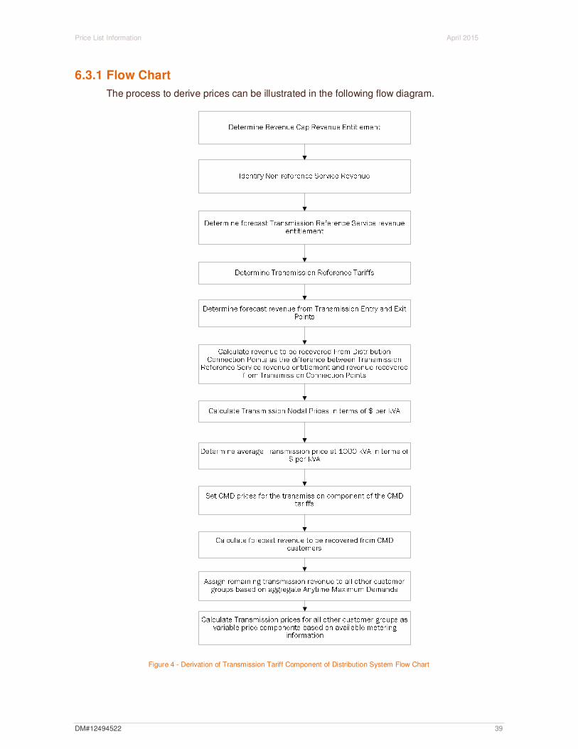
6.3.1 Flow Chart
The process to derive prices can be illustrated in the following flow diagram.
Figure 4 - Derivation of Transmission Tariff Component of Distribution System Flow Chart
DM#12494522 39

Price List Information April 2015
Each step in this process to derive transmission component of the distribution system reference tariffs is described in more detail as follows. The first two steps of determining the revenue entitlement and prices for transmission connected users have been covered earlier.
6.3.2 Calculate the Forecast Revenue to be recovered from Distribution-Connected Users
It is assumed at this stage that the forecast transmission revenue entitlement has been determined and transmission reference tariffs set. By applying the reference tariffs to the forecast transmission-connected user data, the revenue to be recovered from transmission entry and exit points can be forecast. The residual is the revenue that must be recovered from connection points on the distribution system.
6.3.3 Calculate Transmission Nodal Prices in terms of $ per kVA
To calculated the transmission prices in terms of $ per kVA the zone substation power factors must be determined. The power factors are measured at the low voltage bus of the zone substations at system peak. To create a single nodal price the transmission use of system, common service and connection prices are added together for each zone substation. Multiplying that price by the power factor then provides the price in terms of $/kVA.
There is an additional factor taken into account at this stage. The Urban and CBD prices are set to be uniform for distribution-connected users. To achieve this, a weighted average transmission nodal price and a weighted average power factor are used.
This step is taken for a number of reasons. It does not make sense for users across the Perth metropolitan area to see a range of prices depending on location. For example users can be connected to one zone substation for a period of time and then transferred to a different zone substation for operational reasons. Individual zone substation nodal prices would result in such a user seeing a price change although they had not changed anything from their perspective. From an administrative perspective it would be very difficult to manage such a situation. Price changes would also need to be managed within any side constraints imposed on price movements.
Another reason for this approach is that nodal prices are designed to give users an economic signal in terms of location. However, in an urban environment it is difficult for users to respond to any economic signal because land zoning and availability will normally be the determining factor in location rather than cost of supply.
This process produces a set of zone substation prices that are individual for Rural, Mixed and Mining substations and uniform for the CBD and Urban substations. These transmission nodal prices apply to connection points on the distribution system with demands equal to or greater than 7,000 kVA. This principle is established because the cost that a 7,000 kVA user imposes on the transmission network will be the same whether connected to the distribution or transmission networks.
For users with CMD below 7,000 kVA the factor of load diversity becomes more relevant. In addition, the price must be structured to fit into the bundled tariff structure for all CMD users with demands greater than 1,000 kVA.
DM#12494522 40

Price List Information April 2015
6.3.4 Determine Average Transmission Price at 1,000 kVA
At this stage we have the transmission nodal prices at 7,000 kVA. We also have established that the transmission price in terms of $/kVA at 1,000 kVA will be uniform for all users and will be the same from 0 to 1,000 kVA. The task is to establish that uniform price.
Transmission costs are allocated to all users on the basis of anytime peak kVA demand. The transmission price is simply the revenue to be recovered from users with demands below 1,000 kVA divided by the sum of the anytime maximum demands of all those users.
The anytime maximum demands are not metered for the vast majority of users with demands below 1,000 kVA. The energy consumption is metered and the anytime maximum demands are estimated by applying load factors based on Industry Codes. The industry codes and associated load factors were developed using sample data for actual representative user types.
At this stage the size of the revenue pool is not established. The revenue pool will be the amount defined by the following formula:
RPBelow 1,000 = RP Total – RP Over 7,000 - RP 1,000 to 7,000
where,
RPBelow 1,000 = revenue to be recovered from users with demands below 1,000 kVA
RP Total = revenue to be recovered from all distribution connected users
RP Over 7,000 = revenue to be recovered from users with demands greater than 7,000 kVA
RP 1,000 to 7,000 = revenue to be recovered from users with demands between 1,000 and 7,000 kVA
This equation has unknowns in several terms at this stage. The revenue to be recovered from users with demands greater than 7,000 kVA is known because it is equal to the forecast demands of those users multiplied by the nodal price for each user.
The next step is to determine the pricing structure for users with demands between 1,000 and 7,000 kVA. To facilitate the bundling of transmission and distribution components in reference tariffs for connection points on the distribution system the transmission price structure must be consistent with the distribution price structure. For these users this means the prices will be in “rate block” structure and take the form:
User Charge 1,000 to 7,000 = (Price At 1,000 * 1,000 kVA) + (Price 1,000 to 7,000 *(CMD User – 1,000 kVA))
Where:
User Charge 1,000 to 7,000 = the use of system charge for a user with CMD between 1,000 and 7,000 kVA
Price At 1,000 = the average use of system price for all users with CMD below 1,000 kVA
DM#12494522 41

Price List Information April 2015
Price 1,000 to 7,000 = the use of system for this user with CMD between 1,000 and 7,000 kVA
CMD User = the contract maximum demand for that user
The Price 1,000 to 7,000 will be different for each zone substation but can be calculated by the formula:
Price 1,000 to 7,000 = [(Price At 7,000 * 7,000 kVA) - (Price At 1,000 * 1,000 kVA)]/6,000 kVA
So we now have a formula to calculate the price for each user with CMD between 1,000 and 7,000 kVA with the unknown being the price at 1,000 kVA. We now have a single unknown (Price At 1,000) that can now be solved in the above equation which now must be expanded as below.
Original Equation:
RP Below 1,000 = RP Total – RP Over 7,000 - RP 1,000 to 7,000
Expansion of each term:
RP Below 1,000 = ∑ User anytime maximum demands multiplied by Price At 1,000
RP Total = Total transmission revenue entitlement allocated to distribution-connected users
RP Over 7,000 = ∑ Individual demands for users greater than 7,000 kVA anytime maximum demands multiplied by the nodal price at the zone substation to which the user is connected
RP 1,000 to 7,000 = ∑ User charges for all users with CMDs between 1,000 and 7,000 kVA
At this stage of the process we have the average price at and below 1,000 kVA, the nodal price for each zone substation for demands between 1,000 and 7,000 kVA and the nodal price for demands greater than 1,000 kVA. This has set the transmission tariffs for CMD users.
The rate blocks were developed using the principle of a straight-line transition from the charge at 1,000 kVA to the charge at 7,000 kVA. When converted back to prices the actual prices at any demand can be mapped and in fact the transition from a flat price below 1,000 kVA to a flat price above 7,000 kVA is a 1/x curve. The following graph illustrates the price outcomes for the above process. A number of substations have been chosen to represent the range of prices across urban and rural substations
DM#12494522 42
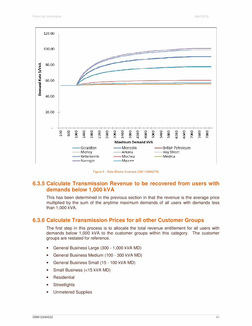
Price List Information April 2015
Figure 5 - Rate Blocks Example (DM 12894279)
6.3.5 Calculate Transmission Revenue to be recovered from users with demands below 1,000 kVA
This has been determined in the previous section in that the revenue is the average price multiplied by the sum of the anytime maximum demands of all users with demands less than 1,000 kVA.
6.3.6 Calculate Transmission Prices for all other Customer Groups
The first step in this process is to allocate the total revenue entitlement for all users with demands below 1,000 kVA to the customer groups within this category. The customer groups are restated for reference.
• General Business Large (300 - 1,000 kVA MD)
• General Business Medium (100 - 300 kVA MD)
• General Business Small (15 - 100 kVA MD)
• Small Business (<15 kVA MD)
• Residential
• Streetlights
• Unmetered Supplies
DM#12494522 43

Price List Information April 2015
The result of this process is an amount of revenue that must be recovered within each customer group. At this stage the customer group users are mapped to reference tariff groups together with their associated revenues. We then have revenue entitlements assigned to reference tariffs. The process then becomes one of matching the revenue entitlement to metered information to produce tariff components.
In the case of Transmission reference tariff components the cost pools are allocated on the basis of demand. The tariffs now being considered do not have metered values for demand and on that basis; energy is used as a proxy for demand. The revenue is recovered entirely through the variable component of the tariffs, which in each of these tariffs is the energy rate. Thus the tariff components are in terms of cents per kWh.
In the case of unmetered supplies, streetlights, energy small and energy large tariffs the price is calculated by the simple formula:
Price Tariff = Forecast Revenue Entitlement for Tariff /Total Forecast Energy for Tariff
In the case of the time of use energy tariffs the transmission revenue allocated to those tariffs is recovered through both the on-peak and off-peak energy amounts. It is essentially the on-peak demand and therefore on-peak energy that drives the cost of the transmission network. However off-peak energy must also be served and a proportion of the revenue is recovered through the off-peak energy.
In fact approximately 30% of the forecast revenue entitlement is recovered through the off-peak energy and 70% through the on-peak energy. This ratio is chosen to achieve three outcomes:
• It clearly recovers most of the cost from on-peak usage which is the main driver of transmission costs;
• It allows for some of the costs to be recovered from off-peak energy usage to provide for equity between users with different load patterns; and
• It provides a clear economic signal to encourage off-peak energy usage that has the benefit of reducing network costs resulting in lower reference tariffs for all users.
DM#12494522 44

Price List Information April 2015
6.3.7 Transmission Components of Distribution Reference Tariffs Forecast Revenue
The following table details the forecast transmission reference service revenue, by tariff, which will be collected from distribution connection points.
Table 13 - Transmission Reference Service Revenue Recovered from Distribution Connection Points for 2015/16 ($M Nominal)
kWh ATMD kVA Number
Customers
Forecast Transmission
Revenue Recovered
RT1 - Anytime Energy (Residential) 5,040,980,245 1,970,869 927,656 84.4
RT2 - Anytime Energy (Business) 1,180,341,029 535,936 85,671 23.5
RT3 - Time of Use Energy (Residential) 159,278,898 63,877 21,594 2.6
RT4 - Time of Use Energy (Business) 1,963,747,971 1,168,543 14,951 38.2
RT5 - High Voltage Metered Demand 363,429,118 111,092 132 5.1
RT6 - Low Voltage Metered Demand 1,642,782,344 486,759 2,479 25.4
RT7 - High Voltage Contract Maximum
Demand 3,066,884,986 850,058 285 51.9
RT8 - Low Voltage Contract Maximum
Demand 223,356,447 73,246 61 4.0
RT9 – Streetlighting 123,353,806 30,149 248,492 1.3
RT10 - Unmetered Supplies 32,680,258 5,095 15,531 0.2
RT11 - Distribution Entry 0 0 20 1.3
RT13 – Anytime Energy (Residential) Bi
directional
0 0 0 0
RT14 – Anytime Energy (Business) Bi
directional
0 0 0 0
RT15 – Time of Use (Residential) Bi
directional
0 0 0 0
RT16 – Time of Use (Business) Bi
directional
0 0 0 0
TOTAL - Reference Service 13,796,835,102 5,295,623 1,316,872 237.9
TOTAL – Non-Reference Service 0.7
TOTAL 238.6
6.4 Annual Price Review
As described in the Access Arrangement, revenue cap service revenue is reviewed annually and adjusted if necessary for under or over recovery. Together with changes to user CMDs and DSOCs (including zone substation maximum demands) it is consequently necessary to adjust prices annually also.
DM#12494522 45

Price List Information April 2015
7 Derivation of Distribution System Tariff Components This section describes the methodology used to calculate distribution reference tariff components.
The cost allocation process reflects the costs of supply for a customer group reasonably accurately. The process for determining prices for that customer group, while ideally similar in principle, is somewhat different in that it needs to take into account other factors such as equity, simplicity and efficiency (e.g. existing metering type).
Prices are determined with pre loss-adjusted ATMDs.
The Code requires uniform reference tariffs for all users with annual energy demand below 1 MVA, which equates to approximately all but 500 connected to the Western Power Network. Users with energy demand below 1 MVA will exhibit the full range of energy consumption patterns. It is therefore clear that any tariff structure will not be totally cost reflective. However, the assumptions that are made in allocating users to particular load groups and in deriving the cost of supply to those customer groups, and the consequent prices, are all considered reasonable. Through the process described in this paper the tariff settings are derived through as rigorous a process as is possible taking into account the information available and the requirements of the Code.
The distribution reference tariff components include the costs associated with the Tariff Equalisation Contribution (TEC). Section 7.12 of the Code sets out the requirement for Western Power to recover TEC through distribution reference tariffs for exit services (Western Power has extended this to include bi-directional services to be consistent with the Code Objective). Section 7.6 details the amounts associated with TEC that are embedded within the distribution reference tariff components.
7.1 Price Setting
This section details the methodology used to derive the tariff components from the cost pools, customer groups and locational zones.
7.1.1 Tariff Components
Distribution reference tariffs have been developed to enable users with different loads and usage patterns to choose the most appropriate form for them. The tariffs have fixed and variable components and are generally compatible with existing forms of user metering.
The components of each reference tariff are shown in the following table.
DM#12494522 46
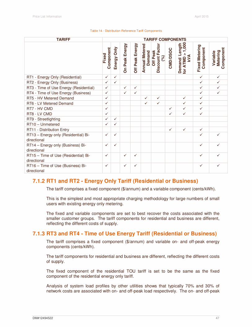
Price List Information April 2015
Table 14 - Distribution Reference Tariff Components
TARIFF TARIFF COMPONENTS
Fix
ed
Co
mp
on
en
t
En
erg
y O
nly
On
Pe
ak E
ne
rgy
Off
Pe
ak E
ne
rgy
An
nu
al
Mete
red
Dem
an
d
Off
Pea
kD
isco
un
t F
acto
r(%
)
CM
D/D
SO
C
De
man
d/
Le
ng
thfo
r A
TM
D >
1,0
00
kV
A
Fix
ed
Me
teri
ng
Co
mp
on
en
t
Vari
ab
leM
ete
rin
gC
om
po
ne
nt
RT1 - Energy Only (Residential) � � � �
RT2 - Energy Only (Business) � � � �
RT3 - Time of Use Energy (Residential) � � � � �
RT4 - Time of Use Energy (Business) � � � � �
RT5 - HV Metered Demand � � � � �
RT6 - LV Metered Demand � � � � �
RT7 - HV CMD � � � �
RT8 - LV CMD � � � �
RT9 - Streetlighting � �
RT10 – Unmetered � �
RT11 - Distribution Entry � � �
RT13 – Energy only (Residential) Bi
directional
� � � �
RT14 – Energy only (Business) Bi
directional
� � � �
RT15 – Time of Use (Residential) Bi
directional
� � � � �
RT16 – Time of Use (Business) Bi
directional
� � � � �
7.1.2 RT1 and RT2 - Energy Only Tariff (Residential or Business)
The tariff comprises a fixed component ($/annum) and a variable component (cents/kWh).
This is the simplest and most appropriate charging methodology for large numbers of small users with existing energy only metering.
The fixed and variable components are set to best recover the costs associated with the smaller customer groups. The tariff components for residential and business are different, reflecting the different costs of supply.
7.1.3 RT3 and RT4 - Time of Use Energy Tariff (Residential or Business)
The tariff comprises a fixed component ($/annum) and variable on- and off-peak energy components (cents/kWh).
The tariff components for residential and business are different, reflecting the different costs of supply.
The fixed component of the residential TOU tariff is set to be the same as the fixed component of the residential energy only tariff.
Analysis of system load profiles by other utilities shows that typically 70% and 30% of network costs are associated with on- and off-peak load respectively. The on- and off-peak
DM#12494522 47
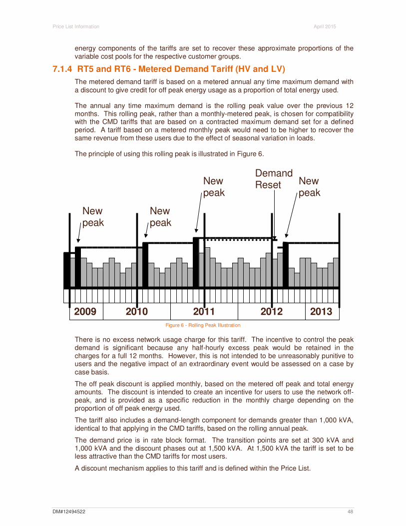
Price List Information April 2015
energy components of the tariffs are set to recover these approximate proportions of the variable cost pools for the respective customer groups.
7.1.4 RT5 and RT6 - Metered Demand Tariff (HV and LV)
The metered demand tariff is based on a metered annual any time maximum demand with a discount to give credit for off peak energy usage as a proportion of total energy used.
The annual any time maximum demand is the rolling peak value over the previous 12 months. This rolling peak, rather than a monthly-metered peak, is chosen for compatibility with the CMD tariffs that are based on a contracted maximum demand set for a defined period. A tariff based on a metered monthly peak would need to be higher to recover the same revenue from these users due to the effect of seasonal variation in loads.
The principle of using this rolling peak is illustrated in Figure 6.
Demand New New Reset
New peak
New peak
peak peak
2009 2010 2011 2012 2013 Figure 6 - Rolling Peak Illustration
There is no excess network usage charge for this tariff. The incentive to control the peak demand is significant because any half-hourly excess peak would be retained in the charges for a full 12 months. However, this is not intended to be unreasonably punitive to users and the negative impact of an extraordinary event would be assessed on a case by case basis.
The off peak discount is applied monthly, based on the metered off peak and total energy amounts. The discount is intended to create an incentive for users to use the network off-peak, and is provided as a specific reduction in the monthly charge depending on the proportion of off peak energy used.
The tariff also includes a demand-length component for demands greater than 1,000 kVA, identical to that applying in the CMD tariffs, based on the rolling annual peak.
The demand price is in rate block format. The transition points are set at 300 kVA and 1,000 kVA and the discount phases out at 1,500 kVA. At 1,500 kVA the tariff is set to be less attractive than the CMD tariffs for most users.
A discount mechanism applies to this tariff and is defined within the Price List.
DM#12494522 48

Price List Information April 2015
7.1.5 RT7 and RT8 - Contract Maximum Demand Tariff (HV and LV)
The HV component of the CMD tariff is set to reflect a price that results in a user charge that is greater than the user incremental cost of supply but less than the stand-alone cost of supply. To achieve this outcome the two costs of service are modelled for each of the HV and LV CMD users.
Customers on transition tariffs are modelled, for pricing setting purposes, as contract maximum demand tariff customers.
The price structure is based on two particular components. There is a component that is directly linked to the nominated maximum demand which is in terms of $/kVA. The second component is based on a combination of the maximum demand and the length of HV feeder from the zone substation to the user’s connection point. This price component is expressed in terms of $/kVA.km. Both of these tariff components are set to be uniform at 1,000 kVA and to be fully cost reflective at 7,000 kVA. This structure is consistent with the transmission CMD tariff for distribution connected customers.
The “demand/length” component of the tariff cannot be used in isolation because it distorts the charge for users either very close to the zone substation, where the cost could be virtually zero, or at a long distance from the substation, where the charge could be unreasonably high. The “demand” component of the tariff ameliorates this distortion because it recognises that the cost of supply of a user does not only relate to the distance from the zone substation but also relates to the demand that the user places on the network.
The effect of the pricing structure is that, for a fixed demand, the charge to a user increases as distance to the zone substation increases. This is effectively providing a fixed and variable component to the price for identical users depending on their distance from a zone substation. In a similar manner users at the same distance from a zone substation will pay more as their demand increases.
An additional feature of this price structure is that the price is not linear in relation to the demand.
For the demand only component, the price at 1,000 kVA is uniform for each of the locational zones and is reflective of the average HV cost of the network per KVA demand. However, as the demand increases, the price declines recognising that the cost of supply declines on a per unit basis, as the demand increases.
The demand/length component is set to zero at 1,000 kVA. This is consistent with the requirement that all tariffs are uniform below 1,000 kVA demand. The price above 7,000 kVA is uniform and the price varies continuously between 1,000 and 7,000 kVA.
In setting the CMD tariffs both components are adjusted so that for each of the users with demands greater than 1,000 kVA, their charge will fall between the incremental and standalone cost. The process to derive the settings is described as follows.
Demand Component of the CMD Tariff
The price at 7,000 kVA is individually set for each zone. The price is adjusted to provide a best fit so that users will see a charge that is between the incremental and stand-alone cost. This is done in combination with the demand/length component setting. However it is clear that the price at 7,000 kVA should reflect the actual costs of the networks that supply
DM#12494522 49
Price List Information April 2015
these users. As such the cost for the CBD zone will be the highest, the Urban zone the next highest and so on so that the rural zone is the cheapest.
At this stage we have the distribution nodal prices at 7,000 kVA. We also have established that the distribution price in terms of $/kVA at 1,000 kVA will be uniform for all users and will be the same from 0 to 1,000 kVA. The task is to establish that uniform price. At 1,000 kVA the demand/length price is zero so the demand price should reflect the average network price for all users in terms of $/kVA.
Distribution costs are allocated to all users on the basis of anytime peak kVA demand adjusted for losses. The distribution price is simply the revenue to be recovered from users with demands below 1,000 kVA divided by the sum of the anytime maximum demands of all those users.
The anytime maximum demands are not metered for the vast majority of users with demands below 1,000 kVA. The energy consumption is metered and the anytime maximum demands are estimated by applying load factors based on “Industry Codes”. The industry codes and associated load factors were developed using sample data for actual representative user types.
At this stage the size of the revenue pool for users with demands below 1,000 kVA is not established. The revenue pool will be the amount defined by the following formula:
RP Below 1,000 = RP Total – RP Over 7,000 - RP 1,000 to 7,000
where:
RP Below 1,000 = revenue to be recovered from users with demands below 1,000 kVA
RP Total = revenue to be recovered from all distribution users
RP Over 7,000 = revenue to be recovered from users with demands greater than 7,000 kVA
RP 1,000 to 7,000 = revenue to be recovered from users with demands between 1,000 and 7,000 kVA
This equation has unknowns in each of the terms at this stage. The revenue pools will only be determined when the CMD tariff settings are established and the prices can be applied to the forecast user data for users with demands greater than 1,000 kVA. The price at 7,000 kVA is set by graphically plotting the charge outcomes for each of the users with demands above 7,000 kVA, in the locational zones, and setting a price that puts the charge outcomes between the incremental and stand-alone cost of supply. Graphs demonstrating this are included in section 7.2.
To facilitate the solving of the remaining terms of this equation the pricing settings for users with demands between 1,000 and 7,000 kVA must be determined. The tariffs are defined in terms of “rate block” structure and, for the demand component of the tariff, take the form:
User Demand Charge 1,000 to 7,000 = (Price At 1,000 * 1,000 kVA) + (Price 1,000 to 7,000
*(CMD User – 1,000 kVA))
where:
DM#12494522 50
Price List Information April 2015
User Demand Charge 1,000 to 7,000 = the demand charge for a user with CMD between 1,000 and 7,000 kVA
Price At 1,000 = the average demand price for all users with CMD below 1,000 kVA
Price 1,000 to 7,000 = the incremental demand price for this user with CMD between 1,000 and 7,000 kVA
CMD User = the contract maximum demand for that user
The Price 1,000 to 7,000 will be different for each locational zone but can be calculated by the formula:
Price 1,000 to 7,000 = [(Price At 7,000 * 7,000 kVA) - (Price At 1,000 * 1,000 kVA)]/6,000 kVA
So we now have a formula to calculate the price for each user with CMD between 1,000 and 7,000 kVA with the unknown being the price at 1,000 kVA. The price at 7,000 kVA has been previously set.
We now have a single unknown (Price At 1,000) that can now be solved in the above equation which now must be expanded as below.
Original Equation:
RP Below 1,000 = RP Total – RP Over 7,000 - RP 1,000 to 7,000
Expansion of each term:
RP Below 1,000 = ∑ User anytime maximum demands multiplied by Price At 1,000
RP Total = Total HV network revenue entitlement
RP Over 7,000 = ∑ Individual demands for users greater than 7,000 kVA anytime maximum demands multiplied by the zonal price at the zone substation to which the user is connected
RP 1,000 to 7,000 = ∑ User charges for all users with CMDs between 1,000 and 7,000 kVA
At this stage of the process we have the average price at and below 1,000 kVA, the demand price formula for each locational zone for demands between 1,000 and 7,000 kVA and the zonal price for demands greater than 7,000 kVA. This has set the demand component of the CMD tariffs.
Demand/Length Component of the CMD Tariff
The demand/length component of the tariff is set at zero at 1,000 kVA. It is also uniform at and above 7,000 kVA. The tariff is also designed to be expressed in “rate block” format so that the price is in terms of an incremental price above 1,000 kVA and up to 7,000 kVA and a uniform price above 7,000 kVA.
The price between 1,000 and 7,000 kVA is expressed as:
Price 1,000 to 7,000 = [(Price At 7,000 * 7,000 kVA) - (Price At 1,000 * 1,000 kVA)]/6,000 kVA
DM#12494522 51
Price List Information April 2015
The price settings are established in the same process as setting the demand settings in that the incremental and stand-alone costs are graphically plotted for every CMD user within each zone and the price settings are adjusted so that the user charges fit between the limits. Graphs demonstrating this are included in section 7.2.
At this stage, the price settings are established for both the demand and demand/length price components of the CMD tariffs. The forecast HV network revenue for the HV and LV CMD users can be calculated by applying the prices to the forecast user data and summing the charges for all users.
The prices for both the demand and demand/length components of the prices are illustrated in Figure 12.
7.1.6 Metering
The ideal way to price metering is to have a separate charge for the particular type of meter for each user. While this approach is technically feasible, it is extremely complex due to the technical and commercial variations in metering arrangements.
The alternative and more efficient approach is to use a standard metering charge in conjunction with each reference tariff to reflect the average cost of metering deployed to support application of the tariff.
However, the variation in metering costs for users within each tariff group can be marked and an average metering charge would disadvantage all smaller users. For example:
• residential users may be either single or three phase; and
• small business users with energy only or TOU energy metering may have meters director CT-connected.
Therefore, it is appropriate for small users to have a charge that varies with usage and therefore approximates the variation in metering costs.
The metering price structure is as follows:
Reference Tariff Type Metering Price
Energy Cents/kWh and $ fixed
charge
annual
TOU Energy Cents/kWh and $ fixed
charge
annual
Metered Demand $ fixed annual charge
CMD/DSOC $ fixed annual charge
7.1.7 Administration
An administration charge is published separately in conjunction with the CMD tariff, but is incorporated in the variable component of all the other tariffs.
The setting of the components in the metered demand tariff ensures compatibility with the administration price for the CMD tariff.
7.1.8 RT9 - Streetlighting
Separate Network Use of System and Asset prices are designed to best recover the costs of providing streetlight services.
DM#12494522 52

Price List Information April 2015
The use of system price comprises a fixed and variable charge similar to other low voltage tariffs, based on the expected daily cycle of energy usage.
The asset charge varies with the size and type of luminaire and is based on the annualised cost of capital and maintenance associated with each.
7.1.9 RT10 - Unmetered Supplies
The unmetered supplies tariff comprises a fixed and variable charge similar to other low voltage tariffs, designed to best recover the costs of providing these services based on the expected daily cycle of energy usage.
7.1.10 RT13 to 16 - Bi-directional tariffs
The tariff components for these tariffs are identical to tariffs RT1 to 4, as applicable.
7.2 Demonstration of Derivation of Distribution Components of
Distribution Reference Tariffs
7.2.1 CMD Demand Price Graphs
The following graphs illustrate that the proposed prices for the CMD tariffs are between incremental cost and stand-alone cost for the majority of customers. However, no pricing structure can be guaranteed to price between them in every individual case. The prices have been set to achieve a balance between all customers, while still meeting the requirements of section 7.3(b) of the Code. Compliance with section 7.3 of the Code is demonstrated in section 7.3.
Figure 7 - Urban Zone (DM 12894279)
DM#12494522
53

Price List Information April 2015
Figure 8 - CBD Zone (DM 12894279)
Figure 9 - Mining Zone (DM 12894279)
DM#12494522
54
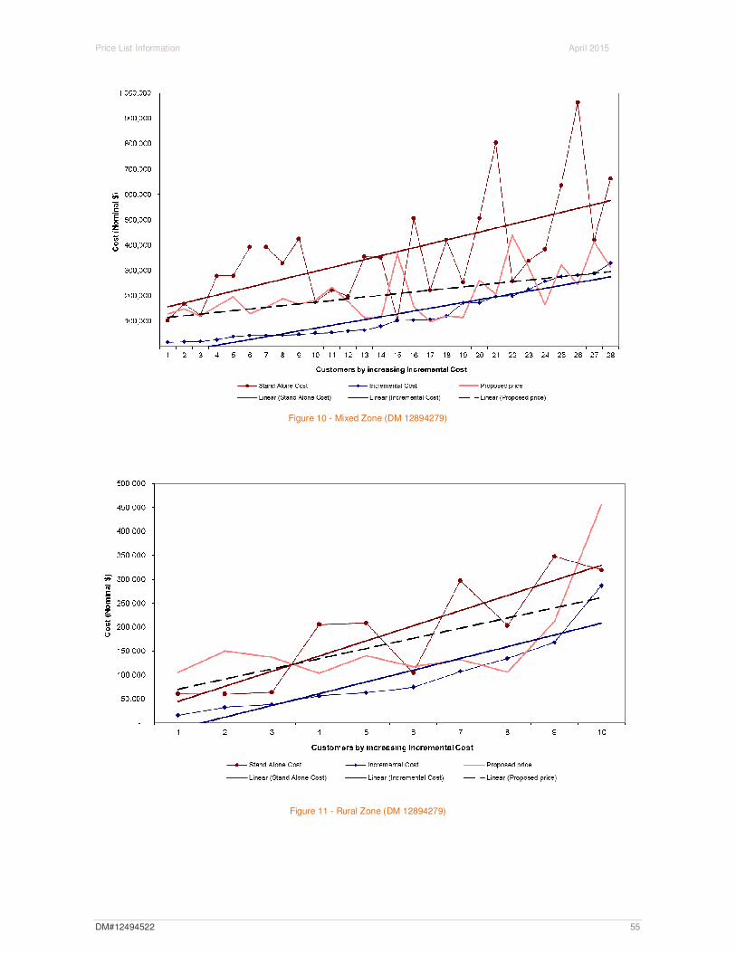
Price List Information April 2015
Figure 10 - Mixed Zone (DM 12894279)
Figure 11 - Rural Zone (DM 12894279)
DM#12494522 55

Price List Information April 2015
7.2.2 Demand/Length Graph
Figure 12 - Demand Length Rates and CMD Rates by Zone (DM 12894279)
7.2.3 Forecast Tariff Revenue
The following table details the forecast distribution reference service revenue, by tariff, which will be collected from distribution connection points.
Table 15 - Distribution Reference Service Revenue Recovered from Distribution Connection Points for 2015/16 ($M Nominal) Forecast
Number Distribution kWh ATMD kVA
Customers Revenue Recovered
RT1 - Anytime Energy (Residential) 5,040,980,245 1,970,869 927,656 636.7
RT2 - Anytime Energy (Business) 1,180,341,029 535,936 85,671 154.8
RT3 - Time of Use Energy (Residential) 159,278,898 63,877 21,594 17.0
RT4 - Time of Use Energy (Business) 1,963,747,971 1,168,543 14,951 164.7
RT5 - High Voltage Metered Demand 363,429,118 111,092 132 14.7
RT6 - Low Voltage Metered Demand 1,642,782,344 486,759 2,479 82.2
RT7 - High Voltage Contract Maximum Demand 3,066,884,986 850,058 285 48.9
RT8 - Low Voltage Contract Maximum Demand 223,356,447 73,246 61 9.1
RT9 – Streetlighting 123,353,806 30,149 248,492 37.0
RT10 - Unmetered Supplies 32,680,258 5,095 15,531 4.1
RT11 - Distribution Entry 0 0 20 2.0
RT13 – Anytime Energy (Residential) Bi-directional 0 0 0 0
RT14 – Anytime Energy (Business) Bi-directional 0 0 0 0
RT15 – Time of Use (Residential) Bi-directional 0 0 0 0
RT16 – Time of Use (Business) Bi-directional 0 0 0 0
TOTAL – Reference Services 13,796,835,102 5,295,623 1,316,872 1,171.2
TOTAL – Non-Reference Services 0.7
TOTAL 1,172.0
DM#12494522
56
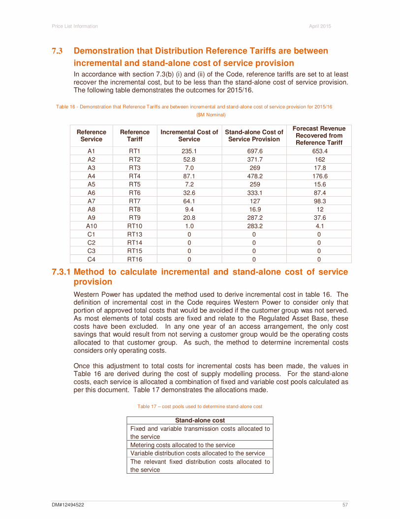
Price List Information April 2015
7.3 Demonstration that Distribution Reference Tariffs are between
incremental and stand-alone cost of service provision
In accordance with section 7.3(b) (i) and (ii) of the Code, reference tariffs are set to at least recover the incremental cost, but to be less than the stand-alone cost of service provision. The following table demonstrates the outcomes for 2015/16.
Table 16 - Demonstration that Reference Tariffs are between incremental and stand-alone cost of service provision for 2015/16
($M Nominal)
Reference Service
Reference Tariff
Incremental Cost of Service
Stand-alone Cost of Service Provision
Forecast Revenue Recovered from Reference Tariff
A1 RT1 235.1 697.6 653.4
A2 RT2 52.8 371.7 162
A3 RT3 7.0 269 17.8
A4 RT4 87.1 478.2 176.6
A5 RT5 7.2 259 15.6
A6 RT6 32.6 333.1 87.4
A7 RT7 64.1 127 98.3
A8 RT8 9.4 16.9 12
A9 RT9 20.8 287.2 37.6
A10 RT10 1.0 283.2 4.1
C1 RT13 0 0 0
C2 RT14 0 0 0
C3 RT15 0 0 0
C4 RT16 0 0 0
7.3.1 Method to calculate incremental and stand-alone cost of service provision
Western Power has updated the method used to derive incremental cost in table 16. The definition of incremental cost in the Code requires Western Power to consider only that portion of approved total costs that would be avoided if the customer group was not served. As most elements of total costs are fixed and relate to the Regulated Asset Base, these costs have been excluded. In any one year of an access arrangement, the only cost savings that would result from not serving a customer group would be the operating costs allocated to that customer group. As such, the method to determine incremental costs considers only operating costs.
Once this adjustment to total costs for incremental costs has been made, the values in Table 16 are derived during the cost of supply modelling process. For the stand-alone costs, each service is allocated a combination of fixed and variable cost pools calculated as per this document. Table 17 demonstrates the allocations made.
Table 17 – cost pools used to determine stand-alone cost
Stand-alone cost
Fixed and variable transmission costs allocated to
the service
Metering costs allocated to the service
Variable distribution costs allocated to the service
The relevant fixed distribution costs allocated to
the service
DM#12494522 57

Price List Information April 2015
7.4 Demonstration that incremental costs are recovered through
variable components
Section 7.6 of the Code states that the incremental cost of service provision should be recovered by the variable components of tariffs. Western Power has had regard to this requirement in setting tariffs. The following table shows that the variable components for 2015/16 tariffs exceeds the incremental cost calculated in section 7.3 for all tariffs.
Table 18 – demonstration that variable costs exceed incremental costs
Reference Service
Reference Tariff
Incremental Cost of Service
Variable tariff
components
A1 RT1 235.1 377.7
A2 RT2 52.8 116.3
A3 RT3 7.0 11.4
A4 RT4 87.1 161.2
A5 RT5 7.2 15.1
A6 RT6 32.6 85.6
A7 RT7 64.1 93.1
A8 RT8 9.4 11.2
A9 RT9 20.8 31.2
A10 RT10 1.0 1.1
7.5 Annual Price Review At the end of each year, the actual distribution reference service revenue entitlement is reconciled against the actual distribution reference service revenue recovered for that year, and an equivalent correction factor is applied to the forecast reference service revenue for the subsequent year. Tariffs are then adjusted to recover the corrected revenue for the following year and the new prices published.
Distribution prices can be volatile due to matters beyond the control of any one user. In order to minimise this volatility and reduce the commercial uncertainty for users, revenues are subject to an annual “side constraint” (effectively a limit on annual reference tariff revenue changes) as detailed in the Access Arrangement. This side constraint will, by extension, have a controlling effect on price movements.
7.6 Tariff Equalisation Contribution (TEC) in the Distribution
Components of Distribution Reference Tariffs
This section details the amounts associated with TEC that are embedded within the distribution reference tariff components.
Western Power pays TEC to the WA State Government to contribute towards maintaining the financial viability of Horizon Power under Part 9A of the Electricity Industry Act 2004. The purpose of TEC is to enable the regulated retail tariffs for electricity that is not supplied from the South West interconnected system (SWIS) to be, so far as is practicable, the same as the regulated retail tariffs for electricity that is supplied from the SWIS.
The graphs and tables detailed in previous sections are inclusive of TEC. The tables that follow in this section separate out the amounts of TEC that are embedded within the distribution reference tariff components.
DM#12494522 58
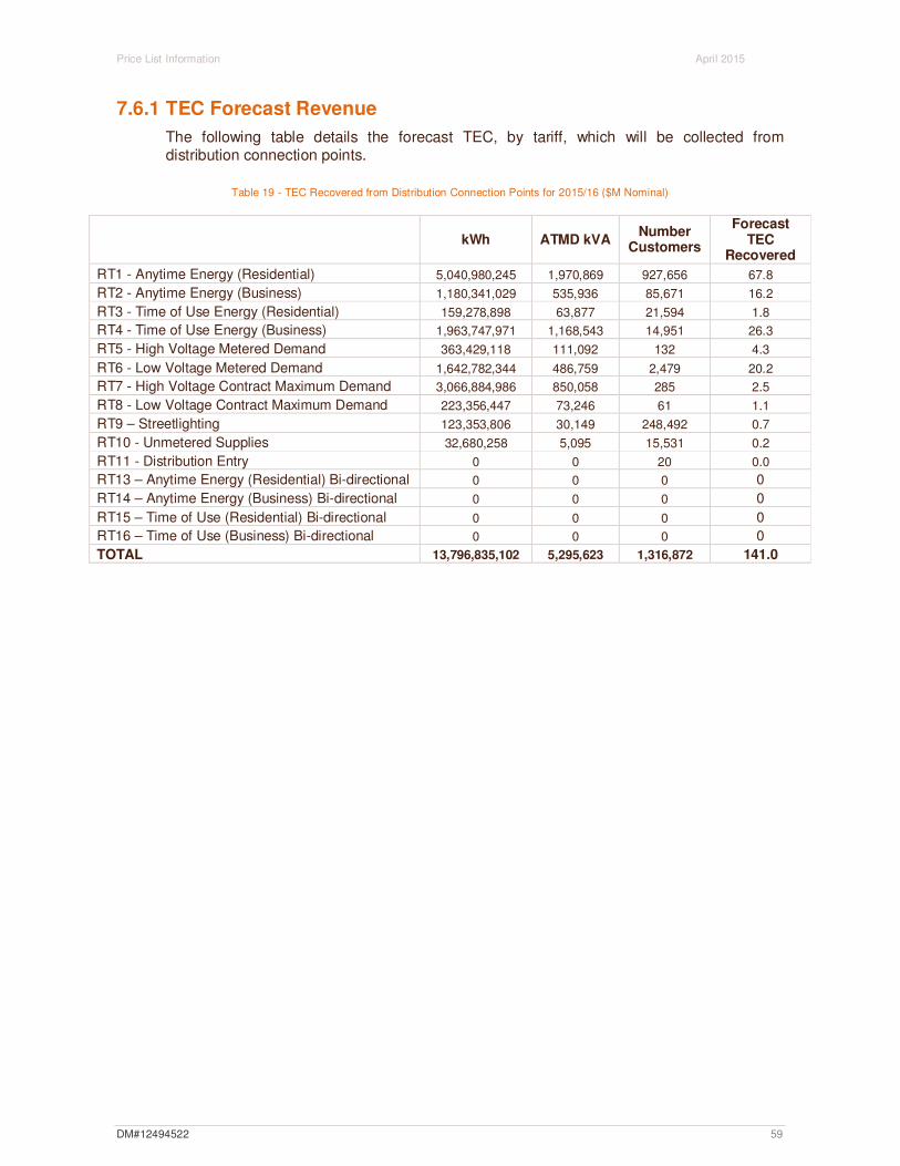
Price List Information April 2015
7.6.1 TEC Forecast Revenue
The following table details the forecast TEC, by tariff, which will be collected from distribution connection points.
Table 19 - TEC Recovered from Distribution Connection Points for 2015/16 ($M Nominal)
kWh ATMD kVA Number
Customers
Forecast TEC
Recovered
RT1 - Anytime Energy (Residential) 5,040,980,245 1,970,869 927,656 67.8
RT2 - Anytime Energy (Business) 1,180,341,029 535,936 85,671 16.2
RT3 - Time of Use Energy (Residential) 159,278,898 63,877 21,594 1.8
RT4 - Time of Use Energy (Business) 1,963,747,971 1,168,543 14,951 26.3
RT5 - High Voltage Metered Demand 363,429,118 111,092 132 4.3
RT6 - Low Voltage Metered Demand 1,642,782,344 486,759 2,479 20.2
RT7 - High Voltage Contract Maximum Demand 3,066,884,986 850,058 285 2.5
RT8 - Low Voltage Contract Maximum Demand 223,356,447 73,246 61 1.1
RT9 – Streetlighting 123,353,806 30,149 248,492 0.7
RT10 - Unmetered Supplies 32,680,258 5,095 15,531 0.2
RT11 - Distribution Entry 0 0 20 0.0
RT13 – Anytime Energy (Residential) Bi-directional 0 0 0 0
RT14 – Anytime Energy (Business) Bi-directional 0 0 0 0
RT15 – Time of Use (Residential) Bi-directional 0 0 0 0
RT16 – Time of Use (Business) Bi-directional 0 0 0 0
TOTAL 13,796,835,102 5,295,623 1,316,872 141.0
DM#12494522 59

Price List Information April 2015
7.6.2 TEC Tariff Components – Use of System
The following table details the amounts associated with TEC that are embedded within the distribution reference tariff use of system components.
Table 20
Fixed TEC Variable TEC
c/day c/kWh On Peak c/kWh
Off Peak c/kWh
Reference tariff 1 RT1 TEC 0.000 1.344 - -
Reference tariff 2 RT2 TEC 0.000 1.376 - -
Reference tariff 3 RT3
TEC 0.000 - 1.960 0.560
Reference tariff 4 RT4
TEC 0.000 - 1.990 0.569
Reference tariff 9 – RT9
TEC 0.000 0.528 - -
Reference tariff 10 – RT10
TEC 0.000 0.509 - -
7.6.3 TEC Tariff Components – Metered Demand
The following table details the amounts associated with TEC that are embedded within the distribution reference tariff metered demand components.
Table 21
RT5 – TEC RT6 – TEC
Demand (kVA)
(Lower to upper
threshold)
Fixed c/day
Demand (in excess of
lower threshold) c/kVA/day
Fixed c/day
Demand (in excess of
lower threshold) c/kVA/day
0 to 300 13.661 14.951 13.661 14.951
300 to 1000 4,498.961 14.423 4,498.961 14.423
1000 to 1500 14,595.061 5.246 14,595.061 5.246
DM#12494522 60
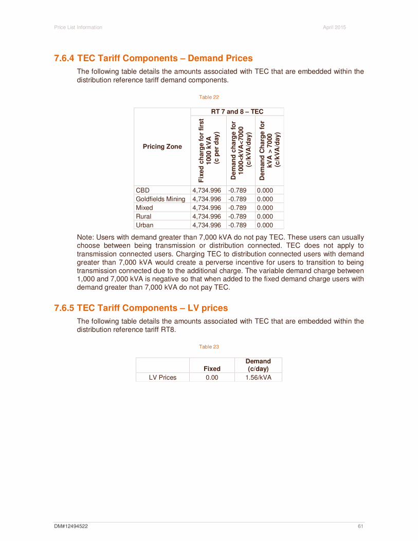
Price List Information April 2015
7.6.4 TEC Tariff Components – Demand Prices
The following table details the amounts associated with TEC that are embedded within the distribution reference tariff demand components.
Table 22
Pricing Zone
RT 7 and 8 – TEC
Fix
ed
ch
arg
e f
or
firs
t1
00
0 k
VA
(c p
er
day
)
De
man
d c
ha
rge f
or
100
0<
kV
A<
70
00
(c/k
VA
/da
y)
De
man
d C
ha
rge f
or
kV
A >
70
00
(c/k
VA
/da
y)
CBD 4,734.996 -0.789 0.000
Goldfields Mining 4,734.996 -0.789 0.000
Mixed 4,734.996 -0.789 0.000
Rural 4,734.996 -0.789 0.000
Urban 4,734.996 -0.789 0.000
Note: Users with demand greater than 7,000 kVA do not pay TEC. These users can usually choose between being transmission or distribution connected. TEC does not apply to transmission connected users. Charging TEC to distribution connected users with demand greater than 7,000 kVA would create a perverse incentive for users to transition to being transmission connected due to the additional charge. The variable demand charge between 1,000 and 7,000 kVA is negative so that when added to the fixed demand charge users with demand greater than 7,000 kVA do not pay TEC.
7.6.5 TEC Tariff Components – LV prices
The following table details the amounts associated with TEC that are embedded within the distribution reference tariff RT8.
Table 23
Demand Fixed (c/day)
LV Prices 0.00 1.56/kVA
DM#12494522 61
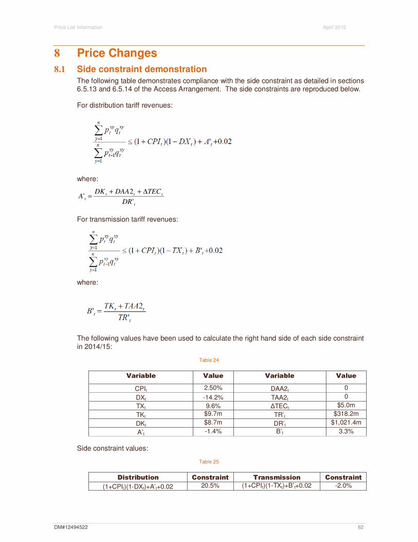
Price List Information April 2015
8 Price Changes
8.1 Side constraint demonstration
The following table demonstrates compliance with the side constraint as detailed in sections 6.5.13 and 6.5.14 of the Access Arrangement. The side constraints are reproduced below.
For distribution tariff revenues:
where:
DK + DAA 2 + ΔTEC t t t
A' = t
DR ' t
For transmission tariff revenues:
where:
The following values have been used to calculate the right hand side of each side constraint in 2014/15:
Table 24
Variable Value Variable Value
CPIt 2.50% DAA2t 0
DXt -14.2% TAA2t 0
TXt 9.6% ∆TECt $5.0m
TKt $9.7m TR’t $318.2m
DKt $8.7m DR’t $1,021.4m
A’t -1.4% B’t 3.3%
Side constraint values:
Table 25
Distribution Constraint Transmission Constraint
(1+CPIt)(1-DXt)+A’t+0.02 20.5% (1+CPIt)(1-TXt)+B’t+0.02 -2.0%
DM#12494522 62

Price List Information April 2015
Table 26 demonstrates compliance with these constraints on all tariffs.
Table 26
Change in weighted average
prices
Constraint compliance
Tariff Distribution Transmission Distribution Transmission
RT1 11% -16% ���� ����
RT2 8% -16% ���� ����
RT3 8% -16% ���� ����
RT4 12% -7% ���� ����
RT5 9% -14% ���� ����
RT6 10% -14% ���� ����
RT7 5% -6% ���� ����
RT8 7% -7% ���� ����
RT9 9% -14% ���� ����
RT10 11% -9% ���� ����
RT11 4% -4% ���� ����
RT13 * * N/A N/A
RT14 * * N/A N/A
RT15 * * N/A N/A
RT16 * * N/A N/A
TRT1 N/A -7% N/A ����
TRT2 N/A -4% N/A ����
*Not applicable as there are no customers on this tariff yet and therefore no revenue.
8.2 Re-balancing of tariffs
The majority of the variations at the tariff level closely follow the average movement of either distribution (10% increase) or transmission (10% decrease). The exceptions to this are:
• TRT1 has a smaller decrease than average due to the commissioning of the Mid West Energy Project slightly changing the allocation of costs between transmission connected users and distribution connected users
• TRT2 has a smaller decrease than average due to similar revenue (proportionally) being collected from less generation capacity (due to retirement of plant)
• RT7 and RT8 movements for distribution are lower than average due to the alternative approach used in setting tariffs (described in Section 7.1.5). The lower transmission decrease is due to these components being driven by the TRT1 prices.
• RT11 takes price movements from RT7 for distribution and TRT2 for transmission.
• Most of the transmission movements for distribution tariffs are larger than average due to less revenue being allocated (proportionally) due to lower demand.
At the tariff component level, there are differing movements on some fixed and variable charges. These movements primarily relate to the reducing energy volumes, combined with increasing customer numbers. The most significant increase to a fixed component occurs on RT4. While the increase to the fixed charge (100%) is large, the resulting fixed charge is still only recovering less than 8% of the total revenue for the tariff.
DM#12494522 63

Price List Information April 2015
8.3 Individual component changes
The following tables detail the % change in the 2015/16 tariff components when compared to the 2014/15 tariff components.
8.3.1 Use of System Prices
The % changes in the following table are applicable for reference tariffs: RT1, RT2, RT3, RT4, RT9, RT10, RT13, RT14, RT15 and RT16.
Table 27
Fixed Price Energy Rates
% Change Anytime %
Change
On Peak
% Change
Off Peak
% Change Reference tariff 1 - RT1
Transmission -15.53%
Distribution 35.50% 0.53%
Bundled Tariff 35.50% -3.29%
Metering 2.71% -17.49% Reference tariff 2 – RT2
Transmission -15.54%
Distribution 39.51% 0.36%
Bundled Tariff 39.51% -3.11%
Metering 2.71% -17.49% Reference tariff 3 - RT3
Transmission -16.31% -16.27%
Distribution 35.50% 0.44% 0.42%
Bundled Tariff 35.50% -3.91% -3.64%
Metering 2.71% -18.63% -18.63% Reference tariff 4 - RT4
Transmission -7.10% -7.04%
Distribution 100.00% 8.29% 8.04%
Bundled Tariff 100.00% 4.72% 4.33%
Metering 2.73% -16.48% -16.48% Reference tariff 9 – RT9
Transmission -13.51%
Distribution 24.00% 6.60%
Bundled Tariff 24.00% 0.95% Reference tariff 10 – RT10
Transmission -8.71%
Distribution 11.15% 10.00%
Bundled Tariff 11.15% 6.44% Reference tariff 13 – RT13
Transmission -15.53%
Distribution 35.50% 0.53%
Bundled Tariff 35.50% -3.29%
Metering 2.71% -17.49%
Reference tariff 14 – RT14
Transmission -15.54%
Distribution 39.51% 0.36%
Bundled Tariff 39.51% -3.11%
Metering 2.71% -17.49%
DM#12494522 64

Price List Information April 2015
Reference tariff 15 – RT15
Transmission -16.31% -16.27%
Distribution 35.50% 0.44% 0.42%
Bundled Tariff 35.50% -3.91% -3.64%
Metering 2.71% -18.63% -18.63% Reference tariff 16 – RT16
Transmission -7.10% -7.04%
Distribution 100.00% 8.29% 8.04%
Bundled Tariff 100.00% 4.72% 4.33%
Metering 2.73% -16.48% -16.48%
8.3.2 Streetlight Asset Prices
The % changes in the following table are applicable for reference tariff: RT9.
Table 28
Light Specification Annual Charge
% Change
42W CFL SE 6.3%
42W CFL BH 6.3%
42W CFL KN 6.3%
70W MH 6.3%
70W HPS 6.3%
125W MV 6.3%
150W MH 6.3%
150W HPS 6.3%
250W MH 6.3%
250W HPS 6.3%
Table 29
Light Specification Annual Charge
% Change
50W MV 6.3%
70W MV 6.3%
80W MV 6.3%
150W MV 6.3%
250W MV 6.3%
400W MV 6.3%
40W FLU 6.3%
80W HPS 6.3%
125W HPS 6.3%
100W INC 6.3%
80W MH 6.3%
125W MH 6.3%
DM#12494522 65
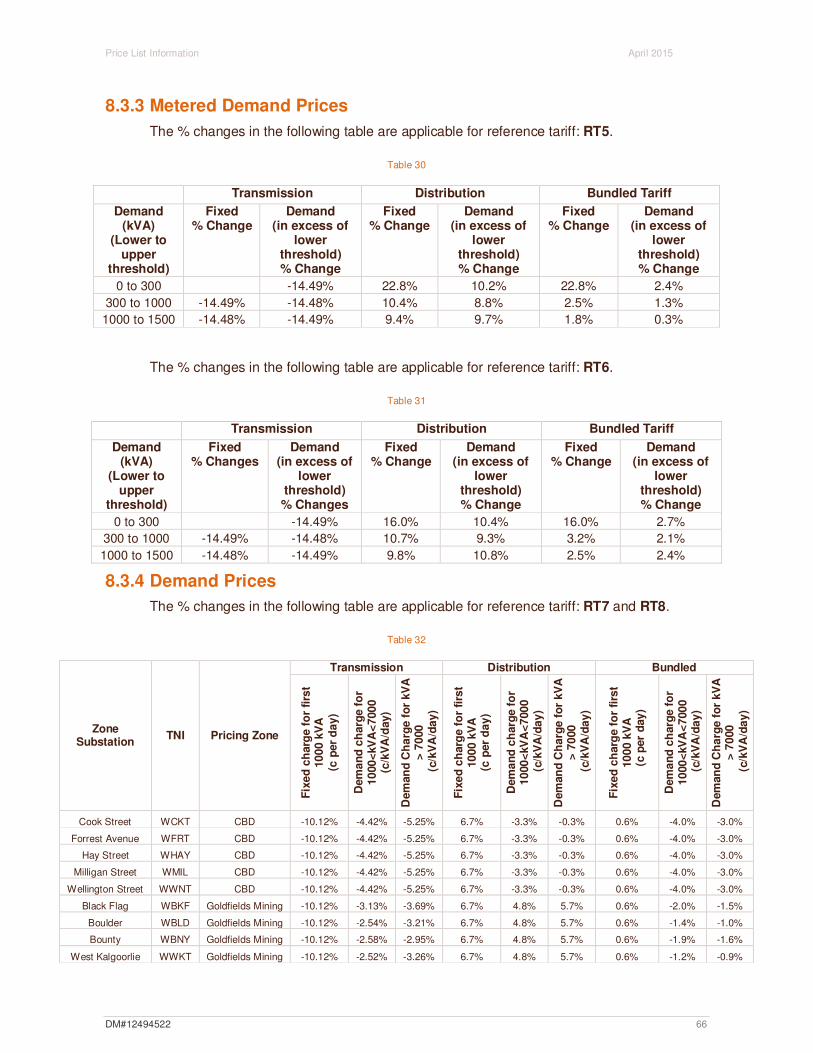
Price List Information April 2015
8.3.3 Metered Demand Prices
The % changes in the following table are applicable for reference tariff: RT5.
Table 30
Transmission Distribution Bundled Tariff
Demand (kVA)
(Lower to upper
threshold)
Fixed % Change
Demand (in excess of
lower threshold) % Change
Fixed % Change
Demand (in excess of
lower threshold) % Change
Fixed % Change
Demand (in excess of
lower threshold) % Change
0 to 300 -14.49% 22.8% 10.2% 22.8% 2.4%
300 to 1000 -14.49% -14.48% 10.4% 8.8% 2.5% 1.3%
1000 to 1500 -14.48% -14.49% 9.4% 9.7% 1.8% 0.3%
The % changes in the following table are applicable for reference tariff: RT6.
Table 31
Transmission Distribution Bundled Tariff
Demand (kVA)
(Lower to upper
threshold)
Fixed % Changes
Demand (in excess of
lower threshold) % Changes
Fixed % Change
Demand (in excess of
lower threshold) % Change
Fixed % Change
Demand (in excess of
lower threshold) % Change
0 to 300 -14.49% 16.0% 10.4% 16.0% 2.7%
300 to 1000 -14.49% -14.48% 10.7% 9.3% 3.2% 2.1%
1000 to 1500 -14.48% -14.49% 9.8% 10.8% 2.5% 2.4%
8.3.4 Demand Prices
The % changes in the following table are applicable for reference tariff: RT7 and RT8.
Table 32
Zone Substation
TNI Pricing Zone
Transmission Distribution Bundled
Fix
ed
ch
arg
e f
or
firs
t10
00
kV
A(c
per
da
y)
Dem
an
d c
harg
e f
or
10
00
<kV
A<
700
0(c
/kV
A/d
ay)
Dem
an
d C
ha
rge
fo
r kV
A>
70
00
(c/k
VA
/da
y)
Fix
ed
ch
arg
e f
or
firs
t10
00
kV
A(c
per
da
y)
Dem
an
d c
harg
e f
or
10
00
<kV
A<
700
0(c
/kV
A/d
ay
)
Dem
an
d C
ha
rge
fo
r kV
A>
70
00
(c/k
VA
/da
y)
Fix
ed
ch
arg
e f
or
firs
t10
00
kV
A(c
per
day
)
Dem
an
d c
harg
e f
or
10
00
<kV
A<
700
0(c
/kV
A/d
ay
)
Dem
an
d C
ha
rge
fo
r kV
A>
70
00
(c/k
VA
/da
y)
Cook Street WCKT CBD -10.12% -4.42% -5.25% 6.7% -3.3% -0.3% 0.6% -4.0% -3.0%
Forrest Avenue WFRT CBD -10.12% -4.42% -5.25% 6.7% -3.3% -0.3% 0.6% -4.0% -3.0%
Hay Street WHAY CBD -10.12% -4.42% -5.25% 6.7% -3.3% -0.3% 0.6% -4.0% -3.0%
Milligan Street WMIL CBD -10.12% -4.42% -5.25% 6.7% -3.3% -0.3% 0.6% -4.0% -3.0%
Wellington Street WWNT CBD -10.12% -4.42% -5.25% 6.7% -3.3% -0.3% 0.6% -4.0% -3.0%
Black Flag WBKF Goldfields Mining -10.12% -3.13% -3.69% 6.7% 4.8% 5.7% 0.6% -2.0% -1.5%
Boulder WBLD Goldfields Mining -10.12% -2.54% -3.21% 6.7% 4.8% 5.7% 0.6% -1.4% -1.0%
Bounty WBNY Goldfields Mining -10.12% -2.58% -2.95% 6.7% 4.8% 5.7% 0.6% -1.9% -1.6%
West Kalgoorlie WWKT Goldfields Mining -10.12% -2.52% -3.26% 6.7% 4.8% 5.7% 0.6% -1.2% -0.9%
DM#12494522 66
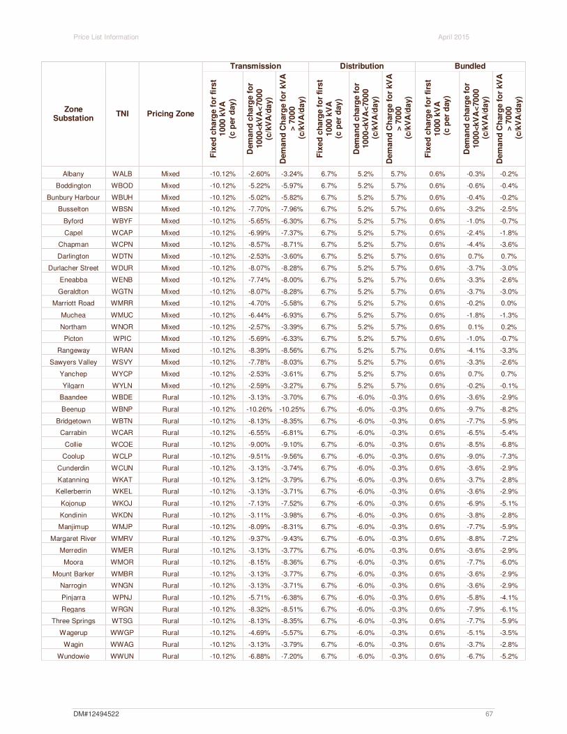
Price List Information April 2015
Zone Substation
TNI Pricing Zone
Transmission Distribution Bundled
Fix
ed
ch
arg
e f
or
firs
t1
000
kV
A(c
per
day
)
Dem
an
d c
ha
rge
fo
r10
00
<kV
A<
70
00
(c/k
VA
/da
y)
Dem
an
d C
harg
e f
or
kV
A>
70
00
(c/k
VA
/da
y)
Fix
ed
ch
arg
e f
or
firs
t1
000
kV
A(c
per
day
)
Dem
an
d c
ha
rge
fo
r10
00
<kV
A<
70
00
(c/k
VA
/da
y)
Dem
an
d C
harg
e f
or
kV
A>
70
00
(c/k
VA
/da
y)
Fix
ed
ch
arg
e f
or
firs
t1
000
kV
A(c
per
day
)
Dem
an
d c
ha
rge
fo
r10
00
<kV
A<
70
00
(c/k
VA
/da
y)
Dem
an
d C
harg
e f
or
kV
A>
70
00
(c/k
VA
/da
y)
Albany WALB Mixed -10.12% -2.60% -3.24% 6.7% 5.2% 5.7% 0.6% -0.3% -0.2%
Boddington WBOD Mixed -10.12% -5.22% -5.97% 6.7% 5.2% 5.7% 0.6% -0.6% -0.4%
Bunbury Harbour WBUH Mixed -10.12% -5.02% -5.82% 6.7% 5.2% 5.7% 0.6% -0.4% -0.2%
Busselton WBSN Mixed -10.12% -7.70% -7.96% 6.7% 5.2% 5.7% 0.6% -3.2% -2.5%
Byford WBYF Mixed -10.12% -5.65% -6.30% 6.7% 5.2% 5.7% 0.6% -1.0% -0.7%
Capel WCAP Mixed -10.12% -6.99% -7.37% 6.7% 5.2% 5.7% 0.6% -2.4% -1.8%
Chapman WCPN Mixed -10.12% -8.57% -8.71% 6.7% 5.2% 5.7% 0.6% -4.4% -3.6%
Darlington WDTN Mixed -10.12% -2.53% -3.60% 6.7% 5.2% 5.7% 0.6% 0.7% 0.7%
Durlacher Street WDUR Mixed -10.12% -8.07% -8.28% 6.7% 5.2% 5.7% 0.6% -3.7% -3.0%
Eneabba WENB Mixed -10.12% -7.74% -8.00% 6.7% 5.2% 5.7% 0.6% -3.3% -2.6%
Geraldton WGTN Mixed -10.12% -8.07% -8.28% 6.7% 5.2% 5.7% 0.6% -3.7% -3.0%
Marriott Road WMRR Mixed -10.12% -4.70% -5.58% 6.7% 5.2% 5.7% 0.6% -0.2% 0.0%
Muchea WMUC Mixed -10.12% -6.44% -6.93% 6.7% 5.2% 5.7% 0.6% -1.8% -1.3%
Northam WNOR Mixed -10.12% -2.57% -3.39% 6.7% 5.2% 5.7% 0.6% 0.1% 0.2%
Picton WPIC Mixed -10.12% -5.69% -6.33% 6.7% 5.2% 5.7% 0.6% -1.0% -0.7%
Rangeway WRAN Mixed -10.12% -8.39% -8.56% 6.7% 5.2% 5.7% 0.6% -4.1% -3.3%
Sawyers Valley WSVY Mixed -10.12% -7.78% -8.03% 6.7% 5.2% 5.7% 0.6% -3.3% -2.6%
Yanchep WYCP Mixed -10.12% -2.53% -3.61% 6.7% 5.2% 5.7% 0.6% 0.7% 0.7%
Yilgarn WYLN Mixed -10.12% -2.59% -3.27% 6.7% 5.2% 5.7% 0.6% -0.2% -0.1%
Baandee WBDE Rural -10.12% -3.13% -3.70% 6.7% -6.0% -0.3% 0.6% -3.6% -2.9%
Beenup WBNP Rural -10.12% -10.26% -10.25% 6.7% -6.0% -0.3% 0.6% -9.7% -8.2%
Bridgetown WBTN Rural -10.12% -8.13% -8.35% 6.7% -6.0% -0.3% 0.6% -7.7% -5.9%
Carrabin WCAR Rural -10.12% -6.55% -6.81% 6.7% -6.0% -0.3% 0.6% -6.5% -5.4%
Collie WCOE Rural -10.12% -9.00% -9.10% 6.7% -6.0% -0.3% 0.6% -8.5% -6.8%
Coolup WCLP Rural -10.12% -9.51% -9.56% 6.7% -6.0% -0.3% 0.6% -9.0% -7.3%
Cunderdin WCUN Rural -10.12% -3.13% -3.74% 6.7% -6.0% -0.3% 0.6% -3.6% -2.9%
Katanning WKAT Rural -10.12% -3.12% -3.79% 6.7% -6.0% -0.3% 0.6% -3.7% -2.8%
Kellerberrin WKEL Rural -10.12% -3.13% -3.71% 6.7% -6.0% -0.3% 0.6% -3.6% -2.9%
Kojonup WKOJ Rural -10.12% -7.13% -7.52% 6.7% -6.0% -0.3% 0.6% -6.9% -5.1%
Kondinin WKDN Rural -10.12% -3.11% -3.98% 6.7% -6.0% -0.3% 0.6% -3.8% -2.8%
Manjimup WMJP Rural -10.12% -8.09% -8.31% 6.7% -6.0% -0.3% 0.6% -7.7% -5.9%
Margaret River WMRV Rural -10.12% -9.37% -9.43% 6.7% -6.0% -0.3% 0.6% -8.8% -7.2%
Merredin WMER Rural -10.12% -3.13% -3.77% 6.7% -6.0% -0.3% 0.6% -3.6% -2.9%
Moora WMOR Rural -10.12% -8.15% -8.36% 6.7% -6.0% -0.3% 0.6% -7.7% -6.0%
Mount Barker WMBR Rural -10.12% -3.13% -3.77% 6.7% -6.0% -0.3% 0.6% -3.6% -2.9%
Narrogin WNGN Rural -10.12% -3.13% -3.71% 6.7% -6.0% -0.3% 0.6% -3.6% -2.9%
Pinjarra WPNJ Rural -10.12% -5.71% -6.38% 6.7% -6.0% -0.3% 0.6% -5.8% -4.1%
Regans WRGN Rural -10.12% -8.32% -8.51% 6.7% -6.0% -0.3% 0.6% -7.9% -6.1%
Three Springs WTSG Rural -10.12% -8.13% -8.35% 6.7% -6.0% -0.3% 0.6% -7.7% -5.9%
Wagerup WWGP Rural -10.12% -4.69% -5.57% 6.7% -6.0% -0.3% 0.6% -5.1% -3.5%
Wagin WWAG Rural -10.12% -3.13% -3.79% 6.7% -6.0% -0.3% 0.6% -3.7% -2.8%
Wundowie WWUN Rural -10.12% -6.88% -7.20% 6.7% -6.0% -0.3% 0.6% -6.7% -5.2%
DM#12494522 67

Price List Information April 2015
Zone Substation
TNI Pricing Zone
Transmission Distribution Bundled
Fix
ed
ch
arg
e f
or
firs
t1
000
kV
A(c
per
day
)
Dem
an
d c
ha
rge
fo
r10
00
<kV
A<
70
00
(c/k
VA
/da
y)
Dem
an
d C
harg
e f
or
kV
A>
70
00
(c/k
VA
/da
y)
Fix
ed
ch
arg
e f
or
firs
t1
000
kV
A(c
per
day
)
Dem
an
d c
ha
rge
fo
r10
00
<kV
A<
70
00
(c/k
VA
/da
y)
Dem
an
d C
harg
e f
or
kV
A>
70
00
(c/k
VA
/da
y)
Fix
ed
ch
arg
e f
or
firs
t1
000
kV
A(c
per
day
)
Dem
an
d c
ha
rge
fo
r10
00
<kV
A<
70
00
(c/k
VA
/da
y)
Dem
an
d C
harg
e f
or
kV
A>
70
00
(c/k
VA
/da
y)
Yerbillon WYER Rural -10.12% -6.51% -6.78% 6.7% -6.0% -0.3% 0.6% -6.4% -5.3%
Amherst WAMT Urban -10.12% -4.15% -5.00% 6.7% 3.3% 5.6% 0.6% -3.3% -2.2%
Arkana WARK Urban -10.12% -4.15% -5.00% 6.7% 3.3% 5.6% 0.6% -3.3% -2.2%
Australian Paper
Mills
WAPM Urban -10.12% -4.15% -5.00% 6.7% 3.3% 5.6% 0.6% -3.3% -2.2%
Balcatta WBCT Urban -10.12% -4.15% -5.00% 6.7% 3.3% 5.6% 0.6% -3.3% -2.2%
Beechboro WBCH Urban -10.12% -4.15% -5.00% 6.7% 3.3% 5.6% 0.6% -3.3% -2.2%
Belmont WBEL Urban -10.12% -4.15% -5.00% 6.7% 3.3% 5.6% 0.6% -3.3% -2.2%
Bentley WBTY Urban -10.12% -4.15% -5.00% 6.7% 3.3% 5.6% 0.6% -3.3% -2.2%
Bibra Lake WBIB Urban -10.12% -4.15% -5.00% 6.7% 3.3% 5.6% 0.6% -3.3% -2.2%
British Petroleum WBPM Urban -10.12% -4.15% -5.00% 6.7% 3.3% 5.6% 0.6% -3.3% -2.2%
Canning Vale WCVE Urban -10.12% -4.15% -5.00% 6.7% 3.3% 5.6% 0.6% -3.3% -2.2%
Clarence Street WCLN Urban -10.12% -4.15% -5.00% 6.7% 3.3% 5.6% 0.6% -3.3% -2.2%
Clarkson WCKN Urban -10.12% -4.15% -5.00% 6.7% 3.3% 5.6% 0.6% -3.3% -2.2%
Cockburn Cement WCCT Urban -10.12% -4.15% -5.00% 6.7% 3.3% 5.6% 0.6% -3.3% -2.2%
Collier WCOL Urban -10.12% -4.15% -5.00% 6.7% 3.3% 5.6% 0.6% -3.3% -2.2%
Cottesloe WCTE Urban -10.12% -4.15% -5.00% 6.7% 3.3% 5.6% 0.6% -3.3% -2.2%
Edmund Street WEDD Urban -10.12% -4.15% -5.00% 6.7% 3.3% 5.6% 0.6% -3.3% -2.2%
Forrestfield WFFD Urban -10.12% -4.15% -5.00% 6.7% 3.3% 5.6% 0.6% -3.3% -2.2%
Gosnells WGNL Urban -10.12% -4.15% -5.00% 6.7% 3.3% 5.6% 0.6% -3.3% -2.2%
Hadfields WHFS Urban -10.12% -4.15% -5.00% 6.7% 3.3% 5.6% 0.6% -3.3% -2.2%
Hazelmere WHZM Urban -10.12% -4.15% -5.00% 6.7% 3.3% 5.6% 0.6% -3.3% -2.2%
Henley Brook WHBK Urban -10.12% -4.15% -5.00% 6.7% 3.3% 5.6% 0.6% -3.3% -2.2%
Herdsman Parade WHEP Urban -10.12% -4.15% -5.00% 6.7% 3.3% 5.6% 0.6% -3.3% -2.2%
Joel Terrace WJTE Urban -10.12% -4.15% -5.00% 6.7% 3.3% 5.6% 0.6% -3.3% -2.2%
Joondalup WJDP Urban -10.12% -4.15% -5.00% 6.7% 3.3% 5.6% 0.6% -3.3% -2.2%
Kalamunda WKDA Urban -10.12% -4.15% -5.00% 6.7% 3.3% 5.6% 0.6% -3.3% -2.2%
Kambalda WKBA Urban -10.12% -2.77% -3.42% 6.7% 3.3% 5.6% 0.6% -2.3% -1.7%
Kewdale WKDL Urban -10.12% -4.15% -5.00% 6.7% 3.3% 5.6% 0.6% -3.3% -2.2%
Landsdale WLDE Urban -10.12% -4.15% -5.00% 6.7% 3.3% 5.6% 0.6% -3.3% -2.2%
Maddington WMDN Urban -10.12% -4.15% -5.00% 6.7% 3.3% 5.6% 0.6% -3.3% -2.2%
Malaga WMLG Urban -10.12% -4.15% -5.00% 6.7% 3.3% 5.6% 0.6% -3.3% -2.2%
Mandurah WMHA Urban -10.12% -4.15% -5.00% 6.7% 3.3% 5.6% 0.6% -3.3% -2.2%
Manning Street WMAG Urban -10.12% -4.15% -5.00% 6.7% 3.3% 5.6% 0.6% -3.3% -2.2%
Mason Road WMSR Urban -10.12% -4.15% -5.00% 6.7% 3.3% 5.6% 0.6% -3.3% -2.2%
Meadow Springs WMSS Urban -10.12% -4.15% -5.00% 6.7% 3.3% 5.6% 0.6% -3.3% -2.2%
Medical Centre WMCR Urban -10.12% -4.15% -5.00% 6.7% 3.3% 5.6% 0.6% -3.3% -2.2%
Medina WMED Urban -10.12% -4.15% -5.00% 6.7% 3.3% 5.6% 0.6% -3.3% -2.2%
Midland Junction WMJX Urban -10.12% -4.15% -5.00% 6.7% 3.3% 5.6% 0.6% -3.3% -2.2%
Morley WMOY Urban -10.12% -4.15% -5.00% 6.7% 3.3% 5.6% 0.6% -3.3% -2.2%
Mullaloo WMUL Urban -10.12% -4.15% -5.00% 6.7% 3.3% 5.6% 0.6% -3.3% -2.2%
Mundaring Weir WMWR Urban -10.12% -4.15% -5.00% 6.7% 3.3% 5.6% 0.6% -3.3% -2.2%
DM#12494522 68

Price List Information April 2015
Zone Substation
TNI Pricing Zone
Transmission Distribution Bundled
Fix
ed
ch
arg
e f
or
firs
t1
000
kV
A(c
per
day
)
Dem
an
d c
ha
rge
fo
r10
00
<kV
A<
70
00
(c/k
VA
/da
y)
Dem
an
d C
harg
e f
or
kV
A>
70
00
(c/k
VA
/da
y)
Fix
ed
ch
arg
e f
or
firs
t1
000
kV
A(c
per
day
)
Dem
an
d c
ha
rge
fo
r10
00
<kV
A<
70
00
(c/k
VA
/da
y)
Dem
an
d C
harg
e f
or
kV
A>
70
00
(c/k
VA
/da
y)
Fix
ed
ch
arg
e f
or
firs
t1
000
kV
A(c
per
day
)
Dem
an
d c
ha
rge
fo
r10
00
<kV
A<
70
00
(c/k
VA
/da
y)
Dem
an
d C
harg
e f
or
kV
A>
70
00
(c/k
VA
/da
y)
Munday WMDY Urban -10.12% -4.15% -5.00% 6.7% 3.3% 5.6% 0.6% -3.3% -2.2%
Murdoch WMUR Urban -10.12% -4.15% -5.00% 6.7% 3.3% 5.6% 0.6% -3.3% -2.2%
Myaree WMYR Urban -10.12% -4.15% -5.00% 6.7% 3.3% 5.6% 0.6% -3.3% -2.2%
Nedlands WNED Urban -10.12% -4.15% -5.00% 6.7% 3.3% 5.6% 0.6% -3.3% -2.2%
North Beach WNBH Urban -10.12% -4.15% -5.00% 6.7% 3.3% 5.6% 0.6% -3.3% -2.2%
North Fremantle WNFL Urban -10.12% -4.15% -5.00% 6.7% 3.3% 5.6% 0.6% -3.3% -2.2%
North Perth WNPH Urban -10.12% -4.15% -5.00% 6.7% 3.3% 5.6% 0.6% -3.3% -2.2%
O'Connor WOCN Urban -10.12% -4.15% -5.00% 6.7% 3.3% 5.6% 0.6% -3.3% -2.2%
Osborne Park WOPK Urban -10.12% -4.15% -5.00% 6.7% 3.3% 5.6% 0.6% -3.3% -2.2%
Padbury WPBY Urban -10.12% -4.15% -5.00% 6.7% 3.3% 5.6% 0.6% -3.3% -2.2%
Piccadilly WPCY Urban -10.12% -2.76% -3.45% 6.7% 3.3% 5.6% 0.6% -2.3% -1.7%
Riverton WRTN Urban -10.12% -4.15% -5.00% 6.7% 3.3% 5.6% 0.6% -3.3% -2.2%
Rivervale WRVE Urban -10.12% -4.15% -5.00% 6.7% 3.3% 5.6% 0.6% -3.3% -2.2%
Rockingham WROH Urban -10.12% -4.15% -5.00% 6.7% 3.3% 5.6% 0.6% -3.3% -2.2%
Shenton Park WSPA Urban -10.12% -4.15% -5.00% 6.7% 3.3% 5.6% 0.6% -3.3% -2.2%
Sth Ftle Power
Station
WSFT Urban -10.12% -4.15% -5.00% 6.7% 3.3% 5.6% 0.6% -3.3% -2.2%
Southern River WSNR Urban -10.12% -4.15% -5.00% 6.7% 3.3% 5.6% 0.6% -3.3% -2.2%
Tate Street WTTS Urban -10.12% -4.15% -5.00% 6.7% 3.3% 5.6% 0.6% -3.3% -2.2%
University WUNI Urban -10.12% -4.15% -5.00% 6.7% 3.3% 5.6% 0.6% -3.3% -2.2%
Victoria Park WVPA Urban -10.12% -4.15% -5.00% 6.7% 3.3% 5.6% 0.6% -3.3% -2.2%
Waikiki WWAI Urban -10.12% -4.15% -5.00% 6.7% 3.3% 5.6% 0.6% -3.3% -2.2%
Wangara WWGA Urban -10.12% -4.15% -5.00% 6.7% 3.3% 5.6% 0.6% -3.3% -2.2%
Wanneroo WWNO Urban -10.12% -4.15% -5.00% 6.7% 3.3% 5.6% 0.6% -3.3% -2.2%
Welshpool WWEL Urban -10.12% -4.15% -5.00% 6.7% 3.3% 5.6% 0.6% -3.3% -2.2%
Wembley Downs WWDN Urban -10.12% -4.15% -5.00% 6.7% 3.3% 5.6% 0.6% -3.3% -2.2%
Willetton WWLN Urban -10.12% -4.15% -5.00% 6.7% 3.3% 5.6% 0.6% -3.3% -2.2%
Yokine WYKE Urban -10.12% -4.15% -5.00% 6.7% 3.3% 5.6% 0.6% -3.3% -2.2%
DM#12494522 69
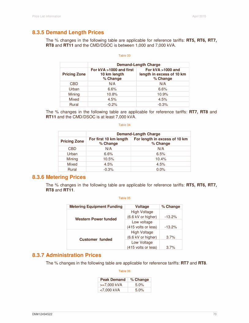
Price List Information April 2015
8.3.5 Demand Length Prices
The % changes in the following table are applicable for reference tariffs: RT5, RT6, RT7, RT8 and RT11 and the CMD/DSOC is between 1,000 and 7,000 kVA.
Table 33
Demand-Length Charge
Pricing Zone For kVA >1000 and first
10 km length % Change
For kVA >1000 and length in excess of 10 km
% Change
CBD N/A N/A
Urban 6.6% 6.6%
Mining 10.8% 10.9%
Mixed 4.5% 4.5%
Rural -0.2% -0.3%
The % changes in the following table are applicable for reference tariffs: RT7, RT8 and RT11 and the CMD/DSOC is at least 7,000 kVA.
Table 34
Demand-Length Charge
Pricing Zone For first 10 km length
% Change For length in excess of 10 km
% Change
CBD N/A N/A
Urban 6.6% 6.5%
Mining 10.5% 10.4%
Mixed 4.5% 4.5%
Rural -0.3% 0.0%
8.3.6 Metering Prices
The % changes in the following table are applicable for reference tariffs: RT5, RT6, RT7, RT8 and RT11.
Table 35
Metering Equipment Funding Voltage % Change
Western Power funded
High Voltage
(6.6 kV or higher) -13.2%
Low voltage
(415 volts or less) -13.2%
Customer funded
High Voltage
(6.6 kV or higher) 3.7%
Low Voltage
(415 volts or less) 3.7%
8.3.7 Administration Prices
The % changes in the following table are applicable for reference tariffs: RT7 and RT8.
Table 36
Peak Demand % Change
>=7,000 kVA 5.0%
<7,000 kVA 5.0%
DM#12494522 70

Price List Information April 2015
8.3.8 Low Voltage Prices
The % changes in the following table are applicable for reference tariff: RT8.
Table 37
Category % Change
Fixed 9.40%
Demand 10.1%
8.3.9 Connection Prices
The % changes in the following table are applicable for reference tariff: RT11.
Table 38
Connection Price % Change
Connection Price -6.3%
8.3.10 Transmission Use of System Prices
The % changes in the following table are applicable for reference tariff: TRT1.
Table 39
Substation TNI Use of System Price
% Change
Albany WALB -4%
Alcoa Pinjarra WAPJ -14%
Amherst WAMT -4%
Arkana WARK -4%
Australian Fused Materials WAFM -4%
Australian Paper Mills WAPM -14%
Baandee (WC) WBDE -4%
Balcatta WBCT -4%
Beckenham WBEC -9%
Beechboro WBCH -4%
Beenup WBNP -14%
Belmont WBEL -6%
Bentley WBTY -12%
Bibra Lake WBIB -14%
Binningup Desalination Plant WBDP -14%
Black Flag WBKF -5%
Boddington Gold Mine WBGM -14%
Boddington WBOD -14%
Boulder WBLD -4%
Bounty WBNY -4%
Bridgetown WBTN -14%
British Petroleum WBPM -4%
Broken Hill Kwinana WBHK -4%
Bunbury Harbour WBUH -14%
Busselton WBSN -14%
Byford WBYF -14%
Canning Vale WCVE -4%
DM#12494522 71

Price List Information April 2015
Substation TNI Use of System Price
% Change
Capel WCAP -14%
Carrabin WCAR -9%
Cataby Kerr McGee WKMC -14%
Chapman WCPN -14%
Clarence Street WCLN -14%
Clarkson WCKN -4%
Cockburn Cement WCCT -14%
Cockburn Cement Ltd WCCL -14%
Collie WCOE -14%
Collier WCOL -14%
Cook Street WCKT -4%
Coolup WCLP -14%
Cottesloe WCTE -4%
Cunderdin WCUN -4%
Darlington WDTN -4%
Edgewater WEDG -4%
Edmund Street WEDD -14%
Eneabba WENB -14%
Forrest Ave WFRT -14%
Forrestfield WFFD -4%
Geraldton WGTN -14%
Glen Iris WGNI -14%
Golden Grove WGGV -14%
Gosnells WGNL -4%
Hadfields WHFS -4%
Hay Street WHAY -11%
Hazelmere WHZM -4%
Henley Brook WHBK -14%
Herdsman Parade WHEP -14%
Joel Terrace WJTE -14%
Joondalup WJDP -4%
Kalamunda WKDA -4%
Katanning WKAT -4%
Kellerberrin WKEL -4%
Kewdale WKDL -4%
Kojonup WKOJ -14%
Kondinin WKDN -4%
Kwinana Alcoa WAKW -4%
Kwinana Desalination Plant WKDP -4%
Kwinana PWS WKPS -14%
Landsdale WLDE -4%
Maddington WMDN -9%
Malaga WMLG -4%
Mandurah WMHA -14%
Manjimup WMJP -14%
Manning Street WMAG -4%
Margaret River WMRV -14%
Marriott Road Barrack Silicon Smelter WBSI -14%
Marriott Road WMRR -14%
Mason Road WMSR -4%
DM#12494522 72

Price List Information April 2015
Substation TNI Use of System Price
% Change
Mason Road CSBP WCBP -14%
Mason Road Kerr McGee WKMK -7%
Meadow Springs WMSS -4%
Medical Centre WMCR -14%
Medina WMED -4%
Merredin 66kV WMER -4%
Midland Junction WMJX -4%
Milligan Street WMIL -14%
Moora WMOR -14%
Morley WMOY -9%
Mt Barker WMBR -4%
Muchea Kerr McGee WKMM -14%
Muchea WMUC -14%
Muja PWS WMPS -7%
Mullaloo WMUL -4%
Munday WMDY -5%
Murdoch WMUR -4%
Mundaring Weir WMWR -14%
Myaree WMYR -14%
Narrogin WNGN -4%
Nedlands WNED -14%
North Beach WNBH -4%
North Fremantle WNFL -14%
North Perth WNPH -4%
Northam WNOR -4%
Nowgerup WNOW N/A
O'Connor WOCN -14%
Osborne Park WOPK -4%
Padbury WPBY -4%
Parkeston WPRK -4%
Parklands WPLD -4%
Piccadilly WPCY -4%
Picton 66kv WPIC -14%
Pinjarra WPNJ -14%
Rangeway WRAN -14%
Regans WRGN -14%
Riverton WRTN -4%
Rivervale WRVE -14%
Rockingham WROH -4%
Sawyers Valley WSVY -14%
Shenton Park WSPA -14%
Southern River WSNR -11%
South Fremantle 22kV WSFT -14%
Summer St WSUM -14%
Sutherland WSRD N/A
Tate Street WTTS -14%
Three Springs WTSG -14%
Three Springs Terminal WTST N/A
Tomlinson Street WTLN -14%
University WUNI -14%
DM#12494522 73
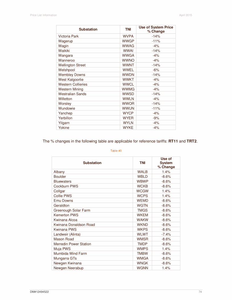
Price List Information April 2015
Substation TNI Use of System Price
% Change
Victoria Park WVPA -14%
Wagerup WWGP -11%
Wagin WWAG -4%
Waikiki WWAI -14%
Wangara WWGA -4%
Wanneroo WWNO -4%
Wellington Street WWNT -14%
Welshpool WWEL -6%
Wembley Downs WWDN -14%
West Kalgoorlie WWKT -4%
Western Collieries WWCL -4%
Western Mining WWMG -4%
Westralian Sands WWSD -14%
Willetton WWLN -4%
Worsley WWOR -14%
Wundowie WWUN -11%
Yanchep WYCP -4%
Yerbillon WYER -9%
Yilgarn WYLN -4%
Yokine WYKE -4%
The % changes in the following table are applicable for reference tariffs: RT11 and TRT2.
Table 40
Substation TNI Use of System
% Change
Albany WALB 1.4%
Boulder WBLD -8.6%
Bluewaters WBWP -8.6%
Cockburn PWS WCKB -8.6%
Collgar WCGW 1.4%
Collie PWS WCPS 1.4%
Emu Downs WEMD -8.6%
Geraldton WGTN -8.6%
Greenough Solar Farm TMGS -8.6%
Kemerton PWS WKEM -8.6%
Kwinana Alcoa WAKW -8.6%
Kwinana Donaldson Road WKND -8.6%
Kwinana PWS WKPS -8.6%
Landweir (Alinta) WLWT -7.4%
Mason Road WMSR -8.6%
Merredin Power Station TMDP -8.6%
Muja PWS WMPS 1.4%
Mumbida Wind Farm TMBW -8.6%
Mungarra GTs WMGA -8.6%
Newgen Kwinana WNGK -8.6%
Newgen Neerabup WGNN 1.4%
DM#12494522 74

Price List Information April 2015
Substation TNI Use of System
% Change
Oakley (Alinta) WOLY -8.6%
Parkeston WPKS -8.6%
Pinjar GTs WPJR -8.6%
Alcoa Pinjarra WAPJ -8.6%
Tiwest GT WKMK -8.6%
Wagerup WWGP -8.6%
Walkaway Windfarm WWWF -8.6%
West Kalgoorlie GTs WWKT -8.6%
Worsley WWOR -8.6%
8.3.11 Common Service Prices
The % changes in the following table are applicable for reference tariff: TRT1.
Table 41
Common Service Price % Change
Common Service Price -7.4%
8.3.12 Control System Service Prices
The % changes in the following table are applicable for reference tariff: RT11 and TRT2.
Table 42
Price % Change
Control System Service Price (Generators) 8.7%
The % changes in the following table are applicable for reference tariff: TRT1.
Table 43
Price % Change
Control System Service Price (Loads) 11.8%
8.3.13 Metering Prices
The % changes in the following table are applicable for reference tariffs: TRT1 and TRT2.
Table 44
% Change
Transmission Metering 0%
DM#12494522 75

Price List Information April 2015
Appendix A - Price Setting for New Transmission Nodes Policy This policy applies when a new transmission node is established.
Transmission “use of system” prices for both entry and exit points are derived using the computer based analysis tool T-Price, based on historical load flow information. In the case of new sites, historical data is not available.
However, there is a need for both Western Power and the prospective user to have a fairly accurate TUOS price and connection price. Western Power requires the prices to determine future revenues from the connection, and any associated capital contribution. The user requires the price and capital contribution for the purposes of project feasibility, and their internal approval processes.
This policy addresses this issue by providing a degree of price certainty over the medium term.
Policy Statement – Transmission Use of System Price (TUOS)
This policy will apply to new connection points on the transmission and distribution system where the prospect is that it will be a single connection point.
1. Western Power will nominate a TUOS price consistent with all the principles described in this document based on the best available knowledge of the network parameters including asset values and expected load flows. This would also include necessary assumptions for maximum demand and utilisation at the new connection and also any other new or forecast connections.
2. That nominated nodal TUOS price will then be adjusted annually in line with the CMD weighted average TUOS price adjustment for all other load or generator transmission nodes (as applicable).
3. Once that connection point is established the nominated TUOS price (adjusted in accordance with step 2) will apply at the commencement of the access contract, with annual price adjustments at the start of each financial year of no greater than (plus or minus) the annual pricing side constraint as detailed in the Access Arrangement. (Thus, the nominated TUOS price will converge over time with and future price based on future T-Price runs.)
4. The TUOS price will be published once the connection point is commissioned.
5. Where another user subsequently connects to such a connection point the price that will apply will be the price applying to that connection point at the time.
6. The common service, metering and control system prices that apply in this circumstance will be the standard published prices.
DM#12494522 76

Price List Information April 2015
Policy Statement – Transmission Connection Price
The transmission connection price, for new connections where there was no previous connection point, is determined in accordance with the principles described below. There are two categories in which the new connection point can fit.
A connection that is unlikely to be shared by other users.
In this case the connection asset would be dedicated to the single user. The asset can be constructed either by the user or by Western Power, and the user has the option to own the asset or to allow Western Power to own the asset.
Where Western Power will own the asset the capital contribution for the connection asset will be as determined by the Contributions Policy.
The annual connection price is calculated to recover to expected operations and maintenance costs for the connection asset and is currently set at 1.88% of the full capital cost. This percentage is based on the average of the ratio of the forecast Operations and Maintenance cost and the GODV of the transmission network over the Access Arrangement period. Once the annual connection price has been determined for a particular connection point, the price is adjusted annually by the all capitals consumer price index (CPI).
A connection point where there is a high likelihood that other users will connect in the future.
In this circumstance the user still retains the option of owning the connection asset. If the user prefers this option Western Power may require the ability to build connection assets for other users on the same site. Where the user does select this option the calculation of the capital contribution and the associated connection access price is on the same basis as the first option.
Where the user would prefer Western Power to own the connection asset, the connection access price would be the published price that applies to all multi-user substations within the Western Power Network. This published price would be used by Western Power to calculate the capital contribution for the connection asset.
Western Power will offer this option at its discretion depending on the likelihood of future users connecting to the connection point.
DM#12494522 77