Embed Size (px)
Citation preview

Union CollegeUnion | Digital Works
Honors Theses Student Work
6-2018
2018 IEEE Signal Processing Cup: ForensicCamera Model Identification ChallengeMichael Geiger
Follow this and additional works at: https://digitalworks.union.edu/theses
Part of the Artificial Intelligence and Robotics Commons, Graphics and Human ComputerInterfaces Commons, and the Signal Processing Commons
This Open Access is brought to you for free and open access by the Student Work at Union | Digital Works. It has been accepted for inclusion in HonorsTheses by an authorized administrator of Union | Digital Works. For more information, please contact [email protected].
Recommended CitationGeiger, Michael, "2018 IEEE Signal Processing Cup: Forensic Camera Model Identification Challenge" (2018). Honors Theses. 1577.https://digitalworks.union.edu/theses/1577
Geiger 499 Report: IEEE Signal Processing Cup
i
2018 IEEE Signal Processing Cup:
Forensic Camera Model Identification Challenge
By
Michael J. Geiger, Jr.
* * * * * * * * *
Submitted in partial fulfillment
of the requirements for
Honors in the Department of Electrical Engineering
UNION COLLEGE
June, 2018

Geiger 499 Report: IEEE Signal Processing Cup
ii
ABSTRACT
GEIGER, MICHAEL 2018 IEEE Signal Processing Cup: Forensic Camera Model Identification Challenge. Department of Electrical Engineering, June 2018
ADVISOR: Professor Luke Dosiek The goal of this Senior Capstone Project was to lead Union College’s first ever Signal
Processing Cup Team to compete in IEEE’s 2018 Signal Processing Cup Competition. This
year’s competition was a forensic camera model identification challenge and was divided into
two separate stages of competition: Open Competition and Final Competition. Participation in
the Open Competition was open to any teams of undergraduate students, but the Final
Competition was only open to the three finalists from Open Competition and is scheduled to be
held at ICASSP 2018 in Calgary, Alberta, Canada. Teams that make it to the Final Competition
will be competing to win a grand prize of $5,000. The goal of this year’s competition required
teams to build a classification system that used a combination of various signal processing,
machine learning, and image forensic techniques in order to determine the make and model of
the camera used to capture a digital image both before and after that image has been post
processed. IEEE provided competing teams with an image database consisting of ten different
camera models and 275 images accompanying each camera for teams with which to use to train
their classification systems. This senior project design report focused on the proposed
classification system design that was implemented and submitted on behalf of Union’s Signal
Processing Cup Team. The chosen classification system design used methods of re-sampling and
re-interpolating in order to build feature spaces based on the relative differences of the original
and reconstructed images from the provided image database. These feature spaces were then
used to train machine learning classifiers in order to develop an ensemble-based decision fusion
to identify camera source. Through the completion of this project, students competing in the

Geiger 499 Report: IEEE Signal Processing Cup
iii
IEEE Signal Processing Cup gained experience using signal processing, machine learning, and
image forensic techniques to solve challenging information security problems.
Geiger 499 Report: IEEE Signal Processing Cup
iv
TABLE OF CONTENTS
ABSTRACT ............................................................................................................................................... II
TABLE OF CONTENTS ............................................................................................................................. IV
TABLE OF FIGURES AND TABLES .......................................................................................................... VIII
1. ........................................................................................................................... INTRODUCTION
............................................................................................................................................................... 1
2. ...................................................................................................... BACKGROUND INFORMATION
............................................................................................................................................................... 4
2.1 CAMERA IDENTIFICATION CONTEXT & PREVIOUS WORK ............................................................................. 4
2.2 POTENTIAL IMPACTS ON PRESENT-DAY ISSUES ......................................................................................... 5
3. .............................................................................................................. DESIGN REQUIREMENTS
............................................................................................................................................................... 9
3.1 OPEN COMPETITION........................................................................................................................... 9
3.1.1 Open Competition – Part 1 ..................................................................................................... 9
3.1.2 Open Competition – Part 2 ................................................................................................... 10
3.1.3 Open Competition – Deliverables .......................................................................................... 10
3.2 FINAL COMPETITION......................................................................................................................... 11
3.3 FUNCTIONAL DECOMPOSITION ........................................................................................................... 11
3.4 DESIGN SELECTION CRITERIA .............................................................................................................. 12
4. ................................................................................................................ DESIGN ALTERNATIVES
............................................................................................................................................................. 14
Geiger 499 Report: IEEE Signal Processing Cup
v
5. ................................................................................................. PRELIMINARY PROPOSED DESIGN
............................................................................................................................................................. 16
5.1 IMAGE FORENSIC TECHNIQUES ........................................................................................................... 16
5.1.1 The Bayer CFA Pattern .......................................................................................................... 16
5.1.2 Color Interpolation (Demosaicing) ........................................................................................ 17
5.1.3 The Co-occurrence Matrix ..................................................................................................... 18
5.2 FEATURE SPACE CONSTRUCTION ......................................................................................................... 19
5.2.1 Image Re-sampling ............................................................................................................... 20
5.2.2 Image Re-interpolating ......................................................................................................... 20
5.2.3 Error Image Construction and Compression .......................................................................... 21
5.2.4 Full Feature Space Construction ............................................................................................ 21
5.3 MACHINE LEARNING CLASSIFICATION SYSTEM (END OF 498 REPORT) ......................................................... 23
5.4 FINAL CLASSIFICATION DESIGN DECISION .............................................................................................. 23
6. .......................................................................................... FINAL DESIGN AND IMPLEMENTATION
............................................................................................................................................................. 24
6.1 FINAL FEATURE SPACE CONSTRUCTION DESIGN ...................................................................................... 24
6.2 FINAL MACHINE LEARNING CLASSIFICATION SYSTEM DESIGN..................................................................... 26
6.2.1 Subspace Discriminant Ensemble Classifier Training Information .......................................... 27
6.2.2 Processing and Classifying Test Image Data .......................................................................... 29
7. ..................................................................................... PERFORMANCE ESTIMATES AND RESULTS
............................................................................................................................................................. 31
7.1 COMPETITION PERFORMANCE ESTIMATES ............................................................................................. 31
7.2 COMPETITION PERFORMANCE RESULTS ................................................................................................ 31
7.3 DISCUSSION OF RESULTS ................................................................................................................... 32
Geiger 499 Report: IEEE Signal Processing Cup
vi
7.4 SUGGESTIONS FOR IMPROVEMENT ...................................................................................................... 36
7.4.1 Feature Space Reduction of Unaltered-Image Feature Space using Weka ............................. 37
7.4.2 Feature Space Reduction of Unaltered-Image Feature Space using Manual Method ............. 42
8. .............................................................................................................. PRODUCTION SCHEDULE
............................................................................................................................................................. 45
8.1 THE 2018 IEEE SIGNAL PROCESSING CUP PRODUCTION SCHEDULE ............................................................ 45
8.2 SUGGESTIONS FOR IMPROVEMENT IN PRODUCTION SCHEDULE .................................................................. 46
9. ........................................................................................................................... COST ANALYSIS
............................................................................................................................................................. 48
10. .......................................................................................................................... USER MANUAL
............................................................................................................................................................. 49
10.1 FEATURE SPACE CONSTRUCTION ....................................................................................................... 49
10.2 MACHINE LEARNING CLASSIFIER TRAINING .......................................................................................... 49
10.2.1 Opening Matlab’s Classification Learner Application .......................................................... 49
10.2.2 Starting a New Session in the Classification Learner Application ......................................... 50
10.2.3 Selecting the Desired Machine Learning Classifier ............................................................... 51
10.2.4 Training a Quadratic SVM Classifier .................................................................................... 52
10.2.5 Training a Subspace Discriminant Ensemble Classifier ......................................................... 53
10.2.6 Displaying and Exporting Trained Classifier ......................................................................... 54
10.3 IMPLEMENTATION OF THREE-FOLD, NESTED ENSEMBLE CLASSIFIER USED IN FINAL DESIGN ............................ 55
11. .............................................................. DISCUSSION, CONCLUSIONS, AND RECOMMENDATIONS
............................................................................................................................................................. 56
11.1 RECOMMENDATIONS ...................................................................................................................... 57
Geiger 499 Report: IEEE Signal Processing Cup
vii
11.2 LESSONS LEARNED ......................................................................................................................... 58
12. .............................................................................................................................. REFERENCES
............................................................................................................................................................. 60
13. .............................................................................................................................. APPENDICES
............................................................................................................................................................. 62
APPENDIX A – DIRPROC.M ...................................................................................................................... 63
APPENDIX B ......................................................................................................................................... 70
Feat_Space_Construct.m .............................................................................................................. 70
FeatSpace.m ................................................................................................................................. 73
camfeatspace.m ........................................................................................................................... 75
demotrunc.m ................................................................................................................................ 77
makecooc.m ................................................................................................................................. 79
demosaicing_v2.m ........................................................................................................................ 81
APPENDIX C – NESTEDCLASSIFIER.M ......................................................................................................... 83
APPENDIX D – CONFMATGEN.M .............................................................................................................. 87
Geiger 499 Report: IEEE Signal Processing Cup
viii
TABLE OF FIGURES AND TABLES
FIGURE 1: SOURCE CAMERA IDENTIFICATION CHALLENGE [2] ................................................................ 2
FIGURE 2: A TYPICAL DIGITAL CAMERA’S INTERNAL PROCESSING PIPELINE [2] ...................................... 4
FIGURE 3: FUNCTIONAL DECOMPOSITION OF CAMERA MODEL IDENTIFICATION SYSTEM ................... 12
FIGURE 4: EXAMPLE CFA PATTERN OPERATION [11] ............................................................................ 16
FIGURE 5: THE BAYER CFA PATTERN ..................................................................................................... 17
FIGURE 6: THE BEFORE AND AFTER RESULT OF THE DEMOSAICING PROCESS [12] ............................... 17
FIGURE 7: EXAMPLE GEOMETRIC STRUCTURE FOR BUILDING RED CHANNEL CO-OCCURRENCE MATRIX
[5] ......................................................................................................................................................... 18
FIGURE 8: EXAMPLE GEOMETRIC STRUCTURE FOR BUILDING RED-GREEN CHANNEL CO-OCCURRENCE
MATRIX [5] ........................................................................................................................................... 18
FIGURE 9: FULL FEATURE SPACE CONSTRUCTION ARCHITECTURE [5] ................................................... 19
FIGURE 10: PSEUDOCODE FOR CALCULATING ERROR IMAGE DATA [5] ................................................ 21
FIGURE 11: PSEUDOCODE FOR COMPRESSING ERROR IMAGE DATA [5] .............................................. 21
FIGURE 12: PSEUDOCODE FOR GENERATING RGB COLOR CHANNELS GIVEN GBRB BAYER CFA [5] ...... 22
FIGURE 13: PSEUDOCODE FOR GENERATING RED CHANNEL CO-OCCURRENCE MATRIX [5] ................. 22
FIGURE 14: PSEUDOCODE FOR GENERATING RED-GREEN CHANNEL CO-OCCURRENCE MATRIX [5] ..... 22
FIGURE 3: FUNCTIONAL DECOMPOSITION OF CAMERA MODEL IDENTIFICATION SYSTEM ................... 24
FIGURE 15: FINAL FEATURE SPACE CONSTRUCTION ARCHITECTURE .................................................... 24
FIGURE 16: THREE-FOLD NESTED CLASSIFIER FRAMEWORK ................................................................. 26
Geiger 499 Report: IEEE Signal Processing Cup
ix
TABLE 1: EIGHT MANIPULATION TYPES REFERENCE KEY ...................................................................... 27
TABLE 2: MANIPULATED IMAGE DIRECTORY FOR A SINGLE MANIPULATION TECHNIQUE ................... 28
TABLE 3: TRAINING INFORMATION FOR EACH ENSEMBLE CLASSIFIER USED IN FINAL SYSTEM DESIGN 29
TABLE 4: OVERALL CLASSIFICATION ACCURACY OF FINAL SYSTEM DESIGN .......................................... 33
TABLE 5: OVERALL UNALTERED-IMAGE CLASSIFICATION ACCURACY OF FINAL SYSTEM DESIGN .......... 34
TABLE 6: OVERALL MANIPULATED-IMAGE CLASSIFICATION ACCURACY OF FINAL SYSTEM DESIGN ..... 34
TABLE 7: OVERALL MANIPULATION-TYPE CLASSIFICATION ACCURACY OF FINAL SYSTEM DESIGN ...... 35
TABLE 8: CLASSIFIER TRAINING ACCURACIES USING REDUCED FEATURE SPACES ................................. 38
FIGURE 8: EXAMPLE GEOMETRIC STRUCTURE FOR BUILDING RED-GREEN CHANNEL CO-OCCURRENCE
MATRIX [5] ........................................................................................................................................... 39
FIGURE 17: 3D SCATTER PLOT OF 149 OF THE MOST IMPORTANT 150 FEATURES FOR UNALTERED
IMAGES................................................................................................................................................. 40
TABLE 9: COMPARISON OF UNALTERED-IMAGE CLASSIFIER PERFORMANCE ON UNALTERED IMAGES 41
TABLE 10: OVERALL UNALTERED-IMAGE CLASSIFICATION ACCURACY OF 150-FEATURE SYSTEM DESIGN
............................................................................................................................................................. 41
TABLE 11: CLASSIFIER TRAINING ACCURACIES USING EXTREME-REDUCED FEATURE SPACE ................ 42
TABLE 11: COMPARISON OF UNALTERED-IMAGE CLASSIFIER PERFORMANCE ON UNALTERED IMAGES
............................................................................................................................................................. 43
TABLE 12: OVERALL UNALTERED-IMAGE CLASSIFICATION ACCURACY OF 12-FEATURE SYSTEM DESIGN
............................................................................................................................................................. 43
FIGURE 18: CLASSIFICATION LEARNER APP LOCATION IN MATLAB ...................................................... 50
Geiger 499 Report: IEEE Signal Processing Cup
x
FIGURE 19: STARTING A NEW SESSION – IMPORT LOCATION .............................................................. 50
FIGURE 20: STARTING A NEW SESSION – IMPORT OPTIONS ................................................................. 51
FIGURE 21: SELECTING THE PROPER CLASSIFIER – DROP-DOWN MENU LOCATION.............................. 52
FIGURE 22: SELECTING THE PROPER CLASSIFIER – FULL CLASSIFIER SELECTION.................................... 52
FIGURE 23: TRAINING A QUADRATIC SVM CLASSIFIER – CLASSIFIER OPTIONS ..................................... 53
FIGURE 24: TRAINING A SUBSPACE DISCRIMINANT ENSEMBLE CLASSIFIER .......................................... 53
FIGURE 25: “CONFUSION MATRIX” BUTTON LOCATION ....................................................................... 54
FIGURE 26: EXAMPLE CONFUSION MATRIX OF FULLY-TRAINED CLASSIFIER ......................................... 54
FIGURE 27: EXPORTING TRAINED MODEL TO MATLAB WORKSPACE .................................................... 55
Geiger 499 Report: IEEE Signal Processing Cup
1
1. INTRODUCTION
Over the past decade, the presence and usage of multimedia and digital content in
peoples’ everyday lives has become especially prevalent all around the world. However, this rise
in the global usage of digital content in almost every aspect of society was accompanied with the
rise of various methods used to alter and falsify this information. In order to combat this rise in
content counterfeiting, techniques such as encryption have been developed in order to maintain
information security across different communication links in a network [1]. However, these
encryption techniques cannot prevent the manipulation of multimedia content before encryption
occurs. Therefore, the consequences of digital content manipulation are still a problem in society
today, but, in many cases, information forensics can be used to uncover these undetected
falsifications. The field of information forensics is concerned with determining the authenticity,
processing history, and origin of digital multimedia content based mainly on the digital content
itself [1]. Image forensics is a subset of this field of information forensics and is focused
exclusively on determining the trustworthiness of digital image content. As it becomes easier and
easier for people in society to create realistic forgeries of images and videos, the need for
determining the origin and authenticity of this content increases as well.
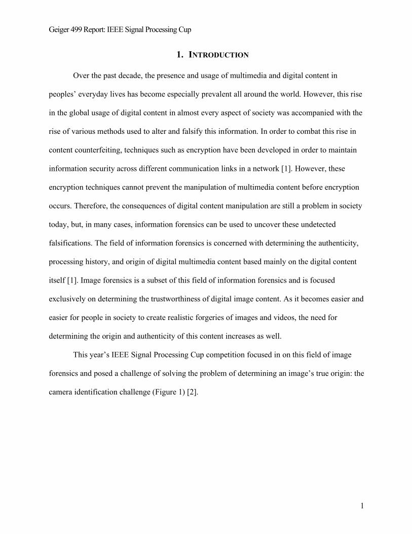
This year’s IEEE Signal Processing Cup competition focused in on this field of image
forensics and posed a challenge of solving the problem of determining an image’s true origin: the
camera identification challenge (Figure 1) [2].
Geiger 499 Report: IEEE Signal Processing Cup
2
FIGURE 1: SOURCE CAMERA IDENTIFICATION CHALLENGE [2]
Information about the type of camera used to capture an image can explicitly provide an answer
to this origin question as well as provide an effective method of applying these classification
methods in several real-world situations. The classification system that teams were required to
build for the Signal Processing Cup competition needed to be able to receive an image as an
input and then use trained machine learning classifiers to determine the make and model of the
camera used to capture that image [2]. The scale on which these classifications systems operated
was limited to a specified range of just ten different camera models, so the application of these
classification systems is slightly restricted as a result. However, the classification methods used
in each system can be directly and effectively applied to more complex systems that are required
to classify more extensive camera model subsets, thus enhancing the applicability of this year’s
Signal Processing Cup competition to the world of information forensics.
The rest of this report is organized as follows: section two will cover an overview of
several techniques that have been applied to solving this camera identification challenge along
with the potential impacts of this identification challenge on various present-day health and
safety, social, political, and ethical issues; section three will cover the detailed design
specifications provided by the 2018 IEEE Signal Processing Cup challenge, the overarching
functional decomposition of the project, and the selection of the design criterion for the final

Geiger 499 Report: IEEE Signal Processing Cup
3
system design; section four will present several different detailed design alternatives and the
reasons behind the final design choice for this project; section five will present the preliminary
proposed design of this project in its entirety with as much detail as possible to conclude the
ECE 498 report; section six will present the final design and implementation of the submitted
classification system to the 2018 IEEE Signal Processing Cup; section seven will present the
performance estimates and results of this final image classification system; section eight will
present the production schedule followed during the Winter Term in order to meet the
competition deadline; section nine will present a cost analysis of this system; section ten will
present a User’s Manual in order to duplicate the overall training and testing of our system; and
section eleven will present a discussion, conclusion, and recommendations

Geiger 499 Report: IEEE Signal Processing Cup
4
2. BACKGROUND INFORMATION
2.1 Camera Identification Context & Previous Work
An essential part of developing a classification system for digital content is developing
unique signatures for each content source. These signatures are constructed through the analysis
of intrinsic fingerprints that are left over in the content itself as a result of different content
processing steps [1]. This allows for not only the ability authenticating content’s origin but also
the ability to trace back the content’s processing history. In respect to the goals of this project,
the unique signatures for each camera model can be developed through inspection and analysis
of a digital camera’s internal processing pipeline (Figure 2).
FIGURE 2: A TYPICAL DIGITAL CAMERA’S INTERNAL PROCESSING PIPELINE [2]
As shown in Figure 2, light enters the camera through a lens, which focuses light on an optical
sensor. This light passes through a color filter array (CFA) that is located between the lens and
the sensor. The CFA is an optical array that only allows for one color-band of light to reach the
sensor at each pixel location. Thus, the image constructed by the optical sensor is missing the
remaining two color-bands at each pixel location and must then interpolate the missing
information. This process of color interpolation is known as demosaicing. After this process, the
image may then be further processed internally through various color balancing and JPEG
compression processes depending on the specific camera [2]. After all of these internal
processes, the output image is produced.

Geiger 499 Report: IEEE Signal Processing Cup
5
As mentioned above, each of these internal processes within the processing pipeline in a
digital camera imprints its unique intrinsic footprint contained within the final output image and
can therefore each be used to develop unique signatures for specific camera models. Research
has been conducted in the past that has used the different fingerprints from a camera’s processing
pipeline to build a classification system that attempts to tackle this camera identification
problem. For example, it is possible to model and estimate the demosaicing filter used by a
camera or to capture pixel dependency values introduced by the demosaicing process by
developing several forensic algorithms [3], [4], [5]. The make and model of an image’s source
camera can be determined using statistical models of sensor noise and other noise sources [6],
[7]. Also, during JPEG compression, traces are left behind by proprietary quantization tables [8].
Additionally, camera model traces can be captured using statistical techniques from steganalysis
[9] and heuristically designed feature sets [10].
Thus, it is possible to construct a “fingerprint” for that camera model with this forensic
information from many images taken from a specific camera model. Several fingerprints are then
constructed for each camera model in question and are used as classification features when
training a machine learning algorithm to recognize an image’s source camera model.
2.2 Potential Impacts on Present-Day Issues
The camera identification challenge has a number of implications on present-day health
and safety, social, political, and ethical issues. First of all, the ability to determine the
authenticity of images can positively impact the health and safety of society. Images are often
used as evidence in criminal investigations, which include investigations regarding blackmail,
child exploitation, homicide, and many others. In each of these cases, it would be essential for
Geiger 499 Report: IEEE Signal Processing Cup
6
the criminal investigators to know if all of the data present shown in an image is authentic and as
well as determining from where these images came with a certain amount of confidence. The
application of these camera identification techniques would be helping to ensure the safety of the
victims involved in these specific criminal cases. On a broader note, the military and defense
agencies of a nation could use these techniques to verify the authenticity and origin of images
used as intel for different scenarios. Consequently, techniques for camera identification would be
helping to either maintain or improve national health and security depending on the nature of the
situation.
The significant presence that the media has in people’s everyday lives makes the effects
of these camera identification techniques especially impactful in a positive way. With the almost
universal availability to image editing and fabricating software, the likelihood of counterfeit
images being spread through the media is relatively high, especially if these images are as
realistic as the originals. This causes the incredibly-persuasive media to sometimes spread fake
news through a huge population of media followers, which could potentially influence the
opinions and reactions of viewers to this false information. The amount of influence that the
media has on the general public substantially increases the need of filtering out this false
information in the form of counterfeit images. This filtering process is where these camera
identification techniques would have the greatest impact and, therefore, help increase the
likelihood of the spread of truthful information to a society.
The spread of counterfeit information through the media to the general public also can
have a direct effect in politics as well. Much of politics relies on elections based on the
popularity of various politicians, so as one can imagine, having a relatively-well-respected
reputation is essential to having a successful political career. Any information that could
Geiger 499 Report: IEEE Signal Processing Cup
7
negatively impact a politician’s reputation would unfairly set that person at a disadvantage
depending on the severity of the information. In order to reduce the spread of this fake news,
such as realistically-fabricated images for example, it would be positively impactful to have
systems in place that could help filter out this information. And, as for the case of filtering out
counterfeit images, implementing these camera identification techniques would be especially
useful.
However, on a more negative side of things, these camera identification techniques could
also present some ethical problems. Camera identification techniques can be used to uncover
similarities between the internal processes of different camera models, thus exposing possible
cases of intellectual property theft [5]. However, if it is possible to expose possible intellectual
property theft using these techniques, then it also must be possible to commit intellectual
property theft using these techniques as well. While the act of committing or attempting to
commit intellectual property theft is a definite ethical crime, the act of watching this event take
place also presents a serious ethical issue. For example, if a camera development engineer
witnesses his coworker or supervisor using camera identification techniques to steal processing
techniques from a rival camera company, then this camera development engineer would be at the
crossroads of a significant ethical dilemma. Either he or she puts his or her job at risk by making
the ethical decision to either speak up against this act or to threaten quitting, or he or she makes
the unethical decision to keep his or her mouth shut and go along with the criminal acts. This is a
very difficult ethical decision for any professional engineer to make, but situations like these
have a chance of coming up during one’s career and he or she must be prepared to do what is
right. Thus, although the general application of these camera identification techniques might not

Geiger 499 Report: IEEE Signal Processing Cup
8
introduce ethical issues, more specified applications of these techniques could unveil some
serious ethical issues.
Geiger 499 Report: IEEE Signal Processing Cup
9
3. DESIGN REQUIREMENTS
The design requirements for this project have been specifically outlined in the 2018
Signal Process Cup competition document provided by the IEEE Signal Processing Society, the
sponsors of this competition [2]. The overall goal of this year’s Signal Processing Cup
competition was to build a system capable of identifying the camera make and model used to
capture a digital image. The competition was comprised of two stages of competition: Open
Competition, which was open to any eligible team of undergraduate students, and Final
Competition, which was open only to the three finalists of the competition.
3.1 Open Competition
The Open Competition was divided into three separate parts for this year’s Signal
Processing Cup: Part 1, Part 2, and the Data Collection Task. The Data Collection Task of Open
Competition will be left out of this report because it required teams to gather 250 images from a
camera not provided in the original dataset and, therefore, has no effect on the overall design of
the classification system that makes up this report. The deliverables for Open Competition were
due February 8, 2018.
3.1.1 Open Competition – Part 1
For Part 1 of Open Competition, teams were provided with a dataset with which to use to
build and train their camera model identification systems. The dataset was comprised of ten
different camera models along with 275 images for each camera model, totaling 2,750 images at
teams’ disposal. In order for teams to evaluate their classifier systems, a new evaluation dataset
was released approximately one month prior to the February 8 submission deadline. This
Geiger 499 Report: IEEE Signal Processing Cup
10
evaluation dataset was comprised of images captured using devices different from those used to
create the training dataset. This required teams to build a camera identification system that
correctly classifies all devices of a particular camera make and model – not to the specific
devices used to capture the images in the training dataset.
3.1.2 Open Competition – Part 2
For Part 2 of Open Competition, teams were required to determine the make and model
of cameras used to capture images that have been post-processed. Examples of image post-
processing include JPEG-recompression, cropping, contrast enhancement, etc. So, for this part of
Open Competition, teams were required to build a camera identification system similar to Part 1
that was fine-tuned to classifying post-processed images. In order to build their classification
systems, teams were provided with a list of all possible post-processing operations that will be
considered along with a Matlab script that can be used to generate post-processed images from
the original dataset of unaltered images (see Appendix A). Upon generating their own post-
processed image dataset, teams then needed to use this as a training dataset with which to build
their camera identification systems. And, again, as in Part 1, teams were provided with an
evaluation dataset approximately one month prior to the February 8 submission deadline.
3.1.3 Open Competition – Deliverables
The following material must be submitted by the February 8, 2018 deadline in order to be
considered for the Final Competition [2]:
1. A report in the form of an IEEE conference paper describing the technical details of the
system.
Geiger 499 Report: IEEE Signal Processing Cup
11
2. Camera model identification results from Open Competition.
3. Data Collection Task.
4. An executable with a Matlab implementation of the camera model identification system.
This should be able to accept an input in the form of a directory of images and produce a
text file identifying the camera model used to capture each image in the directory.
3.2 Final Competition
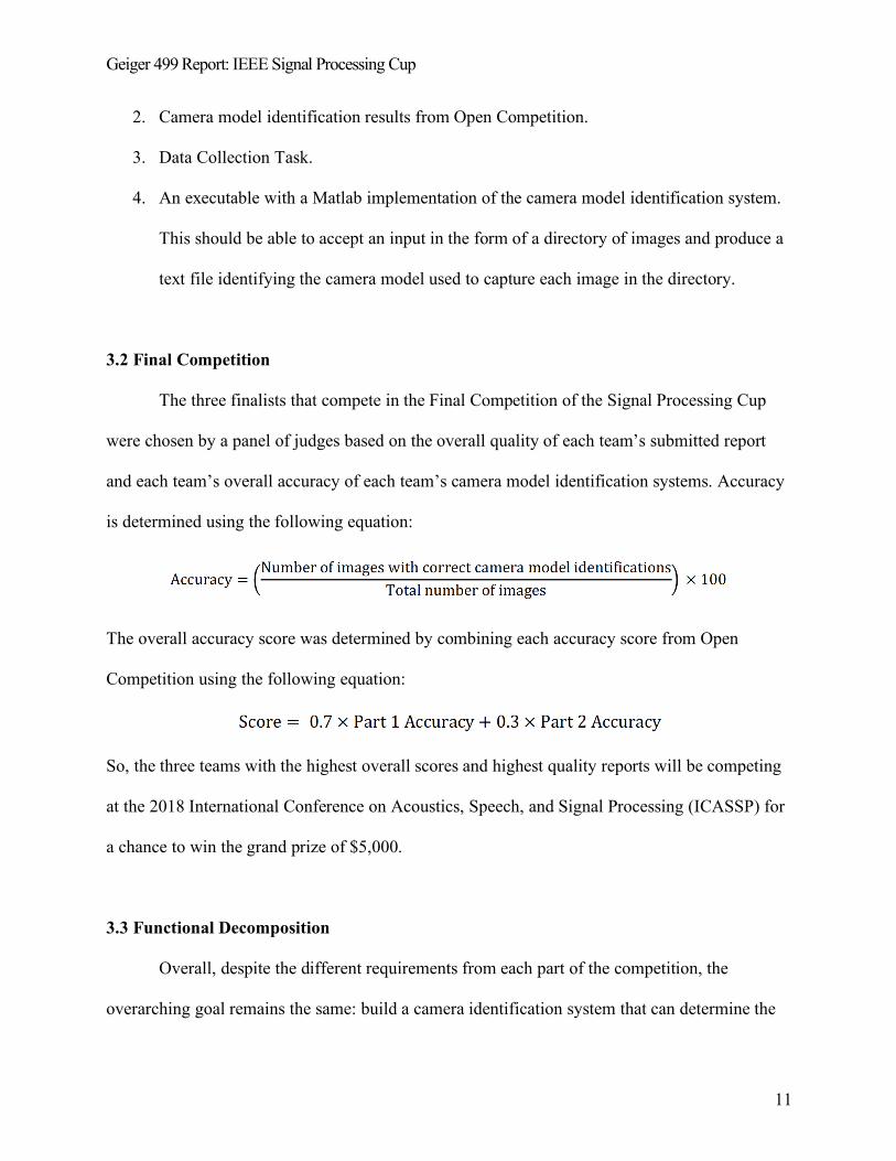
The three finalists that compete in the Final Competition of the Signal Processing Cup
were chosen by a panel of judges based on the overall quality of each team’s submitted report
and each team’s overall accuracy of each team’s camera model identification systems. Accuracy
is determined using the following equation:
The overall accuracy score was determined by combining each accuracy score from Open
Competition using the following equation:
So, the three teams with the highest overall scores and highest quality reports will be competing
at the 2018 International Conference on Acoustics, Speech, and Signal Processing (ICASSP) for
a chance to win the grand prize of $5,000.
3.3 Functional Decomposition
Overall, despite the different requirements from each part of the competition, the
overarching goal remains the same: build a camera identification system that can determine the
Geiger 499 Report: IEEE Signal Processing Cup
12
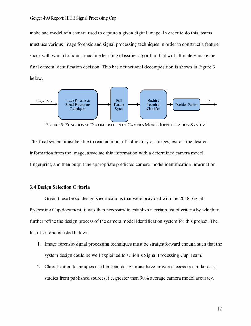
make and model of a camera used to capture a given digital image. In order to do this, teams
must use various image forensic and signal processing techniques in order to construct a feature
space with which to train a machine learning classifier algorithm that will ultimately make the
final camera identification decision. This basic functional decomposition is shown in Figure 3
below.
FIGURE 3: FUNCTIONAL DECOMPOSITION OF CAMERA MODEL IDENTIFICATION SYSTEM
The final system must be able to read an input of a directory of images, extract the desired
information from the image, associate this information with a determined camera model
fingerprint, and then output the appropriate predicted camera model identification information.
3.4 Design Selection Criteria
Given these broad design specifications that were provided with the 2018 Signal
Processing Cup document, it was then necessary to establish a certain list of criteria by which to
further refine the design process of the camera model identification system for this project. The
list of criteria is listed below:
1. Image forensic/signal processing techniques must be straightforward enough such that the
system design could be well explained to Union’s Signal Processing Cup Team.
2. Classification techniques used in final design must have proven success in similar case
studies from published sources, i.e. greater than 90% average camera model accuracy.

Geiger 499 Report: IEEE Signal Processing Cup
13
The first criterion comes in respect to the fact that this project included leading Union’s Signal
Processing Cup Team in this year’s competition. Since Union’s team was comprised of
undergraduate students with varying levels of signal processing experience, the final design
choice must have been intuitive enough that the specific functionality of the design could be
easily explained to all team members. The second criterion establishes a filtering method while
researching possible classification techniques to solve this camera model identification
challenge. This restricts the focus of possible final designs to camera classification systems that
have been implemented with average camera model accuracy of at least 90%. Keeping these
criteria in mind, it was next possible to narrow the possible design selections to a select handful
of possibilities.
Geiger 499 Report: IEEE Signal Processing Cup
14
4. DESIGN ALTERNATIVES
Along with the 2018 IEEE Signal Processing Cup competition document, the IEEE
Signal Processing also provided teams with several supplementary references to learn about the
camera model identification challenge. A majority of these references presented different
methods of solving this challenge, so the goal of this research was to deduce which methods
were going to be the best to implement based on the established design selection criteria in
Section 3.4. The design selection process used deductive reasoning to eliminate some possible
methods from final design contention.
Some possible design alternatives were noise-based methods, which use statistical
models of sensor noise and other noise sources to identify the make and model of an image’s
source camera [2]. The sensor noise model, otherwise known as the photo-response non-
uniformity (PRNU) model, can reliably identify a specific camera, and was proven to do so in
[6]. The other noise model mentioned above is the heteroscedastic noise model, which can be
used to describe a natural raw image [7]. The first issue with these models was the relatively high
likelihood of developing a classifier that over fit the classification of the camera models to each
of the specific devices used to construct the image database. This would result in a classifier that
had almost perfect training accuracy but would perform very poorly when it had to classify
images captured using different devices of the same camera makes and models as provided in the
image database. In addition to this potential design flaw, the statistical models used in both of
these noise-based camera identification models were incredibly dense. This presented the
difficult challenge of being able to understand the models well enough to not only implement
them in our own system but also to be able to easily teach them to the other team members of
Geiger 499 Report: IEEE Signal Processing Cup
15
Union’s Signal Processing Cup team. These two points were key factors in ruling out using a
noise-based classifier system design for this project.
After ruling out a noise-based classifier design, the next best option was a demosaicing-
based classifier. Out of all of the studies provided as references by the IEEE Signal Processing
Society, three of them were studies showing the effectiveness of a demosaicing-based classifier:
two studies attempted to identify specific CFAs and demosaicing algorithms in order to solve
this camera identification challenge, and the third study was the study selected as the basis of
design for this project’s camera model identification system. The first of these studies used
techniques aimed at determining the parameters of CFA and demosaicing algorithms, but
however were only able to achieve an overall accuracy of 90% [3]. The accuracy of this system
was the lowest of the three demosaicing studies presented, so it was then eliminated from final
design contention. The second of these studies aimed at using techniques to identify sixteen
different demosaicing algorithms, with which to then use as a way of identifying a camera’s
make and model to an average overall system accuracy of 98.3% [4]. The only flaw to this
design, which was the eventual reason for elimination from final design contention, was the
relative complexity of the classification methods used. Compared to the final design used in this
project, which is based off of the design used in [5], the overall accuracies of the systems were
almost equal; however, the final design chosen for this project was much more straightforward
and easier to understand than the design used in [4]. Thus, this comparison of designs made the
ultimate decision for the final design for the camera identification system to be based off of the
design used in [4].
Geiger 499 Report: IEEE Signal Processing Cup
16
5. PRELIMINARY PROPOSED DESIGN
The preliminary proposed design for this project is based off of the design of a general
camera identification system design that was explained in [5]. The authors of this paper used a
demosaicing-algorithm-based classifier and were able to obtain an average classification
accuracy of 99.2% for their system. The proposed design for this report’s specific camera model
identification system is outlined below and specifically follows the functional composition
outlined in Figure 3.
5.1 Image Forensic Techniques
The camera model identification system design proposed uses three image forensic
techniques in order to construct a full feature space for the classifier: a Bayer CFA filter,
demosaicing algorithms, and co-occurrence matrices.
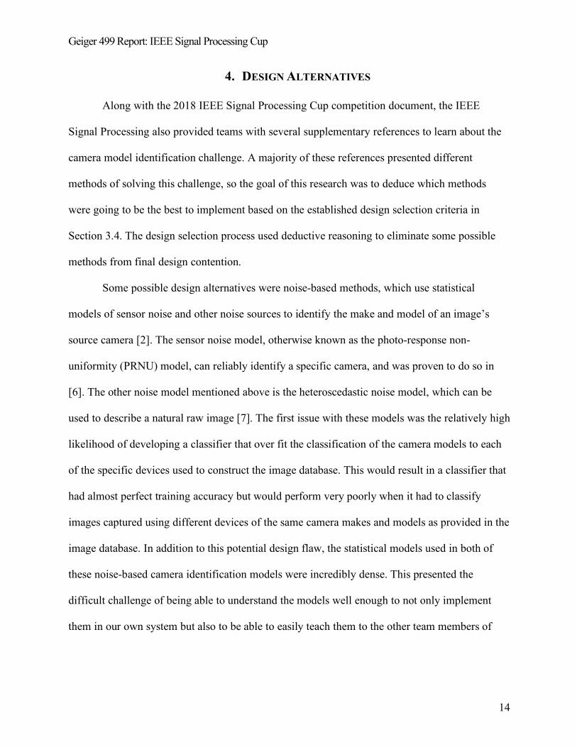
5.1.1 The Bayer CFA Pattern
A color filter array (CFA) is typically a 2x2 repeating pixel pattern that allows only one
color component of light to pass through at each pixel location before the light reaches the sensor
(Figure 4) [2].
FIGURE 4: EXAMPLE CFA PATTERN OPERATION [11]
Geiger 499 Report: IEEE Signal Processing Cup
17
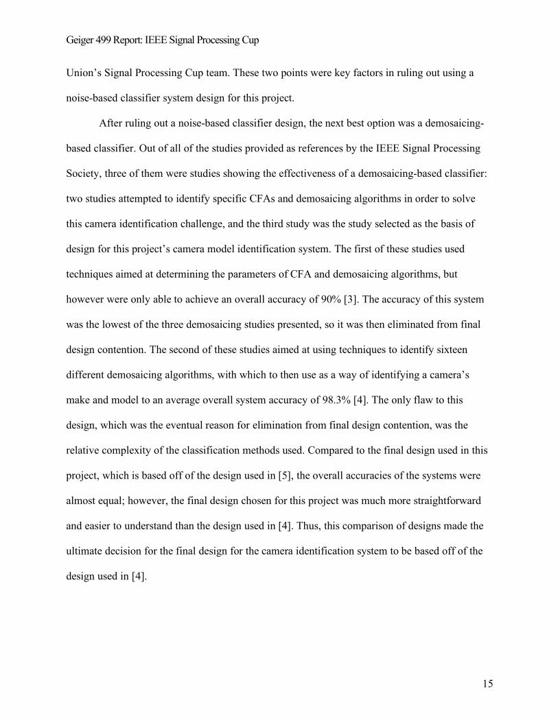
Out of all the CFA patterns, the Bayer pattern (Figure 5) is the most commonly used.
FIGURE 5: THE BAYER CFA PATTERN
The Bayer CFA 2x2 pixel filter pattern can be oriented in four different ways: GBRG (Figure 5),
GRBG (Figure 6), BGGR (Figure 4), and RGGB. As a result of this process, as seen in Figures 4
and 5, the resulting image is missing the remaining two color components at each pixel location,
which requires a process of color interpolation, called demosaicing, to fill in the remaining color
components.
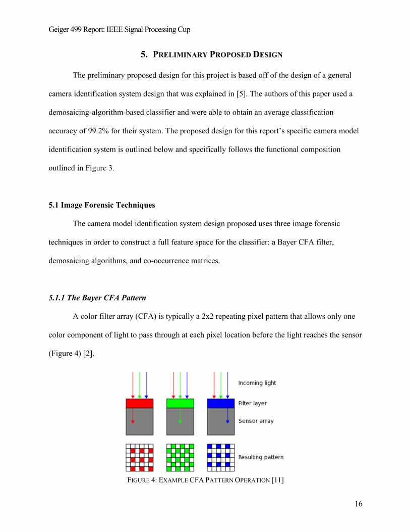
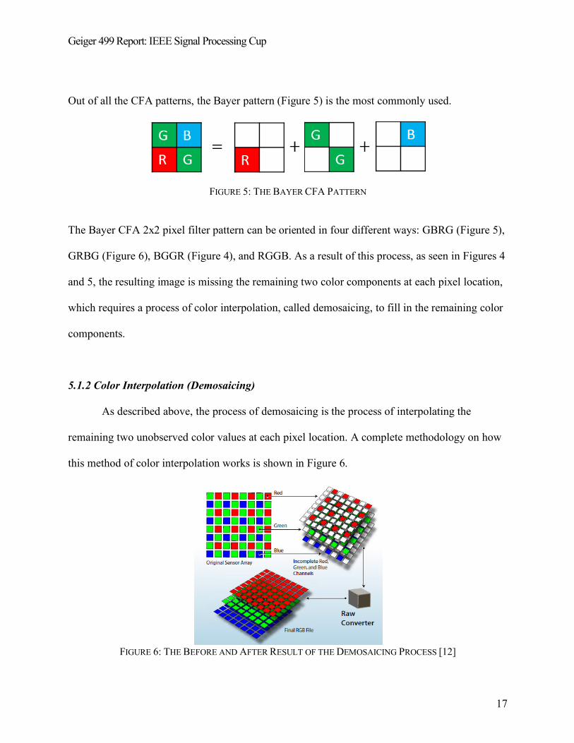
5.1.2 Color Interpolation (Demosaicing)
As described above, the process of demosaicing is the process of interpolating the
remaining two unobserved color values at each pixel location. A complete methodology on how
this method of color interpolation works is shown in Figure 6.
FIGURE 6: THE BEFORE AND AFTER RESULT OF THE DEMOSAICING PROCESS [12]
Geiger 499 Report: IEEE Signal Processing Cup
18
The demosaicing process shown in Figure 6 is the process that occurs at the step which is labeled
“Raw Converter,” which converts this raw image from the sensor into a complete image, i.e. the
demosaicing process. This process is implemented through the use of a demosaicing algorithm.
Some examples of demosaicing algorithms include nearest neighbor interpolation, bilinear
interpolation, and smooth-hue interpolation [13].
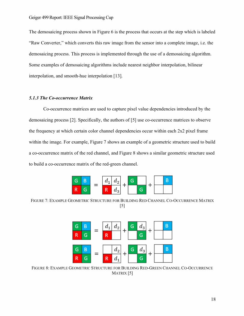
5.1.3 The Co-occurrence Matrix
Co-occurrence matrices are used to capture pixel value dependencies introduced by the
demosaicing process [2]. Specifically, the authors of [5] use co-occurrence matrices to observe
the frequency at which certain color channel dependencies occur within each 2x2 pixel frame
within the image. For example, Figure 7 shows an example of a geometric structure used to build
a co-occurrence matrix of the red channel, and Figure 8 shows a similar geometric structure used
to build a co-occurrence matrix of the red-green channel.
FIGURE 7: EXAMPLE GEOMETRIC STRUCTURE FOR BUILDING RED CHANNEL CO-OCCURRENCE MATRIX
[5]
FIGURE 8: EXAMPLE GEOMETRIC STRUCTURE FOR BUILDING RED-GREEN CHANNEL CO-OCCURRENCE
MATRIX [5]
Geiger 499 Report: IEEE Signal Processing Cup
19
Each of these figures show a single instance of their respective generated co-occurrence matrix
where the values (d1, d2, d3) are compared to their respective locations in each pixel frame. Thus,
these matrices capture pixel value dependencies based on specific color channels of interest.
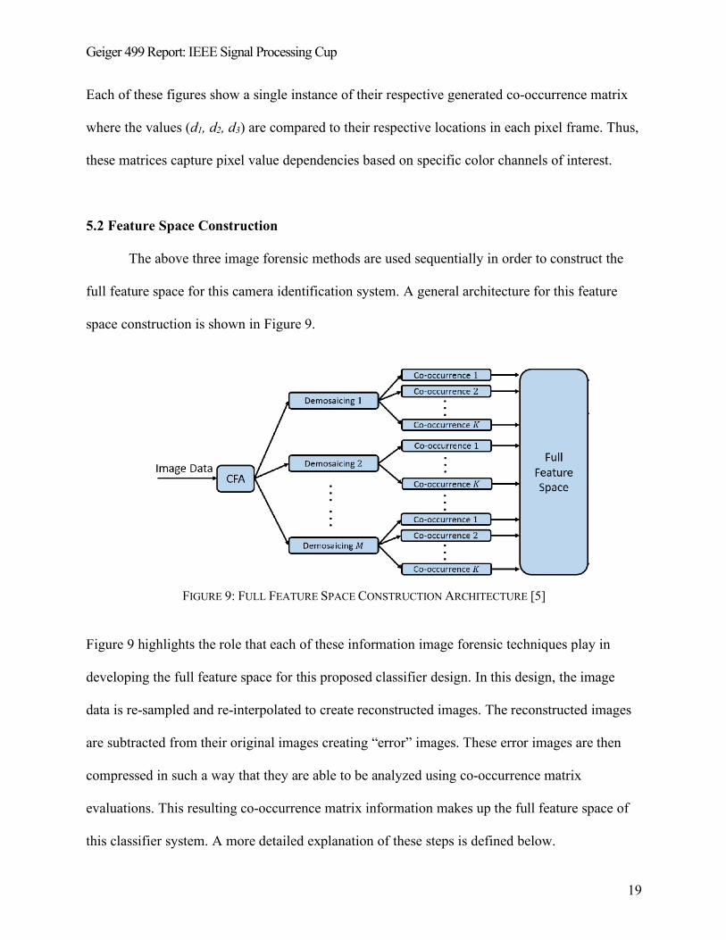
5.2 Feature Space Construction
The above three image forensic methods are used sequentially in order to construct the
full feature space for this camera identification system. A general architecture for this feature
space construction is shown in Figure 9.
FIGURE 9: FULL FEATURE SPACE CONSTRUCTION ARCHITECTURE [5]
Figure 9 highlights the role that each of these information image forensic techniques play in
developing the full feature space for this proposed classifier design. In this design, the image
data is re-sampled and re-interpolated to create reconstructed images. The reconstructed images
are subtracted from their original images creating “error” images. These error images are then
compressed in such a way that they are able to be analyzed using co-occurrence matrix
evaluations. This resulting co-occurrence matrix information makes up the full feature space of
this classifier system. A more detailed explanation of these steps is defined below.
Geiger 499 Report: IEEE Signal Processing Cup
20
5.2.1 Image Re-sampling
The first step towards feature space construction for this proposed design is a re-sampling
of the image data using a CFA pattern. In this proposed design, the specific CFA pattern used is
a Bayer pattern in GBRG format (as seen in Figures 5, 7, and 8). Other Bayer pattern formats can
be used for the re-sampling step, but the GBRG format was chosen because it is the same format
used in [5]. This is important because the co-occurrence matrix calculations provided are very
complex and are based on this specific Bayer pattern format. This allows for an easier
application of the provided co-occurrence matrix calculation equations into this project’s camera
identification system design and implementation.
5.2.2 Image Re-interpolating
The next step of feature space construction is using demosaicing to reconstruct the image
data from the raw image data provided by the CFA filter in the previous step using demosaicing.
At this point in the construction architecture, there are multiple demosaicing algorithms to
choose from here – specifically, there are six algorithms: Nearest Neighbor Interpolation,
Bilinear Interpolation, Smooth Hue Transition Interpolation, Median-Filter Bilinear
Interpolation, Gradient-Based Interpolation, and a Gradient-Corrected Linear Interpolation. Any
combinations of these demosaicing algorithms could be implemented to greatly increase the full
feature space size.
Geiger 499 Report: IEEE Signal Processing Cup
21
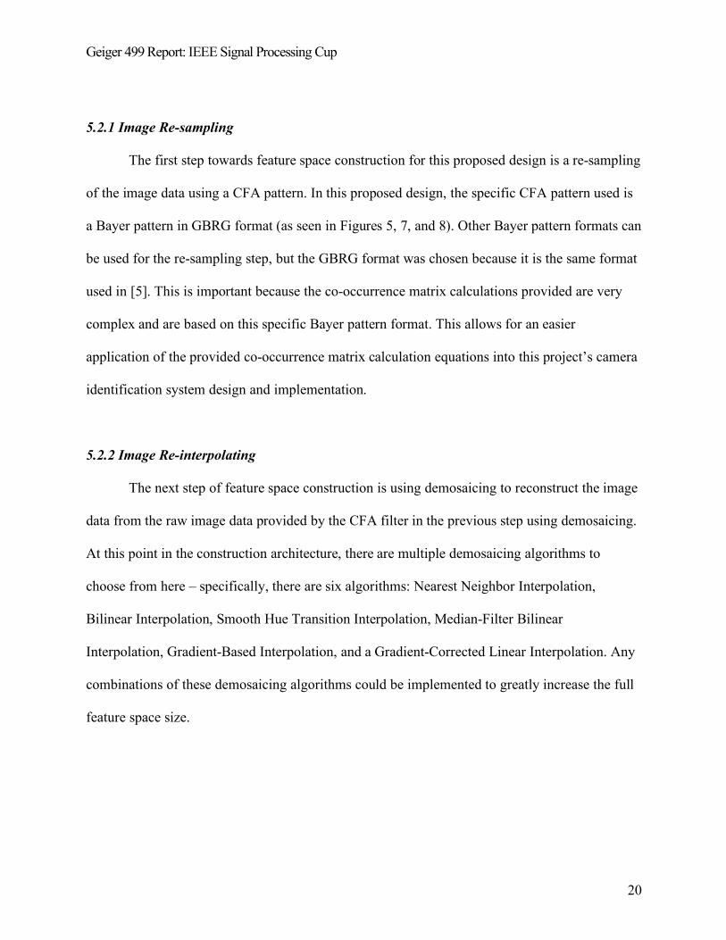
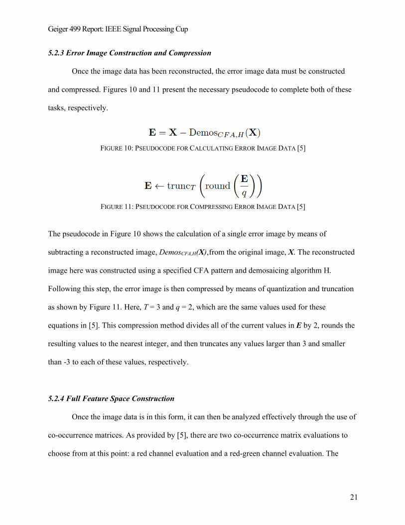
5.2.3 Error Image Construction and Compression
Once the image data has been reconstructed, the error image data must be constructed
and compressed. Figures 10 and 11 present the necessary pseudocode to complete both of these
tasks, respectively.
FIGURE 10: PSEUDOCODE FOR CALCULATING ERROR IMAGE DATA [5]
FIGURE 11: PSEUDOCODE FOR COMPRESSING ERROR IMAGE DATA [5]
The pseudocode in Figure 10 shows the calculation of a single error image by means of
subtracting a reconstructed image, DemosCFA,H(X),from the original image, X. The reconstructed
image here was constructed using a specified CFA pattern and demosaicing algorithm H.
Following this step, the error image is then compressed by means of quantization and truncation
as shown by Figure 11. Here, T = 3 and q = 2, which are the same values used for these
equations in [5]. This compression method divides all of the current values in E by 2, rounds the
resulting values to the nearest integer, and then truncates any values larger than 3 and smaller
than -3 to each of these values, respectively.
5.2.4 Full Feature Space Construction
Once the image data is in this form, it can then be analyzed effectively through the use of
co-occurrence matrices. As provided by [5], there are two co-occurrence matrix evaluations to
choose from at this point: a red channel evaluation and a red-green channel evaluation. The
Geiger 499 Report: IEEE Signal Processing Cup
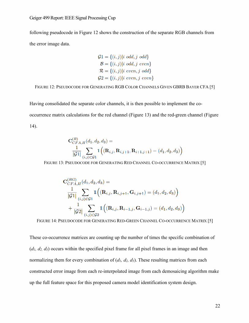
22
following pseudocode in Figure 12 shows the construction of the separate RGB channels from
the error image data.
FIGURE 12: PSEUDOCODE FOR GENERATING RGB COLOR CHANNELS GIVEN GBRB BAYER CFA [5]
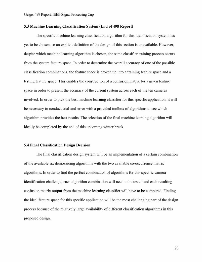
Having consolidated the separate color channels, it is then possible to implement the co-
occurrence matrix calculations for the red channel (Figure 13) and the red-green channel (Figure
14).
FIGURE 13: PSEUDOCODE FOR GENERATING RED CHANNEL CO-OCCURRENCE MATRIX [5]
FIGURE 14: PSEUDOCODE FOR GENERATING RED-GREEN CHANNEL CO-OCCURRENCE MATRIX [5]
These co-occurrence matrices are counting up the number of times the specific combination of
(d1, d2, d3) occurs within the specified pixel frame for all pixel frames in an image and then
normalizing them for every combination of (d1, d2, d3). These resulting matrices from each
constructed error image from each re-interpolated image from each demosaicing algorithm make
up the full feature space for this proposed camera model identification system design.
Geiger 499 Report: IEEE Signal Processing Cup
23
5.3 Machine Learning Classification System (End of 498 Report)
The specific machine learning classification algorithm for this identification system has
yet to be chosen, so an explicit definition of the design of this section is unavailable. However,
despite which machine learning algorithm is chosen, the same classifier training process occurs
from the system feature space. In order to determine the overall accuracy of one of the possible
classification combinations, the feature space is broken up into a training feature space and a
testing feature space. This enables the construction of a confusion matrix for a given feature
space in order to present the accuracy of the current system across each of the ten cameras
involved. In order to pick the best machine learning classifier for this specific application, it will
be necessary to conduct trial-and-error with a provided toolbox of algorithms to see which
algorithm provides the best results. The selection of the final machine learning algorithm will
ideally be completed by the end of this upcoming winter break.
5.4 Final Classification Design Decision
The final classification design system will be an implementation of a certain combination
of the available six demosaicing algorithms with the two available co-occurrence matrix
algorithms. In order to find the perfect combination of algorithms for this specific camera
identification challenge, each algorithm combination will need to be tested and each resulting
confusion matrix output from the machine learning classifier will have to be compared. Finding
the ideal feature space for this specific application will be the most challenging part of the design
process because of the relatively large availability of different classification algorithms in this
proposed design.
Geiger 499 Report: IEEE Signal Processing Cup
24
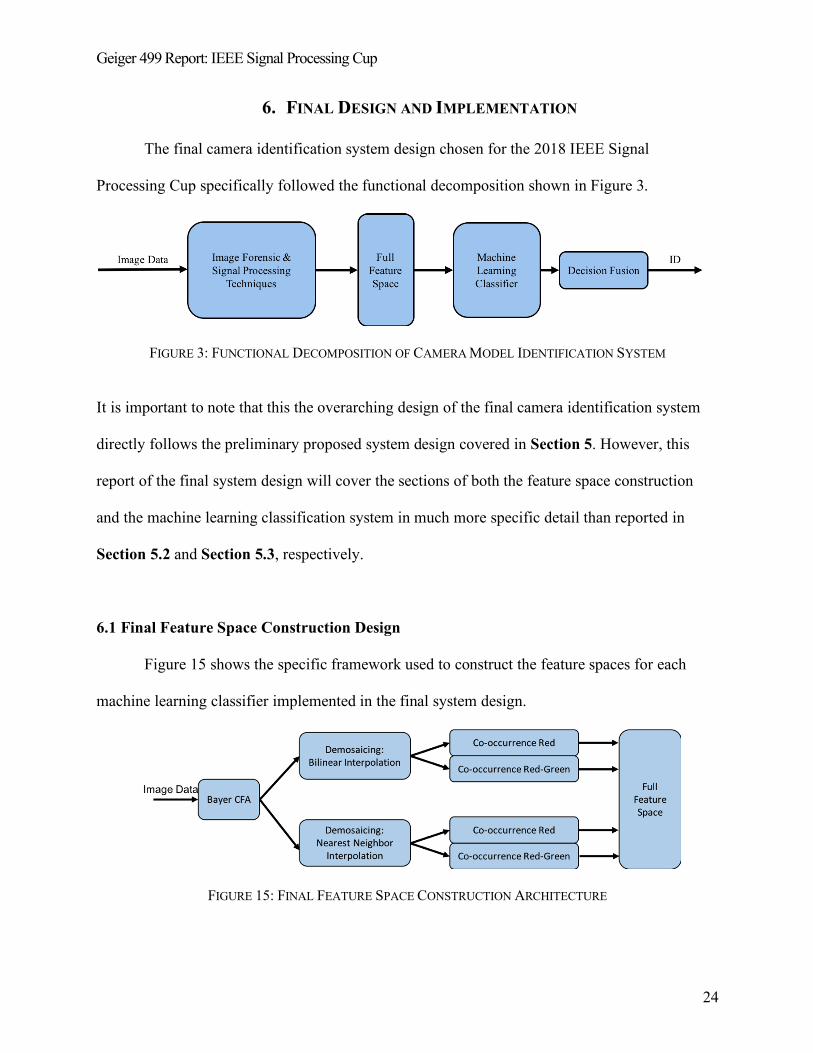
6. FINAL DESIGN AND IMPLEMENTATION
The final camera identification system design chosen for the 2018 IEEE Signal
Processing Cup specifically followed the functional decomposition shown in Figure 3.
FIGURE 3: FUNCTIONAL DECOMPOSITION OF CAMERA MODEL IDENTIFICATION SYSTEM
It is important to note that this the overarching design of the final camera identification system
directly follows the preliminary proposed system design covered in Section 5. However, this
report of the final system design will cover the sections of both the feature space construction
and the machine learning classification system in much more specific detail than reported in
Section 5.2 and Section 5.3, respectively.
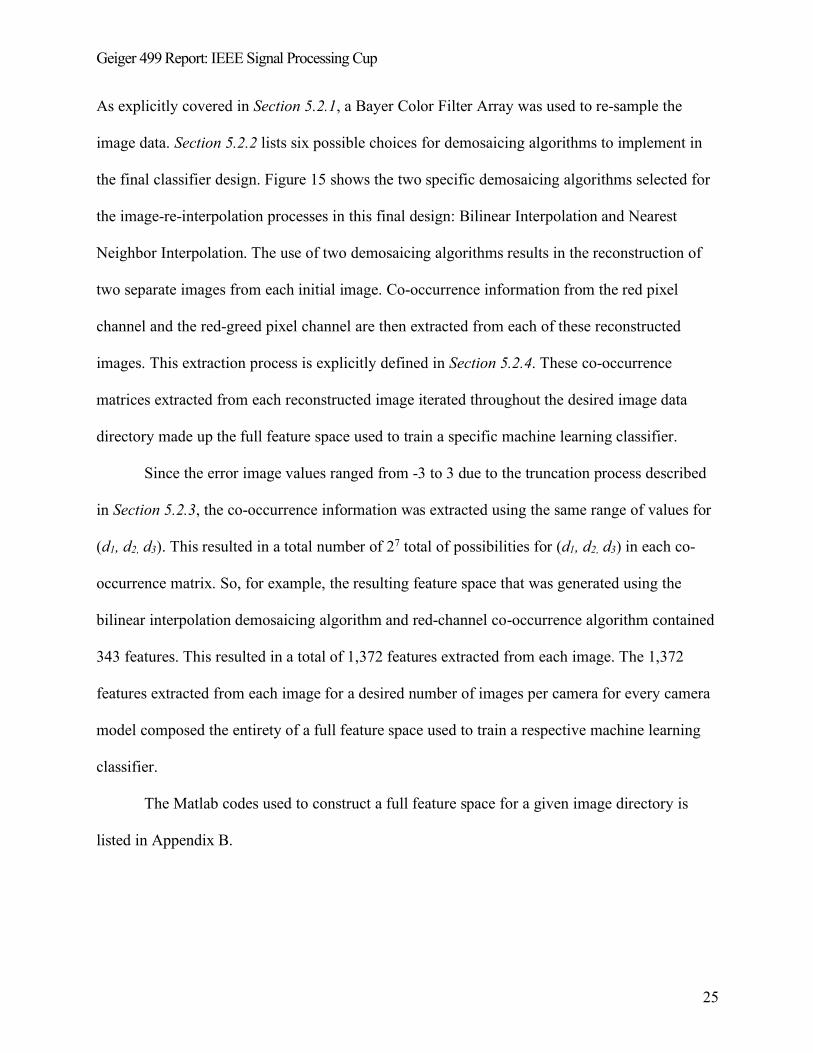
6.1 Final Feature Space Construction Design
Figure 15 shows the specific framework used to construct the feature spaces for each
machine learning classifier implemented in the final system design.
FIGURE 15: FINAL FEATURE SPACE CONSTRUCTION ARCHITECTURE
Geiger 499 Report: IEEE Signal Processing Cup
25
As explicitly covered in Section 5.2.1, a Bayer Color Filter Array was used to re-sample the
image data. Section 5.2.2 lists six possible choices for demosaicing algorithms to implement in
the final classifier design. Figure 15 shows the two specific demosaicing algorithms selected for
the image-re-interpolation processes in this final design: Bilinear Interpolation and Nearest
Neighbor Interpolation. The use of two demosaicing algorithms results in the reconstruction of
two separate images from each initial image. Co-occurrence information from the red pixel
channel and the red-greed pixel channel are then extracted from each of these reconstructed
images. This extraction process is explicitly defined in Section 5.2.4. These co-occurrence
matrices extracted from each reconstructed image iterated throughout the desired image data
directory made up the full feature space used to train a specific machine learning classifier.
Since the error image values ranged from -3 to 3 due to the truncation process described
in Section 5.2.3, the co-occurrence information was extracted using the same range of values for
(d1, d2, d3). This resulted in a total number of 27 total of possibilities for (d1, d2, d3) in each co-
occurrence matrix. So, for example, the resulting feature space that was generated using the
bilinear interpolation demosaicing algorithm and red-channel co-occurrence algorithm contained
343 features. This resulted in a total of 1,372 features extracted from each image. The 1,372
features extracted from each image for a desired number of images per camera for every camera
model composed the entirety of a full feature space used to train a respective machine learning
classifier.
The Matlab codes used to construct a full feature space for a given image directory is
listed in Appendix B.
Geiger 499 Report: IEEE Signal Processing Cup
26
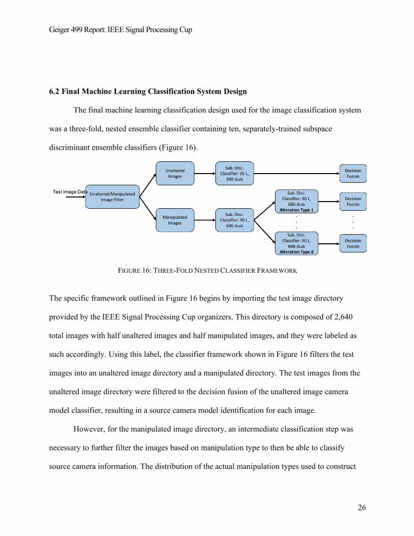
6.2 Final Machine Learning Classification System Design
The final machine learning classification design used for the image classification system
was a three-fold, nested ensemble classifier containing ten, separately-trained subspace
discriminant ensemble classifiers (Figure 16).
FIGURE 16: THREE-FOLD NESTED CLASSIFIER FRAMEWORK
The specific framework outlined in Figure 16 begins by importing the test image directory
provided by the IEEE Signal Processing Cup organizers. This directory is composed of 2,640
total images with half unaltered images and half manipulated images, and they were labeled as
such accordingly. Using this label, the classifier framework shown in Figure 16 filters the test
images into an unaltered image directory and a manipulated directory. The test images from the
unaltered image directory were filtered to the decision fusion of the unaltered image camera
model classifier, resulting in a source camera model identification for each image.
However, for the manipulated image directory, an intermediate classification step was
necessary to further filter the images based on manipulation type to then be able to classify
source camera information. The distribution of the actual manipulation types used to construct
Geiger 499 Report: IEEE Signal Processing Cup
27
the 1320 manipulated images was not provided, so this intermediate classification step was used
to determine the specific technique used to manipulate each image in this filtered directory.
Since there were eight possible manipulation techniques (as shown in Appendix A), there were
eight camera model classifiers trained to determine the camera make and model of each image.
Therefore, the test images from the manipulated image directory were first filtered to the
decision fusion of the manipulation type classifier, resulting in a manipulation type identification
for each image. From here, these images were then filtered to their respective manipulation type
camera model classifier, resulting in a source camera model identification for each image.
6.2.1 Subspace Discriminant Ensemble Classifier Training Information
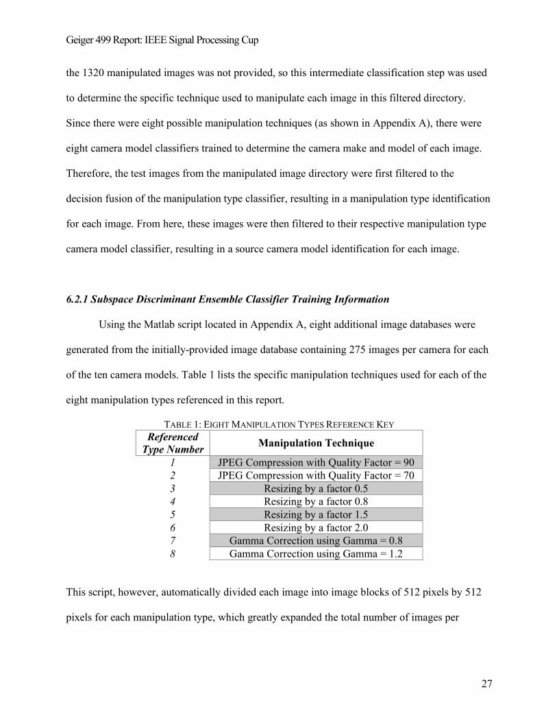
Using the Matlab script located in Appendix A, eight additional image databases were
generated from the initially-provided image database containing 275 images per camera for each
of the ten camera models. Table 1 lists the specific manipulation techniques used for each of the
eight manipulation types referenced in this report.
TABLE 1: EIGHT MANIPULATION TYPES REFERENCE KEY Referenced
Type Number Manipulation Technique
1 JPEG Compression with Quality Factor = 90 2 JPEG Compression with Quality Factor = 70 3 Resizing by a factor 0.5 4 Resizing by a factor 0.8 5 Resizing by a factor 1.5 6 Resizing by a factor 2.0 7 Gamma Correction using Gamma = 0.8 8 Gamma Correction using Gamma = 1.2
This script, however, automatically divided each image into image blocks of 512 pixels by 512
pixels for each manipulation type, which greatly expanded the total number of images per
Geiger 499 Report: IEEE Signal Processing Cup
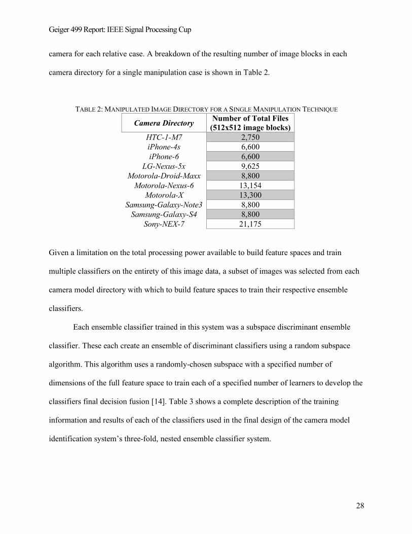
28
camera for each relative case. A breakdown of the resulting number of image blocks in each
camera directory for a single manipulation case is shown in Table 2.
TABLE 2: MANIPULATED IMAGE DIRECTORY FOR A SINGLE MANIPULATION TECHNIQUE
Camera Directory Number of Total Files (512x512 image blocks)
HTC-1-M7 2,750 iPhone-4s 6,600 iPhone-6 6,600
LG-Nexus-5x 9,625 Motorola-Droid-Maxx 8,800
Motorola-Nexus-6 13,154 Motorola-X 13,300
Samsung-Galaxy-Note3 8,800 Samsung-Galaxy-S4 8,800
Sony-NEX-7 21,175
Given a limitation on the total processing power available to build feature spaces and train
multiple classifiers on the entirety of this image data, a subset of images was selected from each
camera model directory with which to build feature spaces to train their respective ensemble
classifiers.
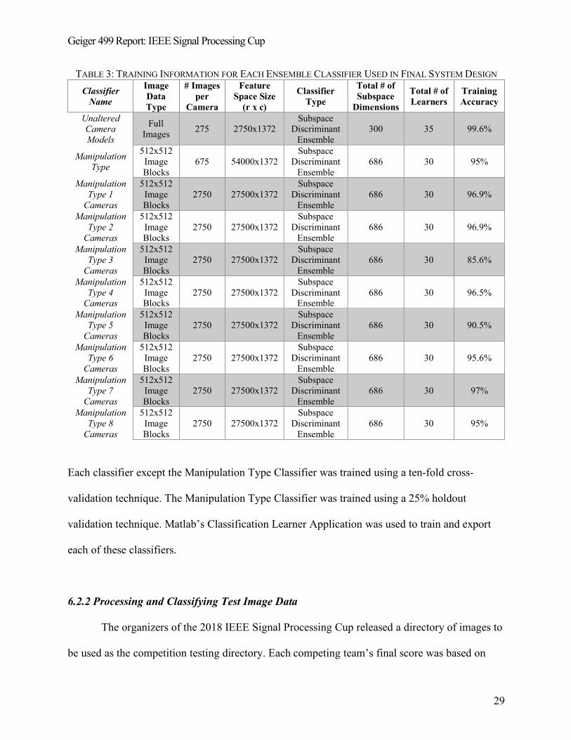
Each ensemble classifier trained in this system was a subspace discriminant ensemble
classifier. These each create an ensemble of discriminant classifiers using a random subspace
algorithm. This algorithm uses a randomly-chosen subspace with a specified number of
dimensions of the full feature space to train each of a specified number of learners to develop the
classifiers final decision fusion [14]. Table 3 shows a complete description of the training
information and results of each of the classifiers used in the final design of the camera model
identification system’s three-fold, nested ensemble classifier system.
Geiger 499 Report: IEEE Signal Processing Cup
29
TABLE 3: TRAINING INFORMATION FOR EACH ENSEMBLE CLASSIFIER USED IN FINAL SYSTEM DESIGN Classifier
Name
Image Data Type
# Images per
Camera
Feature Space Size
(r x c)
Classifier Type
Total # of Subspace
Dimensions
Total # of Learners
Training Accuracy
Unaltered Camera Models
Full Images 275 2750x1372
Subspace Discriminant
Ensemble 300 35 99.6%
Manipulation Type
512x512 Image Blocks
675 54000x1372 Subspace
Discriminant Ensemble
686 30 95%
Manipulation Type 1
Cameras
512x512 Image Blocks
2750 27500x1372 Subspace
Discriminant Ensemble
686 30 96.9%
Manipulation Type 2
Cameras
512x512 Image Blocks
2750 27500x1372 Subspace
Discriminant Ensemble
686 30 96.9%
Manipulation Type 3
Cameras
512x512 Image Blocks
2750 27500x1372 Subspace
Discriminant Ensemble
686 30 85.6%
Manipulation Type 4
Cameras
512x512 Image Blocks
2750 27500x1372 Subspace
Discriminant Ensemble
686 30 96.5%
Manipulation Type 5
Cameras
512x512 Image Blocks
2750 27500x1372 Subspace
Discriminant Ensemble
686 30 90.5%
Manipulation Type 6
Cameras
512x512 Image Blocks
2750 27500x1372 Subspace
Discriminant Ensemble
686 30 95.6%
Manipulation Type 7
Cameras
512x512 Image Blocks
2750 27500x1372 Subspace
Discriminant Ensemble
686 30 97%
Manipulation Type 8
Cameras
512x512 Image Blocks
2750 27500x1372 Subspace
Discriminant Ensemble
686 30 95%
Each classifier except the Manipulation Type Classifier was trained using a ten-fold cross-
validation technique. The Manipulation Type Classifier was trained using a 25% holdout
validation technique. Matlab’s Classification Learner Application was used to train and export
each of these classifiers.
6.2.2 Processing and Classifying Test Image Data
The organizers of the 2018 IEEE Signal Processing Cup released a directory of images to
be used as the competition testing directory. Each competing team’s final score was based on
Geiger 499 Report: IEEE Signal Processing Cup
30
their overall camera model classification accuracy of each image in this directory. As mentioned
above in Section 6.2, this directory was composed of 2,640 total images, half of which were
manipulated in some undisclosed way. In order to apply the trained, machine-learning decision
fusions to this test image data, a feature space of this data must first have been extracted using
the exact same techniques used to construct the training feature spaces from the provided image
directories (Matlab scripts located in Appendix B). Once this test feature space had been
constructed, it could then be filtered through the designed nested ensemble classifier containing
each of the ten, trained decision fusions to predict the source camera information for each test
image. The Matlab script used to implement this nested ensemble classifier is located in
Appendix C.
Geiger 499 Report: IEEE Signal Processing Cup
31
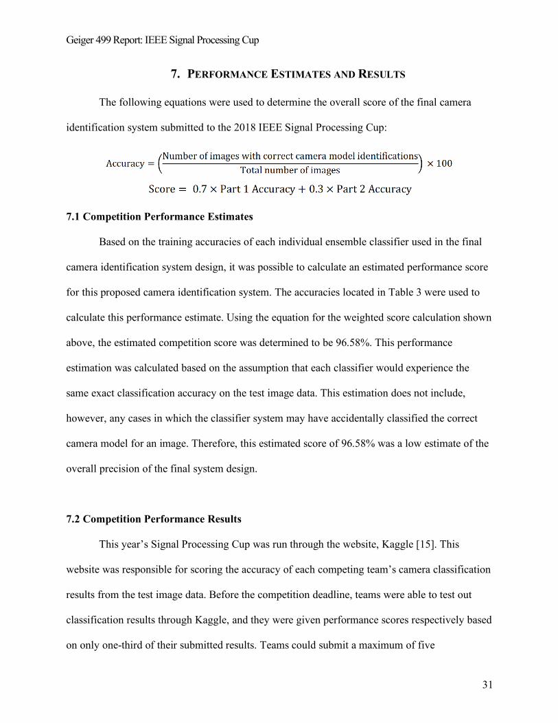
7. PERFORMANCE ESTIMATES AND RESULTS
The following equations were used to determine the overall score of the final camera
identification system submitted to the 2018 IEEE Signal Processing Cup:
7.1 Competition Performance Estimates
Based on the training accuracies of each individual ensemble classifier used in the final
camera identification system design, it was possible to calculate an estimated performance score
for this proposed camera identification system. The accuracies located in Table 3 were used to
calculate this performance estimate. Using the equation for the weighted score calculation shown
above, the estimated competition score was determined to be 96.58%. This performance
estimation was calculated based on the assumption that each classifier would experience the
same exact classification accuracy on the test image data. This estimation does not include,
however, any cases in which the classifier system may have accidentally classified the correct
camera model for an image. Therefore, this estimated score of 96.58% was a low estimate of the
overall precision of the final system design.
7.2 Competition Performance Results
This year’s Signal Processing Cup was run through the website, Kaggle [15]. This
website was responsible for scoring the accuracy of each competing team’s camera classification
results from the test image data. Before the competition deadline, teams were able to test out
classification results through Kaggle, and they were given performance scores respectively based
on only one-third of their submitted results. Teams could submit a maximum of five
Geiger 499 Report: IEEE Signal Processing Cup
32
classification submissions every twenty-four hours throughout the entirety of the competition.
However, teams were only allowed to submit two classification attempts for final scoring. The
best final performance results of the camera identification system design proposed in this report
were 65.6% and 65.0%. The classification results that scored higher were generated using the
exact system outlined in Section 6. The classification that was used to generate the lower-scoring
results was using a Manipulation Type Classifier trained on only 300 images per camera instead
of the 675 images per camera used to train the final system design.
7.3 Discussion of Results
The main point of discussion in this section is the 31% discrepancy between the actual
performance score of 65.6% and the predicted performance score of roughly 96.6%. The most
glaring reason behind this drastic difference in performance scores most likely comes from the
problem of overfitting the model to the training data. Since this system is attempting to use, at
most, 1,372 features to develop specific signatures for each of the camera models used to create
the training database, there is a high possibility that the trained systems had developed decision
fusions specifically tuned for the specific devices used to construct the training database. This
would be a significant issue because the cameras used to construct the test image database were
entirely different devices than those used to construct the training image database, hence the
substantial decrease in system accuracy seen here.
Unfortunately, the organizers of this year’s Signal Processing Cup have not yet released
the results of the camera model identification challenge at the time of this report. As a result, it is
almost impossible to understand explicitly how the final classification score of this system was
determined based on the test image data provided. However, in an attempt to further understand
Geiger 499 Report: IEEE Signal Processing Cup
33
the overall performance of this classification system, a mock image database was constructed to
replicate the test image database provided in the Signal Processing Cup competition. This mock
image database was constructed using images from Flickr, an online image database. This
reconstructed test database contained 2,640 images, half of which were unaltered, and half of
which were manipulated using an even distribution of each of the eight manipulation techniques
provided. There was also an even distribution of each of the ten camera models throughout the
unaltered images and throughout each of the manipulation techniques. This provided for the
ability to analyze the overall performance of this camera identification system including the
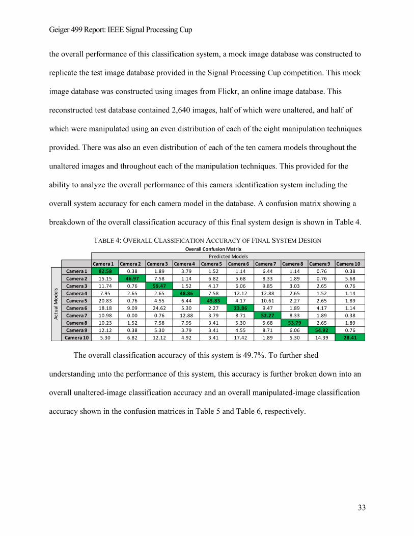
overall system accuracy for each camera model in the database. A confusion matrix showing a
breakdown of the overall classification accuracy of this final system design is shown in Table 4.
TABLE 4: OVERALL CLASSIFICATION ACCURACY OF FINAL SYSTEM DESIGN
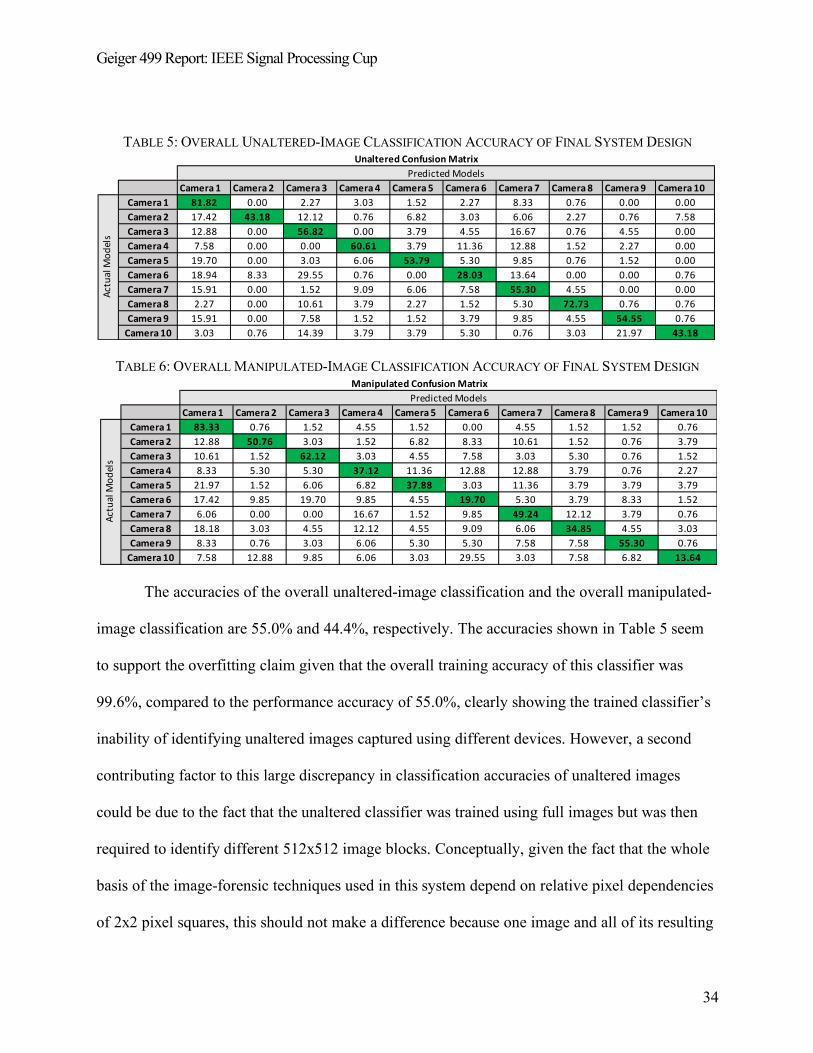
The overall classification accuracy of this system is 49.7%. To further shed
understanding unto the performance of this system, this accuracy is further broken down into an
overall unaltered-image classification accuracy and an overall manipulated-image classification
accuracy shown in the confusion matrices in Table 5 and Table 6, respectively.
Camera 1 Camera 2 Camera 3 Camera 4 Camera 5 Camera 6 Camera 7 Camera 8 Camera 9 Camera 10Camera 1 82.58 0.38 1.89 3.79 1.52 1.14 6.44 1.14 0.76 0.38Camera 2 15.15 46.97 7.58 1.14 6.82 5.68 8.33 1.89 0.76 5.68Camera 3 11.74 0.76 59.47 1.52 4.17 6.06 9.85 3.03 2.65 0.76Camera 4 7.95 2.65 2.65 48.86 7.58 12.12 12.88 2.65 1.52 1.14Camera 5 20.83 0.76 4.55 6.44 45.83 4.17 10.61 2.27 2.65 1.89Camera 6 18.18 9.09 24.62 5.30 2.27 23.86 9.47 1.89 4.17 1.14Camera 7 10.98 0.00 0.76 12.88 3.79 8.71 52.27 8.33 1.89 0.38Camera 8 10.23 1.52 7.58 7.95 3.41 5.30 5.68 53.79 2.65 1.89Camera 9 12.12 0.38 5.30 3.79 3.41 4.55 8.71 6.06 54.92 0.76
Camera 10 5.30 6.82 12.12 4.92 3.41 17.42 1.89 5.30 14.39 28.41
Overall Confusion MatrixPredicted Models
Actu
al M
odel
s
Geiger 499 Report: IEEE Signal Processing Cup
34
TABLE 5: OVERALL UNALTERED-IMAGE CLASSIFICATION ACCURACY OF FINAL SYSTEM DESIGN
TABLE 6: OVERALL MANIPULATED-IMAGE CLASSIFICATION ACCURACY OF FINAL SYSTEM DESIGN
The accuracies of the overall unaltered-image classification and the overall manipulated-
image classification are 55.0% and 44.4%, respectively. The accuracies shown in Table 5 seem
to support the overfitting claim given that the overall training accuracy of this classifier was
99.6%, compared to the performance accuracy of 55.0%, clearly showing the trained classifier’s
inability of identifying unaltered images captured using different devices. However, a second
contributing factor to this large discrepancy in classification accuracies of unaltered images
could be due to the fact that the unaltered classifier was trained using full images but was then
required to identify different 512x512 image blocks. Conceptually, given the fact that the whole
basis of the image-forensic techniques used in this system depend on relative pixel dependencies
of 2x2 pixel squares, this should not make a difference because one image and all of its resulting
Camera 1 Camera 2 Camera 3 Camera 4 Camera 5 Camera 6 Camera 7 Camera 8 Camera 9 Camera 10Camera 1 81.82 0.00 2.27 3.03 1.52 2.27 8.33 0.76 0.00 0.00Camera 2 17.42 43.18 12.12 0.76 6.82 3.03 6.06 2.27 0.76 7.58Camera 3 12.88 0.00 56.82 0.00 3.79 4.55 16.67 0.76 4.55 0.00Camera 4 7.58 0.00 0.00 60.61 3.79 11.36 12.88 1.52 2.27 0.00Camera 5 19.70 0.00 3.03 6.06 53.79 5.30 9.85 0.76 1.52 0.00Camera 6 18.94 8.33 29.55 0.76 0.00 28.03 13.64 0.00 0.00 0.76Camera 7 15.91 0.00 1.52 9.09 6.06 7.58 55.30 4.55 0.00 0.00Camera 8 2.27 0.00 10.61 3.79 2.27 1.52 5.30 72.73 0.76 0.76Camera 9 15.91 0.00 7.58 1.52 1.52 3.79 9.85 4.55 54.55 0.76
Camera 10 3.03 0.76 14.39 3.79 3.79 5.30 0.76 3.03 21.97 43.18
Unaltered Confusion Matrix
Actu
al M
odel
s
Predicted Models
Camera 1 Camera 2 Camera 3 Camera 4 Camera 5 Camera 6 Camera 7 Camera 8 Camera 9 Camera 10Camera 1 83.33 0.76 1.52 4.55 1.52 0.00 4.55 1.52 1.52 0.76Camera 2 12.88 50.76 3.03 1.52 6.82 8.33 10.61 1.52 0.76 3.79Camera 3 10.61 1.52 62.12 3.03 4.55 7.58 3.03 5.30 0.76 1.52Camera 4 8.33 5.30 5.30 37.12 11.36 12.88 12.88 3.79 0.76 2.27Camera 5 21.97 1.52 6.06 6.82 37.88 3.03 11.36 3.79 3.79 3.79Camera 6 17.42 9.85 19.70 9.85 4.55 19.70 5.30 3.79 8.33 1.52Camera 7 6.06 0.00 0.00 16.67 1.52 9.85 49.24 12.12 3.79 0.76Camera 8 18.18 3.03 4.55 12.12 4.55 9.09 6.06 34.85 4.55 3.03Camera 9 8.33 0.76 3.03 6.06 5.30 5.30 7.58 7.58 55.30 0.76
Camera 10 7.58 12.88 9.85 6.06 3.03 29.55 3.03 7.58 6.82 13.64
Manipulated Confusion MatrixPredicted Models
Actu
al M
odel
s
Geiger 499 Report: IEEE Signal Processing Cup
35
512x512 image blocks hold the same amount of information. This claim is supported through the
difference of unaltered and manipulated accuracies of Cameras 4, 5, 6, 7, 8, and 10. In each case,
the overall camera classification accuracy decreases, which could be due to the fact that these
camera classifiers were trained on no more than between 20% and 31% of the total image
information for each camera model directory. However, the increase in overall camera
classification accuracy for Cameras 2, 3, and 9 does not support this claim, making a definitive
claim to explain the phenomena observed here difficult.
This information discussion seems to be further debunked slightly because of how the
accuracy for Camera 1 increases for the manipulated-image case – an increase from 81.82% to
83.33%. In both cases, the entire image directory for Camera 1 was used in the training of each
classifier, but the manipulated-image case had been trained using the manipulated 512x512
image blocks instead. So, this information-dependence seems to only support the phenomena
seen for six out of the ten camera models used for this system.
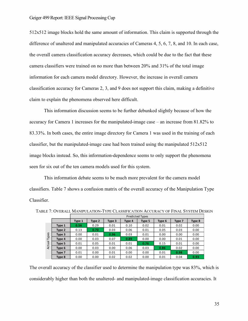
This information debate seems to be much more prevalent for the camera model
classifiers. Table 7 shows a confusion matrix of the overall accuracy of the Manipulation Type
Classifier.
TABLE 7: OVERALL MANIPULATION-TYPE CLASSIFICATION ACCURACY OF FINAL SYSTEM DESIGN
The overall accuracy of the classifier used to determine the manipulation type was 83%, which is
considerably higher than both the unaltered- and manipulated-image classification accuracies. It
Type 1 Type 2 Type 3 Type 4 Type 5 Type 6 Type 7 Type 8Type 1 0.56 0.29 0.01 0.10 0.02 0.01 0.02 0.00Type 2 0.13 0.70 0.03 0.06 0.01 0.05 0.03 0.00Type 3 0.00 0.01 0.96 0.03 0.01 0.00 0.00 0.00Type 4 0.00 0.03 0.07 0.89 0.00 0.00 0.01 0.00Type 5 0.01 0.05 0.01 0.01 0.76 0.15 0.01 0.00Type 6 0.00 0.03 0.00 0.06 0.03 0.86 0.02 0.00Type 7 0.01 0.00 0.01 0.00 0.00 0.01 0.98 0.00Type 8 0.00 0.00 0.02 0.02 0.00 0.01 0.04 0.93
Actu
al Ty
pes
Predicted Types
Geiger 499 Report: IEEE Signal Processing Cup
36
is important to note that this specific classifier was trained using only 675 images per camera
model for each manipulation-type camera directory, resulting in only 6.8% of the entire image
directory from which it was sampled. Despite being trained on a very small percentage of the
entire image directory, it is clear that this specific ensemble classifier was able to much more
effectively predict the manipulation technique used on a processed image than this same
classifier type was able to predict an images camera source. However, this specific classifier was
still not perfect because the estimated accuracy of the Manipulation Type Classifier was 95% (as
listed in Table 3), which is also a significant drop in classification accuracy that should not go
unnoticed. (The Matlab script located in Appendix D was used to generate these confusion
matrices based on the reconstructed test-image database.)
7.4 Suggestions for Improvement
Continuing with this same design, the first and foremost problem to tackle is the
information theory debate. A solution to this problem would be to construct full feature spaces
using the entire directory of 512x512 image blocks for each respective classifier in this system’s
three-fold, nested ensemble design. This would require an immense amount of processing power
because there are 1,372 features being extracted from each image file, and the number of files in
each manipulation-type directory, including unaltered image blocks, increases from 2,750 total
images to 99,604 total images per directory. This would result in feature spaces of dimensions
99604x1372 for the camera model classifiers and then 796,832x1372 for the manipulation type
classifier. After constructing each of these feature spaces, the respective machine learning
classifiers must then be trained accordingly, which would require an immense amount of
processing power for Matlab do build classifiers using matrices containing from around 1.37 x
Geiger 499 Report: IEEE Signal Processing Cup
37
108 elements to around 1.1 x 10⁹ elements. Unfortunately, Union does not have the types of
resources containing the necessary level of computing power, so training this proposed final
system design on the entire information available is not a feasible option.
A loophole around this processing power issue would be to reduce the total number of
features that are extracted from each image file. If it were possible to reduce the total number of
features from 1,372 to less than 100, or even 10, for example, the size of these feature spaces
would drastically reduce, allowing for much more information to be processed using the
resources Union has to offer. The following section uses a method of feature-space-reduction to
observe the resulting changes in overall accuracy of a new unaltered-image classifier derived
from the full feature space used to train the unaltered-image classifier used in this system’s final
design.
7.4.1 Feature Space Reduction of Unaltered-Image Feature Space using Weka
A data mining software, known as Weka, was used to reduce the number of features used
to train the unaltered-image classifier used in this system’s final design. Weka is an open-source,
machine learning software that contains tools for data pre-processing, classification, regression,
clustering, association rules, and visualization [16]. Weka’s Attribute Selector tool was used to
identify the most influential features in the unaltered image feature space constructed using the
full-image database. The specific attribute evaluator algorithm used was the
“ClassifierAttributeEval” (using the default settings), and the search method algorithm used was
the “Ranker” algorithm, which listed a specified number of features from most influential to least
influential. Table 8 shows the resulting training accuracies of two different classifiers that were
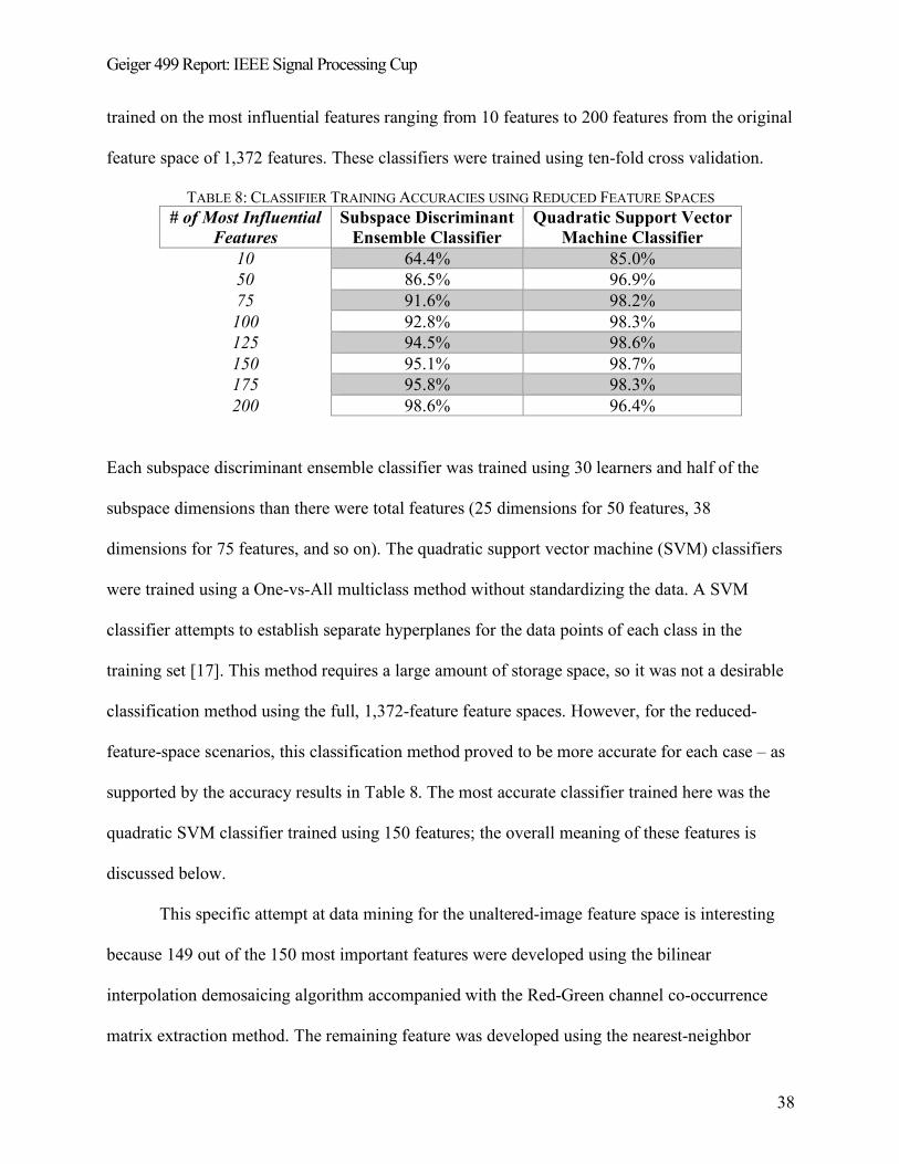
Geiger 499 Report: IEEE Signal Processing Cup
38
trained on the most influential features ranging from 10 features to 200 features from the original
feature space of 1,372 features. These classifiers were trained using ten-fold cross validation.
TABLE 8: CLASSIFIER TRAINING ACCURACIES USING REDUCED FEATURE SPACES # of Most Influential
Features Subspace Discriminant
Ensemble Classifier Quadratic Support Vector
Machine Classifier 10 64.4% 85.0% 50 86.5% 96.9% 75 91.6% 98.2% 100 92.8% 98.3% 125 94.5% 98.6% 150 95.1% 98.7% 175 95.8% 98.3% 200 98.6% 96.4%
Each subspace discriminant ensemble classifier was trained using 30 learners and half of the
subspace dimensions than there were total features (25 dimensions for 50 features, 38
dimensions for 75 features, and so on). The quadratic support vector machine (SVM) classifiers
were trained using a One-vs-All multiclass method without standardizing the data. A SVM
classifier attempts to establish separate hyperplanes for the data points of each class in the
training set [17]. This method requires a large amount of storage space, so it was not a desirable
classification method using the full, 1,372-feature feature spaces. However, for the reduced-
feature-space scenarios, this classification method proved to be more accurate for each case – as
supported by the accuracy results in Table 8. The most accurate classifier trained here was the
quadratic SVM classifier trained using 150 features; the overall meaning of these features is
discussed below.
This specific attempt at data mining for the unaltered-image feature space is interesting
because 149 out of the 150 most important features were developed using the bilinear
interpolation demosaicing algorithm accompanied with the Red-Green channel co-occurrence
matrix extraction method. The remaining feature was developed using the nearest-neighbor
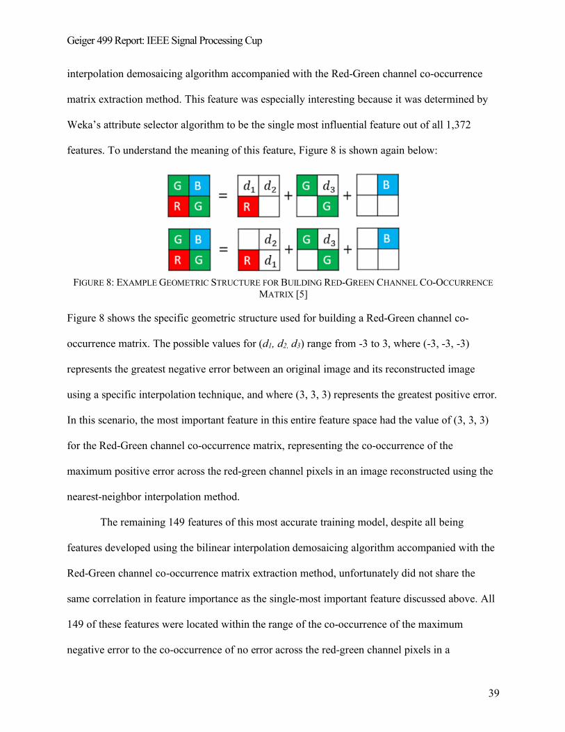
Geiger 499 Report: IEEE Signal Processing Cup
39
interpolation demosaicing algorithm accompanied with the Red-Green channel co-occurrence
matrix extraction method. This feature was especially interesting because it was determined by
Weka’s attribute selector algorithm to be the single most influential feature out of all 1,372
features. To understand the meaning of this feature, Figure 8 is shown again below:
FIGURE 8: EXAMPLE GEOMETRIC STRUCTURE FOR BUILDING RED-GREEN CHANNEL CO-OCCURRENCE
MATRIX [5]
Figure 8 shows the specific geometric structure used for building a Red-Green channel co-
occurrence matrix. The possible values for (d1, d2, d3) range from -3 to 3, where (-3, -3, -3)
represents the greatest negative error between an original image and its reconstructed image
using a specific interpolation technique, and where (3, 3, 3) represents the greatest positive error.
In this scenario, the most important feature in this entire feature space had the value of (3, 3, 3)
for the Red-Green channel co-occurrence matrix, representing the co-occurrence of the
maximum positive error across the red-green channel pixels in an image reconstructed using the
nearest-neighbor interpolation method.
The remaining 149 features of this most accurate training model, despite all being
features developed using the bilinear interpolation demosaicing algorithm accompanied with the
Red-Green channel co-occurrence matrix extraction method, unfortunately did not share the
same correlation in feature importance as the single-most important feature discussed above. All
149 of these features were located within the range of the co-occurrence of the maximum
negative error to the co-occurrence of no error across the red-green channel pixels in a
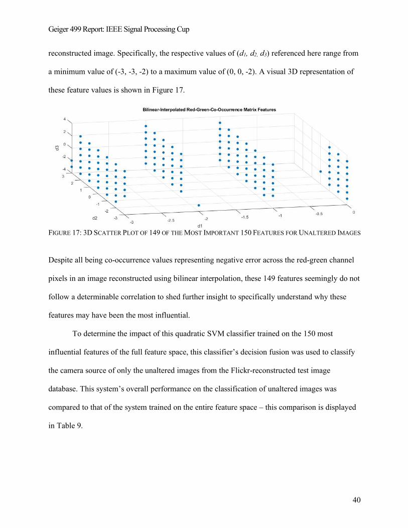
Geiger 499 Report: IEEE Signal Processing Cup
40
reconstructed image. Specifically, the respective values of (d1, d2, d3) referenced here range from
a minimum value of (-3, -3, -2) to a maximum value of (0, 0, -2). A visual 3D representation of
these feature values is shown in Figure 17.
FIGURE 17: 3D SCATTER PLOT OF 149 OF THE MOST IMPORTANT 150 FEATURES FOR UNALTERED IMAGES
Despite all being co-occurrence values representing negative error across the red-green channel
pixels in an image reconstructed using bilinear interpolation, these 149 features seemingly do not
follow a determinable correlation to shed further insight to specifically understand why these
features may have been the most influential.
To determine the impact of this quadratic SVM classifier trained on the 150 most
influential features of the full feature space, this classifier’s decision fusion was used to classify
the camera source of only the unaltered images from the Flickr-reconstructed test image
database. This system’s overall performance on the classification of unaltered images was
compared to that of the system trained on the entire feature space – this comparison is displayed
in Table 9.
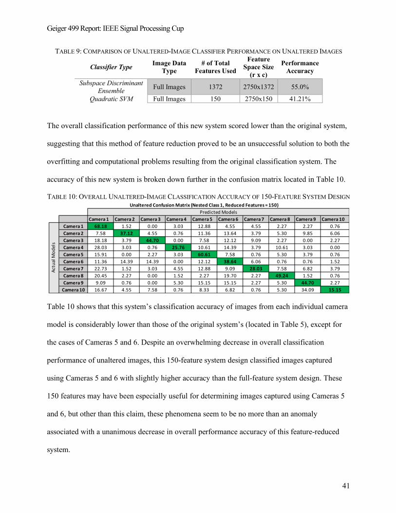
Geiger 499 Report: IEEE Signal Processing Cup
41
TABLE 9: COMPARISON OF UNALTERED-IMAGE CLASSIFIER PERFORMANCE ON UNALTERED IMAGES
Classifier Type Image Data Type
# of Total Features Used
Feature Space Size
(r x c)
Performance Accuracy
Subspace Discriminant Ensemble Full Images 1372 2750x1372 55.0%
Quadratic SVM Full Images 150 2750x150 41.21%
The overall classification performance of this new system scored lower than the original system,
suggesting that this method of feature reduction proved to be an unsuccessful solution to both the
overfitting and computational problems resulting from the original classification system. The
accuracy of this new system is broken down further in the confusion matrix located in Table 10.
TABLE 10: OVERALL UNALTERED-IMAGE CLASSIFICATION ACCURACY OF 150-FEATURE SYSTEM DESIGN
Table 10 shows that this system’s classification accuracy of images from each individual camera
model is considerably lower than those of the original system’s (located in Table 5), except for
the cases of Cameras 5 and 6. Despite an overwhelming decrease in overall classification
performance of unaltered images, this 150-feature system design classified images captured
using Cameras 5 and 6 with slightly higher accuracy than the full-feature system design. These
150 features may have been especially useful for determining images captured using Cameras 5
and 6, but other than this claim, these phenomena seem to be no more than an anomaly
associated with a unanimous decrease in overall performance accuracy of this feature-reduced
system.
Camera 1 Camera 2 Camera 3 Camera 4 Camera 5 Camera 6 Camera 7 Camera 8 Camera 9 Camera 10Camera 1 68.18 1.52 0.00 3.03 12.88 4.55 4.55 2.27 2.27 0.76Camera 2 7.58 37.12 4.55 0.76 11.36 13.64 3.79 5.30 9.85 6.06Camera 3 18.18 3.79 44.70 0.00 7.58 12.12 9.09 2.27 0.00 2.27Camera 4 28.03 3.03 0.76 25.76 10.61 14.39 3.79 10.61 3.03 0.00Camera 5 15.91 0.00 2.27 3.03 60.61 7.58 0.76 5.30 3.79 0.76Camera 6 11.36 14.39 14.39 0.00 12.12 38.64 6.06 0.76 0.76 1.52Camera 7 22.73 1.52 3.03 4.55 12.88 9.09 28.03 7.58 6.82 3.79Camera 8 20.45 2.27 0.00 1.52 2.27 19.70 2.27 49.24 1.52 0.76Camera 9 9.09 0.76 0.00 5.30 15.15 15.15 2.27 5.30 44.70 2.27
Camera 10 16.67 4.55 7.58 0.76 8.33 6.82 0.76 5.30 34.09 15.15
Unaltered Confusion Matrix (Nested Class 1, Reduced Features = 150)Predicted Models
Actu
al M
odel
s
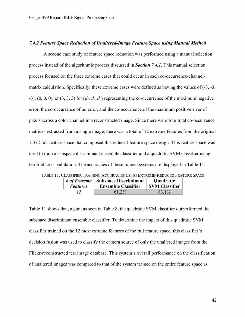
Geiger 499 Report: IEEE Signal Processing Cup
42
7.4.2 Feature Space Reduction of Unaltered-Image Feature Space using Manual Method
A second case study of feature space reduction was performed using a manual selection
process instead of the algorithmic process discussed in Section 7.4.1. This manual selection
process focused on the three extreme cases that could occur in each co-occurrence-channel-
matrix calculation. Specifically, these extreme cases were defined as having the values of (-3, -3,
-3), (0, 0, 0), or (3, 3, 3) for (d1, d2, d3) representing the co-occurrence of the maximum negative
error, the co-occurrence of no error, and the co-occurrence of the maximum positive error of
pixels across a color channel in a reconstructed image. Since there were four total co-occurrence
matrices extracted from a single image, there was a total of 12 extreme features from the original
1,372 full feature space that composed this reduced-feature-space design. This feature space was
used to train a subspace discriminant ensemble classifier and a quadratic SVM classifier using
ten-fold cross validation. The accuracies of these trained systems are displayed in Table 11.
TABLE 11: CLASSIFIER TRAINING ACCURACIES USING EXTREME-REDUCED FEATURE SPACE # of Extreme
Features Subspace Discriminant
Ensemble Classifier Quadratic
SVM Classifier 12 61.2% 83.1%
Table 11 shows that, again, as seen in Table 8, the quadratic SVM classifier outperformed the
subspace discriminant ensemble classifier. To determine the impact of this quadratic SVM
classifier trained on the 12 most extreme features of the full feature space, this classifier’s
decision fusion was used to classify the camera source of only the unaltered images from the
Flickr-reconstructed test image database. This system’s overall performance on the classification
of unaltered images was compared to that of the system trained on the entire feature space as
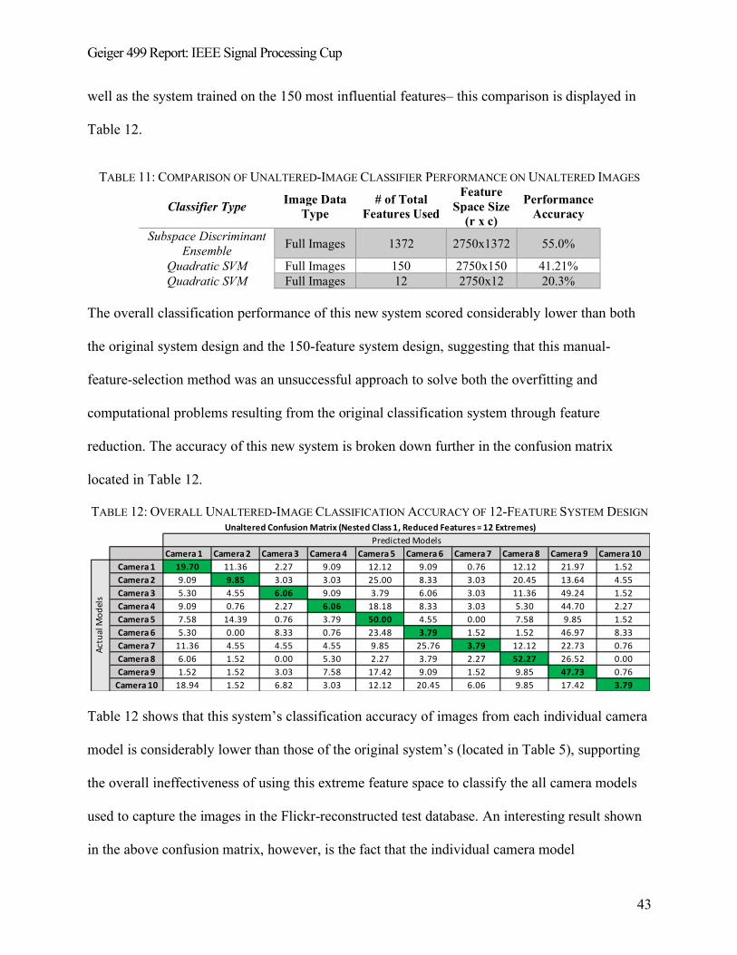
Geiger 499 Report: IEEE Signal Processing Cup
43
well as the system trained on the 150 most influential features– this comparison is displayed in
Table 12.
TABLE 11: COMPARISON OF UNALTERED-IMAGE CLASSIFIER PERFORMANCE ON UNALTERED IMAGES
Classifier Type Image Data Type
# of Total Features Used
Feature Space Size
(r x c)
Performance Accuracy
Subspace Discriminant Ensemble Full Images 1372 2750x1372 55.0%
Quadratic SVM Full Images 150 2750x150 41.21% Quadratic SVM Full Images 12 2750x12 20.3%
The overall classification performance of this new system scored considerably lower than both
the original system design and the 150-feature system design, suggesting that this manual-
feature-selection method was an unsuccessful approach to solve both the overfitting and
computational problems resulting from the original classification system through feature
reduction. The accuracy of this new system is broken down further in the confusion matrix
located in Table 12.
TABLE 12: OVERALL UNALTERED-IMAGE CLASSIFICATION ACCURACY OF 12-FEATURE SYSTEM DESIGN
Table 12 shows that this system’s classification accuracy of images from each individual camera
model is considerably lower than those of the original system’s (located in Table 5), supporting
the overall ineffectiveness of using this extreme feature space to classify the all camera models
used to capture the images in the Flickr-reconstructed test database. An interesting result shown
in the above confusion matrix, however, is the fact that the individual camera model
Camera 1 Camera 2 Camera 3 Camera 4 Camera 5 Camera 6 Camera 7 Camera 8 Camera 9 Camera 10Camera 1 19.70 11.36 2.27 9.09 12.12 9.09 0.76 12.12 21.97 1.52Camera 2 9.09 9.85 3.03 3.03 25.00 8.33 3.03 20.45 13.64 4.55Camera 3 5.30 4.55 6.06 9.09 3.79 6.06 3.03 11.36 49.24 1.52Camera 4 9.09 0.76 2.27 6.06 18.18 8.33 3.03 5.30 44.70 2.27Camera 5 7.58 14.39 0.76 3.79 50.00 4.55 0.00 7.58 9.85 1.52Camera 6 5.30 0.00 8.33 0.76 23.48 3.79 1.52 1.52 46.97 8.33Camera 7 11.36 4.55 4.55 4.55 9.85 25.76 3.79 12.12 22.73 0.76Camera 8 6.06 1.52 0.00 5.30 2.27 3.79 2.27 52.27 26.52 0.00Camera 9 1.52 1.52 3.03 7.58 17.42 9.09 1.52 9.85 47.73 0.76
Camera 10 18.94 1.52 6.82 3.03 12.12 20.45 6.06 9.85 17.42 3.79
Actu
al M
odel
s
Unaltered Confusion Matrix (Nested Class 1, Reduced Features = 12 Extremes)Predicted Models

Geiger 499 Report: IEEE Signal Processing Cup
44
classification accuracies for both Cameras 8 and 9 were higher in this case than those classified
using the 150-feature system design. This implies that these 12 extreme features could have held
more identification strength of these two camera models than the 150 most important features
determined using Weka. Or, these phenomena could be the result of an anomaly in the data, but
without more in-depth data mining, the true explanation to these remain unknown.
Geiger 499 Report: IEEE Signal Processing Cup
45
8. PRODUCTION SCHEDULE
8.1 The 2018 IEEE Signal Processing Cup Production Schedule
The 2018 IEEE Signal Processing Cup began in late August 2017 when the competition
topic was released. The only information provided at this time was the document referenced in
[2] and the training image database containing ten different camera models with 275 images per
camera. The deadline for submitting Open Competition results at this point was set to January
21, 2018. In order to meet this deadline, the goal for the Fall Term and ECE 498 was to decide
on a final system design for Union’s Signal Processing Cup Team’s camera model identification
system. The month of September was dedicated to completing all of the necessary research to be
able to design the image forensic techniques that would be used in the final system design. The
month of October was dedicated to writing Matlab code capable of using the chosen image
forensic techniques to build a desired feature space for a single camera directory. The rest of Fall
Term was dedicated to constructing our first full feature space with which to use to begin
training machine learning classifiers. The goal for Winter Break was to consolidate the original
feature-space-construction code to allow for and to begin the mass-production of different image
feature spaces. Around the second week of December, the competition organizers released the
Matlab script used to generate the manipulated image directories (Appendix A). Not too long
after this release, the competition organizers released the information that the Open Competition
deadline had been extended to February 8, 2018. This extension was favorable because the goal
set for Winter Break for beginning the mass-production of feature spaces had still remained
unfinished.
To start Winter Term ECE 499, feature spaces had been constructed using the twelve
different possible combinations of demosaicing algorithms and co-occurrence matrices of the full
Geiger 499 Report: IEEE Signal Processing Cup
46
image directory provided at the start of the competition. Given time constraints of the
competition deadline, the chosen feature space combination to use for the training of the machine
learning classifiers in the final system design were the four combinations used in [6]. The
immediate next step for Winter Term was to use the provided Matlab script for the manipulated
images to construct the respective nine image directories of 512x512 image blocks: one directory
containing image blocks of the original unaltered directory, and the remaining eight directories
containing manipulated image blocks of each manipulation technique constructed from this first
image block directory. Starting alongside the construction of these directories of image blocks
was determining, through trial-and-error, the best machine learning classifier available through
Matlab’s Classification Learner Application to use for the final classifier system designs. The
last week of January consisted of constructing manipulated image feature spaces, training and
selecting the best machine learning classifier designs for each feature space, and designing the
final three-fold, nested ensemble design covered in this report. Due to the time constraints of the
Open Competition deadline, only a small subset of the entire image block directory could be
used to construct the respective feature spaces to train each manipulated-image classifier. The
last week of Open Competition consisted of consolidating all of the deliverables due at the
competition deadline and submitting the two best classifier scores through Kaggle.
8.2 Suggestions for Improvement in Production Schedule
The main suggestion for improvement of the above production schedule would have been
to use the available time over winter break much more efficiently. If it were possible to
determine the best combination of demosaicing algorithms and co-occurrence matrices during
this time, then it could have greatly increased to overall accuracy of this same final system

Geiger 499 Report: IEEE Signal Processing Cup
47
design. A second suggestion for using the available Winter Break time more efficiently would
have been to have constructed the image block directories as soon as the code to do so was
released by the competition organizers. This could have allowed for the construction of image
block feature spaces using a much larger subspace of the entire image block directory to train the
manipulated-image classifiers than the time allowed for in the original production schedule.
These two improvements could have maximized the overall performance of this final system
design within the constraints of the 2018 IEEE Signal Processing Cup deadlines.

Geiger 499 Report: IEEE Signal Processing Cup
48
9. COST ANALYSIS
The cost of this entire senior capstone project amounted to $0 because this senior project
was entirely software-based. Matlab and its Classification Learner Application were the only
software tools used for the design and implementation of the camera model identification system
submitted for the 2018 Signal Processing Cup, and both of these were accessed through Union
College’s licensed use of the Matlab software.

Geiger 499 Report: IEEE Signal Processing Cup
49
10. USER MANUAL
The operation of this camera model identification is comprised of three main parts:
feature space construction, machine learning classifier training, and implementation of trained
machine learning classifiers to classify the test image database.
10.1 Feature Space Construction
The feature space construction for this final system design was implemented using the
Matlab scripts located in Appendix B. These scripts are written unique to the location of a
specific image file directory using a specific operating system (Windows or Linux), so it is
necessary to edit the file locations and to comment in/out the OS-based commands accordingly
for the desired application.
10.2 Machine Learning Classifier Training
Once these feature spaces have been constructed and imported into the Matlab
workspace, Matlab’s Classification Learner Application can then be used to train a desired
machine learning classifier. The specific classifier that will be trained in this example will be a
Subspace Discriminant Ensemble classifier trained using 30 learners and 686 subspace
dimensions determined from a full feature space of 1,372 total features. (Note: this user manual
was developed using Matlab R2017b.)
10.2.1 Opening Matlab’s Classification Learner Application
Figure 18 shows the location of the classification learner application within the main
Matlab window.
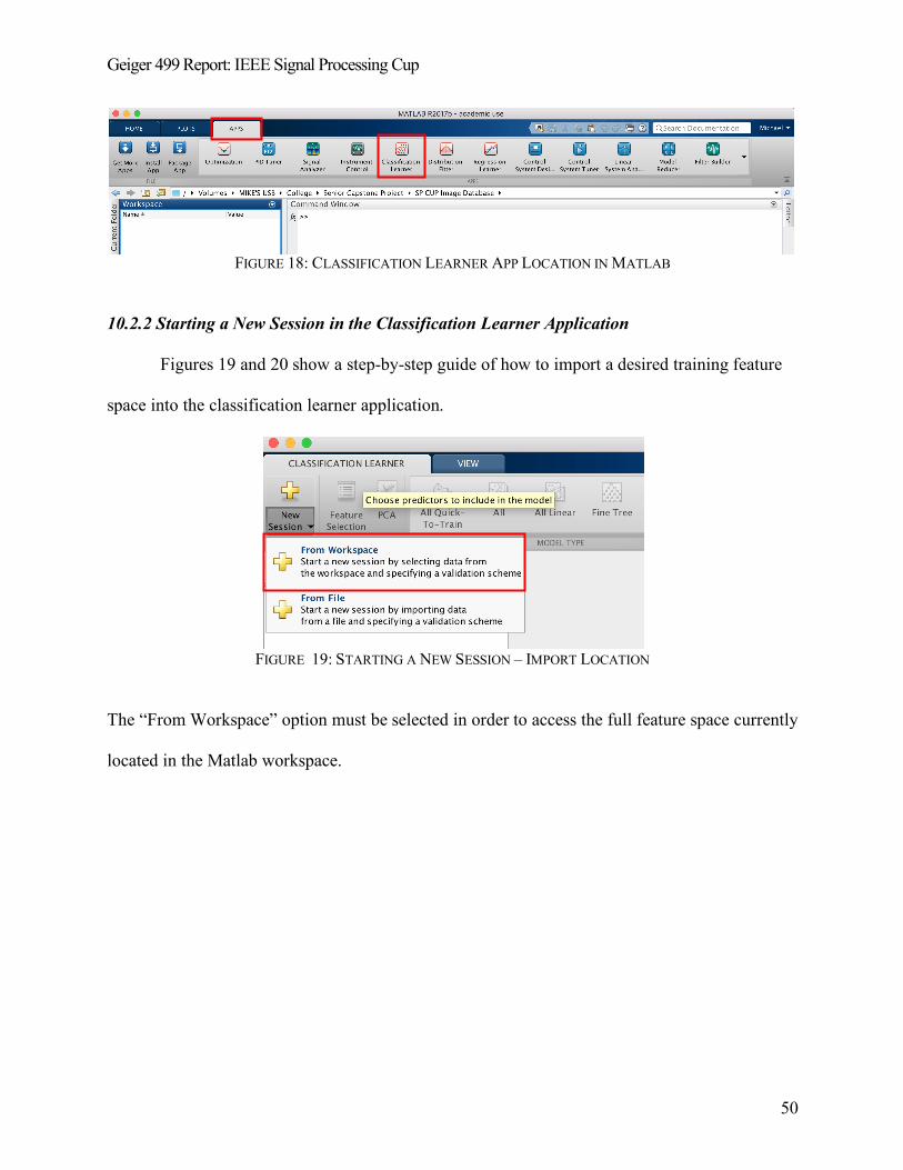
Geiger 499 Report: IEEE Signal Processing Cup
50
FIGURE 18: CLASSIFICATION LEARNER APP LOCATION IN MATLAB
10.2.2 Starting a New Session in the Classification Learner Application
Figures 19 and 20 show a step-by-step guide of how to import a desired training feature
space into the classification learner application.
FIGURE 19: STARTING A NEW SESSION – IMPORT LOCATION
The “From Workspace” option must be selected in order to access the full feature space currently
located in the Matlab workspace.
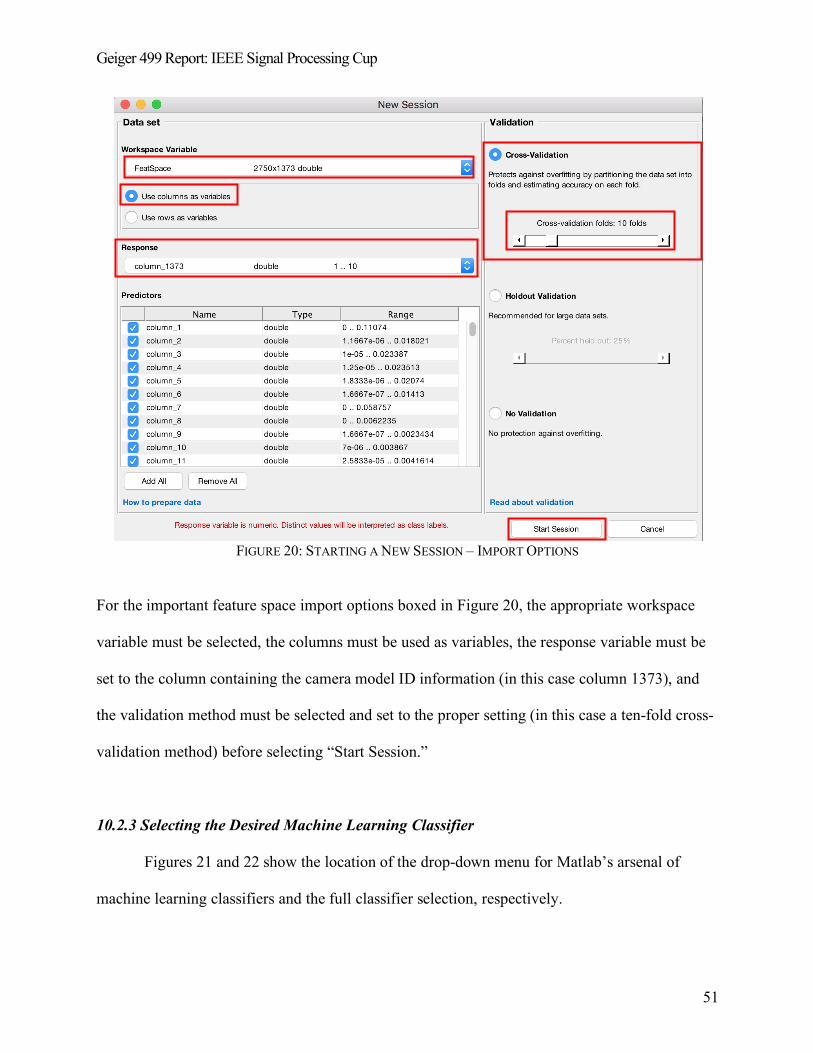
Geiger 499 Report: IEEE Signal Processing Cup
51
FIGURE 20: STARTING A NEW SESSION – IMPORT OPTIONS
For the important feature space import options boxed in Figure 20, the appropriate workspace
variable must be selected, the columns must be used as variables, the response variable must be
set to the column containing the camera model ID information (in this case column 1373), and
the validation method must be selected and set to the proper setting (in this case a ten-fold cross-
validation method) before selecting “Start Session.”
10.2.3 Selecting the Desired Machine Learning Classifier
Figures 21 and 22 show the location of the drop-down menu for Matlab’s arsenal of
machine learning classifiers and the full classifier selection, respectively.
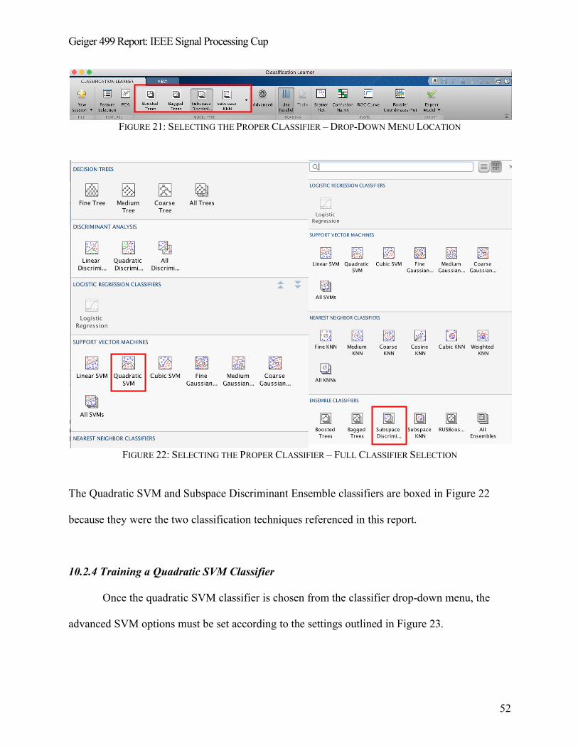
Geiger 499 Report: IEEE Signal Processing Cup
52
FIGURE 21: SELECTING THE PROPER CLASSIFIER – DROP-DOWN MENU LOCATION
FIGURE 22: SELECTING THE PROPER CLASSIFIER – FULL CLASSIFIER SELECTION
The Quadratic SVM and Subspace Discriminant Ensemble classifiers are boxed in Figure 22
because they were the two classification techniques referenced in this report.
10.2.4 Training a Quadratic SVM Classifier
Once the quadratic SVM classifier is chosen from the classifier drop-down menu, the
advanced SVM options must be set according to the settings outlined in Figure 23.
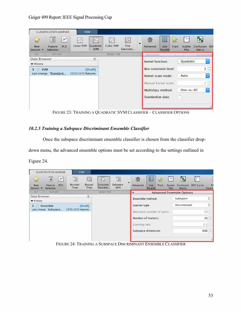
Geiger 499 Report: IEEE Signal Processing Cup
53
FIGURE 23: TRAINING A QUADRATIC SVM CLASSIFIER – CLASSIFIER OPTIONS
10.2.5 Training a Subspace Discriminant Ensemble Classifier
Once the subspace discriminant ensemble classifier is chosen from the classifier drop-
down menu, the advanced ensemble options must be set according to the settings outlined in
Figure 24.
FIGURE 24: TRAINING A SUBSPACE DISCRIMINANT ENSEMBLE CLASSIFIER
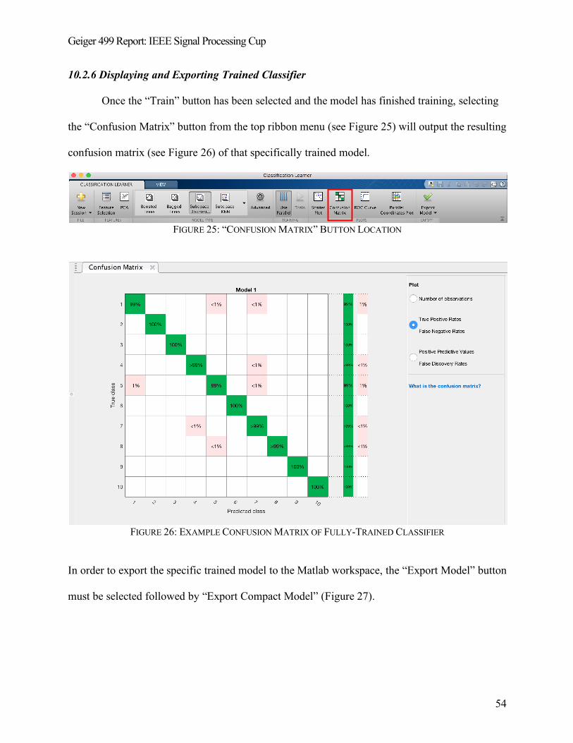
Geiger 499 Report: IEEE Signal Processing Cup
54
10.2.6 Displaying and Exporting Trained Classifier
Once the “Train” button has been selected and the model has finished training, selecting
the “Confusion Matrix” button from the top ribbon menu (see Figure 25) will output the resulting
confusion matrix (see Figure 26) of that specifically trained model.
FIGURE 25: “CONFUSION MATRIX” BUTTON LOCATION
FIGURE 26: EXAMPLE CONFUSION MATRIX OF FULLY-TRAINED CLASSIFIER
In order to export the specific trained model to the Matlab workspace, the “Export Model” button
must be selected followed by “Export Compact Model” (Figure 27).
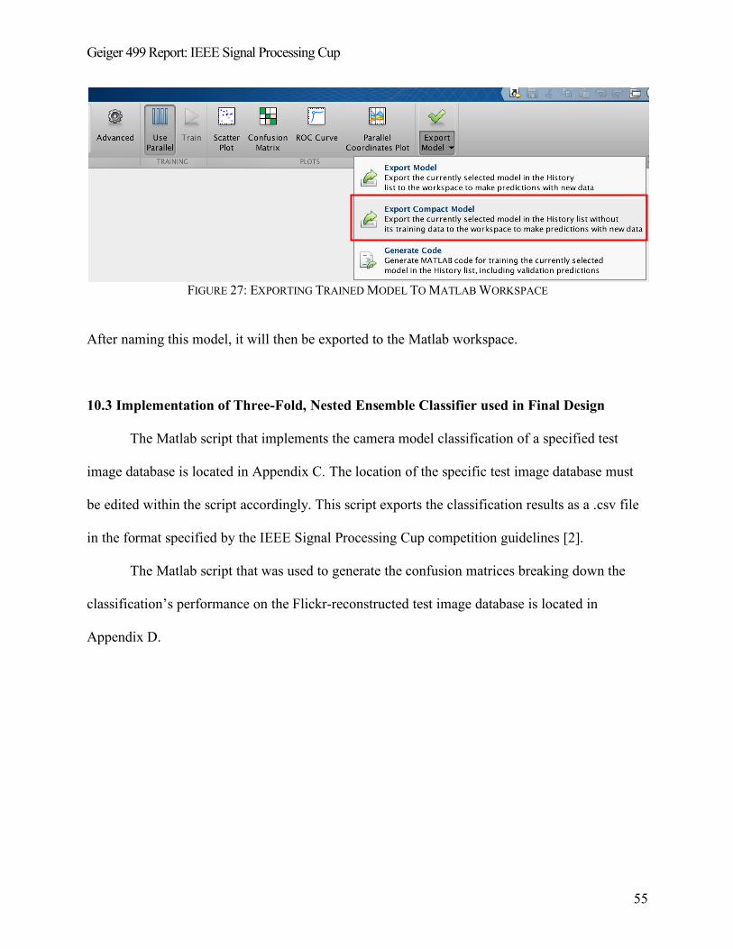
Geiger 499 Report: IEEE Signal Processing Cup
55
FIGURE 27: EXPORTING TRAINED MODEL TO MATLAB WORKSPACE
After naming this model, it will then be exported to the Matlab workspace.
10.3 Implementation of Three-Fold, Nested Ensemble Classifier used in Final Design
The Matlab script that implements the camera model classification of a specified test
image database is located in Appendix C. The location of the specific test image database must
be edited within the script accordingly. This script exports the classification results as a .csv file
in the format specified by the IEEE Signal Processing Cup competition guidelines [2].
The Matlab script that was used to generate the confusion matrices breaking down the
classification’s performance on the Flickr-reconstructed test image database is located in
Appendix D.
Geiger 499 Report: IEEE Signal Processing Cup
56
11. DISCUSSION, CONCLUSIONS, AND RECOMMENDATIONS
The challenge of the 2018 IEEE Signal Processing Cup required teams of undergraduate
students to use a combination of image forensics and machine learning to develop a classification
system capable of determining the make and model of a camera used to capture an image. The
designed system covered in this report was submitted on behalf of Union College’s first ever
Signal Processing Cup Team. The final system design consisted of using image forensic
techniques to convert images into information within a specific feature space and then using
these constructed feature spaces to train various machine learning classifiers. The specific image
forensics used in this final design first re-filtered images using a Bayer CFA and then re-
interpolated these images twice using two separate demosaicing algorithms: bilinear
interpolation and nearest-neighbor interpolation. An error image was then calculated from
subtracting the reconstructed images from the original images, from which information regarding
the co-occurrence of predetermined pixel value combinations were extracted in respect to the
image’s red channel and the image’s red-green channel. The co-occurrence matrices constructed
from an entire image directory were the full feature spaces used to train each of the ten-total
subspace discriminant ensemble classifiers whose resulting decision fusions made up a three-
fold, nested ensemble classifier. This nested classifier classified a test image database composed
of 2,640 images captured using different devices – but same make and model – than those used
to construct the training image database. Half of these images were unaltered, but the other half
of these images were manipulated using an undisclosed distribution of eight different
manipulation techniques. The top two classification scores of this final system design submitted
at the deadline of the competition were 65.6% and 65.0%.
Geiger 499 Report: IEEE Signal Processing Cup
57
11.1 Recommendations
The main recommendation for improvement of this specific design would be to use
various data mining methods to identify the most important features within the full feature spaces
used in the final design of this camera model identification system. Ideally, these feature spaces
would be greatly reduced from 1,372 features to less than 100 features. Since the 512x512 image
block directories contained more than 99,000 total images, reducing the number of features
would greatly increase the total amount of information that could be used to develop these
training feature spaces given the limitation of computational power experienced while using
Union’s lab computer resources. The increase of overall information used to train each classifier
theoretically should improve the performance accuracy of each of these classifiers, thus allowing
for the final nested-ensemble-classifier design to have a higher performance accuracy than
submitted for this year’s Signal Processing Cup Competition. This process of data mining would
also lend valuable insight unto the meaning behind the most significant features used to construct
this optimized feature space, providing valuable information of the unique features used to
distinguish the ten different camera models used in this competition.
This method of data mining would completely exhaust this proposed image classification
design, but there is no way of knowing that this optimized classifier would perform better than
most of the top finishers in this year’s competition. The top 100 finishers are shown on the
Signal Processing Cup leaderboard on Kaggle, and each of these finishers’ classification systems
scored higher than 95.9%. Kaggle’s discussion page for this competition contained the solutions
that many of these top-place finishers used for their final designs. Almost all of these teams were
using Python-based, dense neural network classifier arrays trained on an enormous amount of
image data that teams constructed using various online image databases in addition to the image
Geiger 499 Report: IEEE Signal Processing Cup
58
database provided by the competition organizers. In order to process hundreds-of-gigabytes-
worth of image data these teams must have had access to resources with incredibly powerful
computational power. For example, the second-place team for the IEEE Signal Processing Cup
competition, aptly named GPU Muscles, wrote their own discussion board post detailing the
specific neural network array used, the amount of extrapolated training data, as well as the their
incredibly powerful hardware whose graphics cards alone amounted to over $10,000. So, as a
final recommendation to improve the overall performance of this proposed image classification
system would be to scrap the design altogether, design a dense neural network array instead,
download an additional couple hundred gigabytes of image data, and purchase the necessary
resources capable of processing all of this information within a reasonable amount of time.
11.2 Lessons Learned
The biggest lesson I learned upon completion of this senior capstone project, aside from
learning about the entire topics of both image forensics and machine learning from the ground
up, was the importance of identifying and understanding the limitations of processing power that
are introduced when working with incredibly large datasets. Unfortunately, it did not seem like
the successful teams competing in this year’s Signal Processing Cup experienced same
computational limitations that I had throughout the development of this final classification
system design, which leads me to believe that our team was at a significant disadvantage since
the onset of this competition. Despite this clear disadvantage in processing power, however, I
was forced to use methods of data mining after the completion of the competition to understand
how to optimize the performance of this design. This forced me to not only search for specific
features that best distinguished between the ten different camera models for the specific machine

Geiger 499 Report: IEEE Signal Processing Cup
59
classifiers I was using but also to understand the physical meaning of each of these features by
linking them back to the specific image forensic techniques used to generate them. Although it
did not improve the overall performance, I felt that this data mining experience gave me the
deepest understanding of the overall operation and dependence of each machine learning
classifier. Because these top-finishing teams had access to incredible amount of processing
power, I think it would be reasonable to assume that these teams did not have the same learning
experience that I had through data mining. I feel that the focus of this year’s IEEE Signal
Processing Cup competition should have been more directly focused on the refinement of a
feature extraction process rather than focused on who could process the most amount of
information. But, at the end of the day, I owe everything I now know about image forensics and
machine learning due to this senior capstone project and the 2018 IEEE Signal Processing
Competition, which is makes this an incredibly rewarding learning experience as a whole.
Geiger 499 Report: IEEE Signal Processing Cup
60
12. REFERENCES
[1] M. C. Stamm, M. Wu and K. J. R. Liu, "Information Forensics: An Overview of the First
Decade," in IEEE Access, vol. 1, no. , pp. 167-200, 2013.
[2] Signal Processing Cup. (2017, October 23). Retrieved November 22, 2017, from
https://signalprocessingsociety.org/get-involved/signal-processing-cup
[3] M. Kirchner and T. Gloe, "Forensic camera model identification." Handbook of Digital
Forensics of Multimedia Data and Devices (2015): 329-374.
[4] A. Swaminathan, M. Wu and K. J. R. Liu, "Nonintrusive component forensics of visual
sensors using output images," in IEEE Transactions on Information Forensics and
Security, vol. 2, no. 1, pp. 91-106, March 2007.
[5] H. Cao and A. C. Kot, "Accurate Detection of Demosaicing Regularity for Digital Image
Forensics," in IEEE Transactions on Information Forensics and Security, vol. 4, no. 4, pp.
899-910, Dec. 2009.
[6] C. Chen and M. C. Stamm, "Camera model identification framework using an ensemble
of demosaicing features," 2015 IEEE International Workshop on Information Forensics
and Security (WIFS), Rome, 2015, pp. 1-6.
[7] T. Filler, J. Fridrich and M. Goljan, "Using sensor pattern noise for camera model
identification," 2008 15th IEEE International Conference on Image Processing, San
Diego, CA, 2008, pp. 1296-1299.
[8] T. H. Thai, R. Cogranne and F. Retraint, "Camera Model Identification Based on the
Heteroscedastic Noise Model," in IEEE Transactions on Image Processing, vol. 23, no. 1,
pp. 250-263, Jan. 2014.
[9] E. Kee, M. K. Johnson and H. Farid, "Digital Image Authentication From JPEG
Headers," in IEEE Transactions on Information Forensics and Security, vol. 6, no. 3, pp.
1066-1075, Sept. 2011.
[10] F. Marra, G. Poggi, C. Sansone, and L. Verdoliva "A study of co-occurrence
based local features for camera model identification." Multimedia Tools and Applications
(2016): 1-17.
Geiger 499 Report: IEEE Signal Processing Cup
61
[11] M. Kharrazi, H. T. Sencar and N. Memon, "Blind source camera identification,"
Image Processing, International Conference on Image Processing (ICIP), Singapore,
2004, pp. 709-712
[12] “Camera Raw 5.6 is here.” YLovePhoto,
www.ylovephoto.com/en/2009/11/19/camera-raw-5-6-is-here/
[13] Swirski, Leszek. “CFA Interpolation Detection.” Topics in Security: Forensic
Signal Analysis, University of Cambridge, 30 Nov. 2009. Accessed 10 Oct. 2017.
[14] “Ensemble Algorithms.” MathWorks, www.mathworks.com/help/stats/ensemble-
algorithms.html#btbbds9.
[15] IEEE's Signal Processing Society - Camera Model Identification, Kaggle,
www.kaggle.com/c/sp-society-camera-model-identification.
[16] “Weka 3: Data Mining Software in Java.” Weka 3 - Data Mining with Open
Source Machine Learning Software in Java, University of Waikato,
www.cs.waikato.ac.nz/ml/weka/.
[17] “Documentation - Choose Classifier Options.” MathWorks,
www.mathworks.com/help/stats/choose-a-classifier.html#bunt0n0-1.

Geiger 499 Report: IEEE Signal Processing Cup
62
13. APPENDICES
The following pages contain appendices with the following information:
- Appendix A: Matlab function script used to construct image block databases using one
of nine different manipulation techniques.
- Appendix B: Top-level Matlab script used to construct a full feature space of a specified
image directory along with Matlab scripts of all of the functions called through each
subsequent level.
- Appendix C: Matlab script containing all ten, trained, machine learning decision fusions
used in a three-fold, nested ensemble design.
- Appendix D: Matlab script used to generate confusion matrices that breakdown a
system’s classification results of the Flickr-reconstructed test image database.
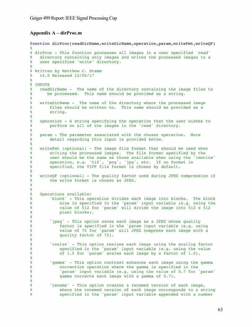
Geiger 499 Report: IEEE Signal Processing Cup
63
Appendix A – dirProc.m
function dirProc(readDirName,writeDirName,operation,param,writeFmt,writeQF) % % dirProc - This function processes all images in a user specified 'read' % directory containing only images and writes the processed images to a % user specified 'write' directory. % % Written by Matthew C. Stamm % v1.0 Released 12/05/17 % % INPUTS % readDirName - The name of the directory containing the image files to % be processed. This name should be provided as a string. % % writeDirName - The name of the directory where the processed image % files should be written to. This name should be provided as a % string. % % operation - A string specifying the operation that the user wishes to % perform on all of the images in the 'read' directory. % % param - The parameter associated with the chosen operation. More % detail regarding this input is provided below. % % writeFmt (optional) - The image file format that should be used when % writing the processed images. The file format specified by the % user should be the same as those available when using the 'imwrite' % operation, e.g. 'tif', 'png', 'jpg', etc. If no format is % specified, the TIFF file format is chosen by default. % % writeQF (optional) - The quality factor used during JPEG compression if % the write format is chosen as JPEG. % % % Operations available: % 'block' - This operation divides each image into blocks. The block % size is specified in the 'param' input variable (e.g. using the % value of 512 for 'param' will divide the image into 512 x 512 % pixel blocks). % % 'jpeg' - This option saves each image as a JPEG whose quality % factor is specified in the 'param input variable (e.g. using % value of 75 for 'param' will JPEG compress each image with a % quality factor of 75). % % 'resize' - This option resizes each image using the scaling factor % specified in the 'param' input variable (e.g. using the value % of 1.5 for 'param' scales each image by a factor of 1.5). % % 'gamma' - This option contrast enhances each image using the gamma % correction operation where the gamma is specified in the % 'param' input variable (e.g. using the value of 0.7 for 'param' % gamma corrects each image with a gamma of 0.7). % % 'rename' - This option creates a renamed version of each image, % where the renamed version of each image corresponds to a string % specified in the 'param' input variable appended with a number
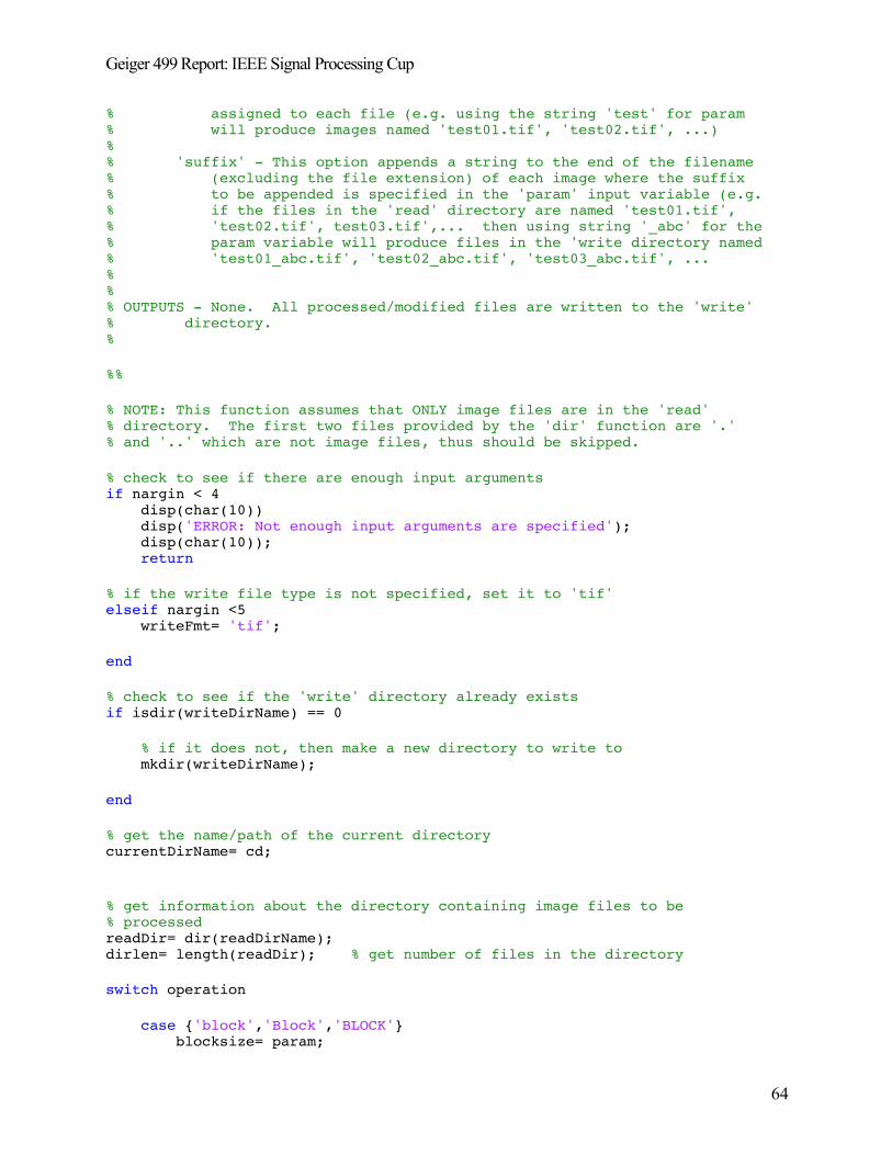
Geiger 499 Report: IEEE Signal Processing Cup
64
% assigned to each file (e.g. using the string 'test' for param % will produce images named 'test01.tif', 'test02.tif', ...) % % 'suffix' - This option appends a string to the end of the filename % (excluding the file extension) of each image where the suffix % to be appended is specified in the 'param' input variable (e.g. % if the files in the 'read' directory are named 'test01.tif', % 'test02.tif', test03.tif',... then using string '_abc' for the % param variable will produce files in the 'write directory named % 'test01_abc.tif', 'test02_abc.tif', 'test03_abc.tif', ... % % % OUTPUTS - None. All processed/modified files are written to the 'write' % directory. % %% % NOTE: This function assumes that ONLY image files are in the 'read' % directory. The first two files provided by the 'dir' function are '.' % and '..' which are not image files, thus should be skipped. % check to see if there are enough input arguments if nargin < 4 disp(char(10)) disp('ERROR: Not enough input arguments are specified'); disp(char(10)); return % if the write file type is not specified, set it to 'tif' elseif nargin <5 writeFmt= 'tif'; end % check to see if the 'write' directory already exists if isdir(writeDirName) == 0 % if it does not, then make a new directory to write to mkdir(writeDirName); end % get the name/path of the current directory currentDirName= cd; % get information about the directory containing image files to be % processed readDir= dir(readDirName); dirlen= length(readDir); % get number of files in the directory switch operation case {'block','Block','BLOCK'} blocksize= param;
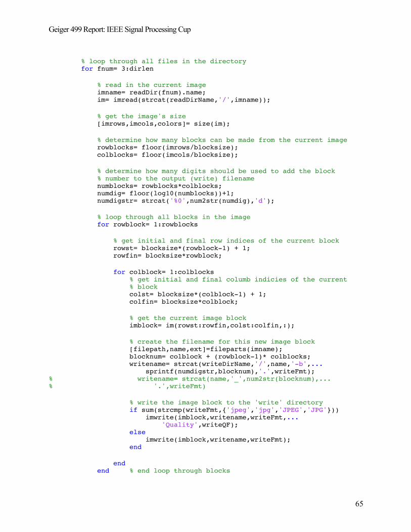
Geiger 499 Report: IEEE Signal Processing Cup
65
% loop through all files in the directory for fnum= 3:dirlen % read in the current image imname= readDir(fnum).name; im= imread(strcat(readDirName,'/',imname)); % get the image's size [imrows,imcols,colors]= size(im); % determine how many blocks can be made from the current image rowblocks= floor(imrows/blocksize); colblocks= floor(imcols/blocksize); % determine how many digits should be used to add the block % number to the output (write) filename numblocks= rowblocks*colblocks; numdig= floor(log10(numblocks))+1; numdigstr= strcat('%0',num2str(numdig),'d'); % loop through all blocks in the image for rowblock= 1:rowblocks % get initial and final row indices of the current block rowst= blocksize*(rowblock-1) + 1; rowfin= blocksize*rowblock; for colblock= 1:colblocks % get initial and final columb indicies of the current % block colst= blocksize*(colblock-1) + 1; colfin= blocksize*colblock; % get the current image block imblock= im(rowst:rowfin,colst:colfin,:); % create the filename for this new image block [filepath,name,ext]=fileparts(imname); blocknum= colblock + (rowblock-1)* colblocks; writename= strcat(writeDirName,'/',name,'-b',... sprintf(numdigstr,blocknum),'.',writeFmt); % writename= strcat(name,'_',num2str(blocknum),... % '.',writeFmt) % write the image block to the 'write' directory if sum(strcmp(writeFmt,{'jpeg','jpg','JPEG','JPG'})) imwrite(imblock,writename,writeFmt,... 'Quality',writeQF); else imwrite(imblock,writename,writeFmt); end end end % end loop through blocks
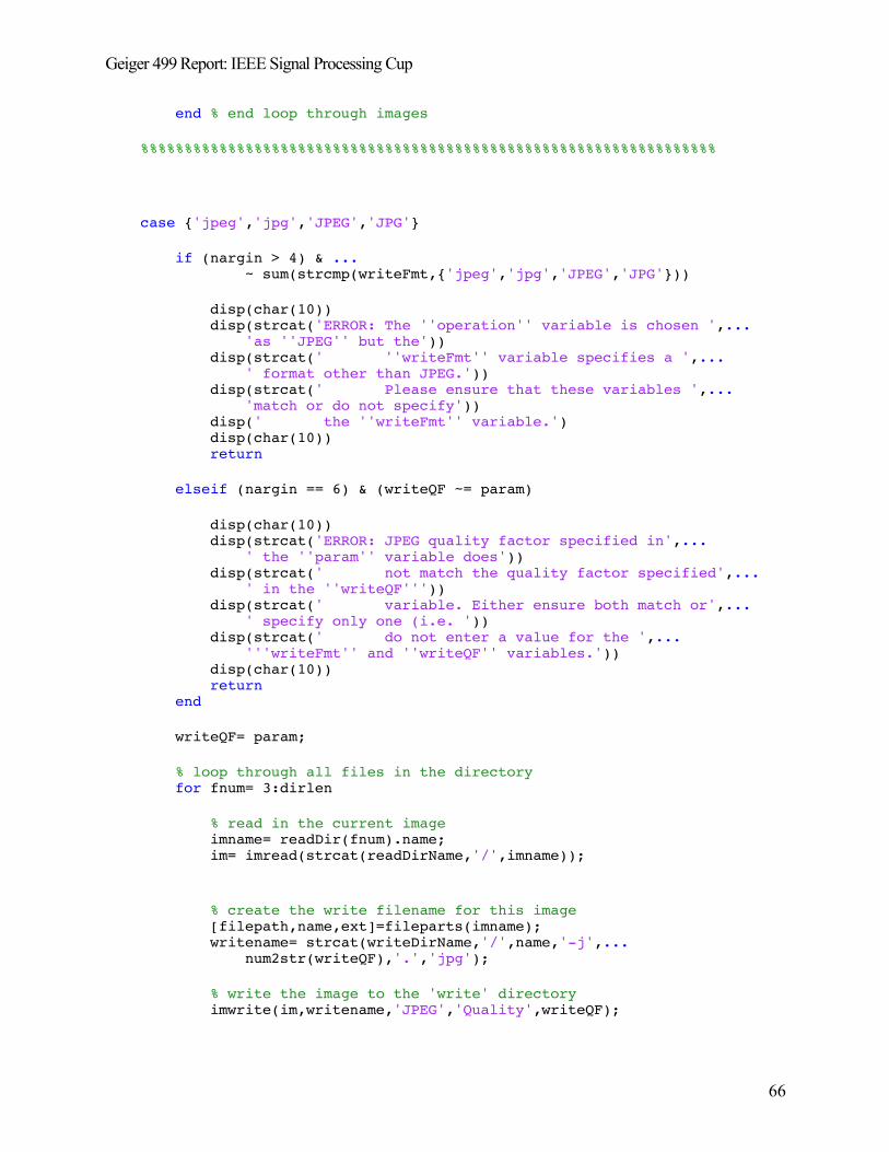
Geiger 499 Report: IEEE Signal Processing Cup
66
end % end loop through images %%%%%%%%%%%%%%%%%%%%%%%%%%%%%%%%%%%%%%%%%%%%%%%%%%%%%%%%%%%%%%%%%% case {'jpeg','jpg','JPEG','JPG'} if (nargin > 4) & ... ~ sum(strcmp(writeFmt,{'jpeg','jpg','JPEG','JPG'})) disp(char(10)) disp(strcat('ERROR: The ''operation'' variable is chosen ',... 'as ''JPEG'' but the')) disp(strcat(' ''writeFmt'' variable specifies a ',... ' format other than JPEG.')) disp(strcat(' Please ensure that these variables ',... 'match or do not specify')) disp(' the ''writeFmt'' variable.') disp(char(10)) return elseif (nargin == 6) & (writeQF ~= param) disp(char(10)) disp(strcat('ERROR: JPEG quality factor specified in',... ' the ''param'' variable does')) disp(strcat(' not match the quality factor specified',... ' in the ''writeQF''')) disp(strcat(' variable. Either ensure both match or',... ' specify only one (i.e. ')) disp(strcat(' do not enter a value for the ',... '''writeFmt'' and ''writeQF'' variables.')) disp(char(10)) return end writeQF= param; % loop through all files in the directory for fnum= 3:dirlen % read in the current image imname= readDir(fnum).name; im= imread(strcat(readDirName,'/',imname)); % create the write filename for this image [filepath,name,ext]=fileparts(imname); writename= strcat(writeDirName,'/',name,'-j',... num2str(writeQF),'.','jpg'); % write the image to the 'write' directory imwrite(im,writename,'JPEG','Quality',writeQF);
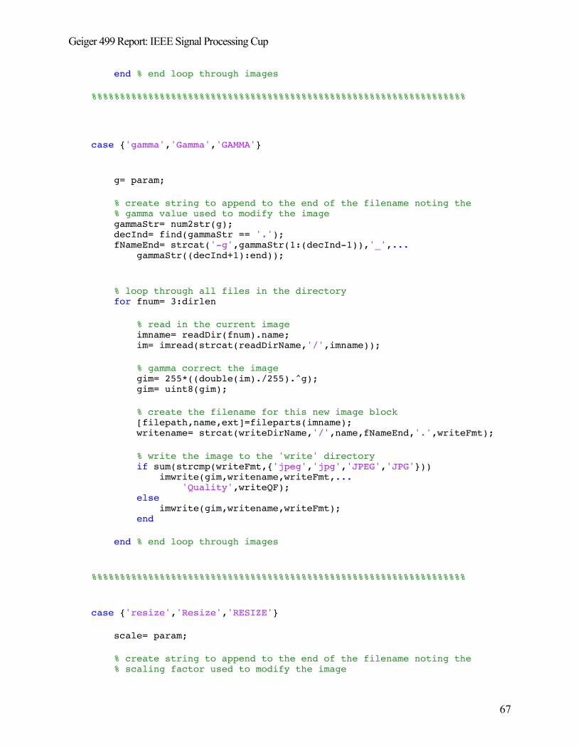
Geiger 499 Report: IEEE Signal Processing Cup
67
end % end loop through images %%%%%%%%%%%%%%%%%%%%%%%%%%%%%%%%%%%%%%%%%%%%%%%%%%%%%%%%%%%%%%%%%% case {'gamma','Gamma','GAMMA'} g= param; % create string to append to the end of the filename noting the % gamma value used to modify the image gammaStr= num2str(g); decInd= find(gammaStr == '.'); fNameEnd= strcat('-g',gammaStr(1:(decInd-1)),'_',... gammaStr((decInd+1):end)); % loop through all files in the directory for fnum= 3:dirlen % read in the current image imname= readDir(fnum).name; im= imread(strcat(readDirName,'/',imname)); % gamma correct the image gim= 255*((double(im)./255).^g); gim= uint8(gim); % create the filename for this new image block [filepath,name,ext]=fileparts(imname); writename= strcat(writeDirName,'/',name,fNameEnd,'.',writeFmt); % write the image to the 'write' directory if sum(strcmp(writeFmt,{'jpeg','jpg','JPEG','JPG'})) imwrite(gim,writename,writeFmt,... 'Quality',writeQF); else imwrite(gim,writename,writeFmt); end end % end loop through images %%%%%%%%%%%%%%%%%%%%%%%%%%%%%%%%%%%%%%%%%%%%%%%%%%%%%%%%%%%%%%%%%% case {'resize','Resize','RESIZE'} scale= param; % create string to append to the end of the filename noting the % scaling factor used to modify the image
Geiger 499 Report: IEEE Signal Processing Cup
68
scaleStr= num2str(scale); decInd= find(scaleStr == '.'); fNameEnd= strcat('-r',scaleStr(1:(decInd-1)),'_',... scaleStr((decInd+1):end)); % loop through all files in the directory for fnum= 3:dirlen % read in the current image imname= readDir(fnum).name; im= imread(strcat(readDirName,'/',imname)); % resize the image resizedIm = imresize(im,scale); % create the filename for the resized image [filepath,name,ext]=fileparts(imname); writename= strcat(writeDirName,'/',name,fNameEnd,'.',writeFmt); % write the image to the 'write' directory if sum(strcmp(writeFmt,{'jpeg','jpg','JPEG','JPG'})) imwrite(resizedIm,writename,writeFmt,... 'Quality',writeQF); else imwrite(resizedIm,writename,writeFmt); end end % end loop through images %%%%%%%%%%%%%%%%%%%%%%%%%%%%%%%%%%%%%%%%%%%%%%%%%%%%%%%%%%%%%%%%%% case {'rename','Rename','RENAME'} % get new filename (excluding image number) newname= param; % determine how many digits should be used to add the image % number to the output (write) filename numdig= floor(log10(dirlen-2))+1; numdigstr= strcat('%0',num2str(numdig),'d'); % loop through all files in the directory for fnum= 3:dirlen % read in the current image imname= readDir(fnum).name; im= imread(strcat(readDirName,'/',imname)); % create the filename for this new image block [filepath,name,ext]=fileparts(imname); imnum= fnum-2; writename= strcat(writeDirName,'/',newname,...
Geiger 499 Report: IEEE Signal Processing Cup
69
sprintf(numdigstr,imnum),'.',writeFmt); % write the image to the 'write' directory if sum(strcmp(writeFmt,{'jpeg','jpg','JPEG','JPG'})) imwrite(im,writename,writeFmt,... 'Quality',writeQF); else imwrite(im,writename,writeFmt); end end % end loop through images %%%%%%%%%%%%%%%%%%%%%%%%%%%%%%%%%%%%%%%%%%%%%%%%%%%%%%%%%%%%%%%%%% case {'suffix','Suffix','SUFFIX'} % get new filename (excluding image number) suffix= param; % loop through all files in the directory for fnum= 3:dirlen % read in the current image imname= readDir(fnum).name; im= imread(strcat(readDirName,'/',imname)); % create the filename for this new image block [filepath,name,ext]=fileparts(imname); imnum= fnum-2; writename= strcat(writeDirName,'/',name,suffix,'.',writeFmt); % write the image to the 'write' directory if sum(strcmp(writeFmt,{'jpeg','jpg','JPEG','JPG'})) imwrite(im,writename,writeFmt,... 'Quality',writeQF); else imwrite(im,writename,writeFmt); end end % end loop through images %%%%%%%%%%%%%%%%%%%%%%%%%%%%%%%%%%%%%%%%%%%%%%%%%%%%%%%%%%%%%%%%%% otherwise disp(char(10)) disp('ERROR: You have chosen an unknown operation'); disp(char(10)); return end
Geiger 499 Report: IEEE Signal Processing Cup
70
Appendix B
Feat_Space_Construct.m
clear;clc;close all; % Comment out the specific feature space construction command you are % building. All twelve feature spaces listed will need to be ran. The % written code should work with Prof. Dosiek's server import system for the % photos. % % % 1. Matlab demo & R coocc % try % diary('log.txt') % Feature_Space = FeatSpace('Matlab','R'); casenum = 1; % csvwrite(['SP_Cup_Block_Feature_Space_' num2str(casenum) '.csv'],Feature_Space); % diary off % catch err % err.getReport % disp('Uh-oh, we had an error!') % diary off % end % % % 2. Matlab demo & RG coocc % try % diary('log.txt') % Feature_Space = FeatSpace('Matlab','RG'); casenum = 2; % csvwrite(['SP_Cup_Block_Feature_Space_' num2str(casenum) '.csv'],Feature_Space); % diary off % catch err % err.getReport % disp('Uh-oh, we had an error!') % diary off % end % 3. Nearest Neighbor demo & R cooc try diary('log.txt') Feature_Space = FeatSpace('neighbor','R'); casenum = 'NN_R'; save(['SP_Cup_Test_Feature_Space_' casenum '.mat'],'Feature_Space'); diary off catch err err.getReport disp('Uh-oh, we had an error!') diary off end % 4. Nearest Neighbor demo & RG cooc try diary('log.txt') Feature_Space = FeatSpace('neighbor','RG'); casenum = 'NN_RG'; save(['SP_Cup_Test_Feature_Space_' casenum '.mat'],'Feature_Space'); diary off catch err err.getReport disp('Uh-oh, we had an error!')
Geiger 499 Report: IEEE Signal Processing Cup
71
diary off end % 5. Bilinear demo & R cooc try diary('log.txt') Feature_Space = FeatSpace('bilinear','R'); casenum = 'Bi_R'; save(['SP_Cup_Test_Feature_Space_' casenum '.mat'],'Feature_Space'); diary off catch err err.getReport disp('Uh-oh, we had an error!') diary off end % 6. Bilinear demo & RG cooc try diary('log.txt') Feature_Space = FeatSpace('bilinear','RG'); casenum = 'Bi_RG'; save(['SP_Cup_Test_Feature_Space_' casenum '.mat'],'Feature_Space'); diary off catch err err.getReport disp('Uh-oh, we had an error!') diary off end % % 7. Smooth Hue demo & R cooc % try % diary('log.txt') % Feature_Space = FeatSpace('smooth_hue','R'); casenum = 7; % csvwrite(['SP_Cup_Block_Feature_Space_' num2str(casenum) '.csv'],Feature_Space); % diary off % catch err % err.getReport % disp('Uh-oh, we had an error!') % diary off % end % % % 8. Smooth Hue demo & RG cooc % try % diary('log.txt') % Feature_Space = FeatSpace('smooth_hue','RG'); casenum = 8; % csvwrite(['SP_Cup_Block_Feature_Space_' num2str(casenum) '.csv'],Feature_Space); % diary off % catch err % err.getReport % disp('Uh-oh, we had an error!') % diary off % end % % % 9. Median Interpolation demo & R cooc % try % diary('log.txt') % Feature_Space = FeatSpace('median','R'); casenum = 9;
Geiger 499 Report: IEEE Signal Processing Cup
72
% csvwrite(['SP_Cup_Block_Feature_Space_' num2str(casenum) '.csv'],Feature_Space); % diary off % catch err % err.getReport % disp('Uh-oh, we had an error!') % diary off % end % % % 10. Median Interpolation demo & RG cooc % try % diary('log.txt') % Feature_Space = FeatSpace('median','RG'); casenum = 10; % csvwrite(['SP_Cup_Block_Feature_Space_' num2str(casenum) '.csv'],Feature_Space); % diary off % catch err % err.getReport % disp('Uh-oh, we had an error!') % diary off % toc % end % % % 11. Gradient-Based demo & R cooc % try % diary('log.txt') % Feature_Space = FeatSpace('gradient','R'); casenum = 11; % csvwrite(['SP_Cup_Block_Feature_Space_' num2str(casenum) '.csv'],Feature_Space); % diary off % catch err % err.getReport % disp('Uh-oh, we had an error!') % diary off % end % % % 12. Gradient-Based demo & RG cooc % try % diary('log.txt') % Feature_Space = FeatSpace('gradient','RG'); casenum = 12; % csvwrite(['SP_Cup_Block_Feature_Space_' num2str(casenum) '.csv'],Feature_Space); % diary off % catch err % err.getReport % disp('Uh-oh, we had an error!') % diary off % end
Geiger 499 Report: IEEE Signal Processing Cup
73
FeatSpace.m
function Feature_Space = FeatSpace(demotype,cooctype) % demotype = { % 'Matlab' - Matlab's demosaicing function % 'neighbor' - nearest neighbor interpolation % 'bilinear' - bilinear interpolation % 'smooth_hue' - smooth hue transition interpolation % 'median' - median-filtered bilinear interpolation % 'gradient' - gradient-based interpolation % } % cooctype = {'R','RG'} q = 2; T = 3; % Creature Feature Space Matrix % Feature_Space = zeros(2750,344); Feature_Space = zeros(2640,343); %if using Test Image Database % Make a cell array for camera model strings that we can iterate over CameraModel = cell(10); CameraModel{1} = 'HTC-1-M7\'; CameraModel{2} = 'iPhone-4s\'; CameraModel{3} = 'iPhone-6\'; CameraModel{4} = 'LG-Nexus-5x\'; CameraModel{5} = 'Motorola-Droid-Maxx\'; CameraModel{6} = 'Motorola-Nexus-6\'; CameraModel{7} = 'Motorola-X\'; CameraModel{8} = 'Samsung-Galaxy-Note3\'; CameraModel{9} = 'Samsung-Galaxy-S4\'; CameraModel{10} = 'Sony-NEX-7\'; % File Directory Import % PathToFiles = '\\unionpdc\SPcupPhotos\'; %if on Windows % PathToFiles = 'F:\Altered Image Database\Altered Image Database\Cameras_Blocks\'; %for Altered Image Blocks % [~, uid] = system('echo $UID'); uid = uid(1:end-1); %%%%%%%%%%%%%%%%%%%%%%%%%%%% % PathToFiles = ['/run/user/' uid '/gvfs/smb-share:server=EELAB-21080,share=Altered_Image_Database/']; %if on Linux PathToFiles = ['D:\SP_Cup_Test_Images\Images']; %if using Test Image Database % % Camera Feature Spaces % cam1_feature_space = camfeatspace(PathToFiles,CameraModel{1},1,q,T,demotype,cooctype); % cam2_feature_space = camfeatspace(PathToFiles,CameraModel{2},2,q,T,demotype,cooctype); % cam3_feature_space = camfeatspace(PathToFiles,CameraModel{3},3,q,T,demotype,cooctype); % cam4_feature_space = camfeatspace(PathToFiles,CameraModel{4},4,q,T,demotype,cooctype); % cam5_feature_space = camfeatspace(PathToFiles,CameraModel{5},5,q,T,demotype,cooctype); % cam6_feature_space = camfeatspace(PathToFiles,CameraModel{6},6,q,T,demotype,cooctype);
Geiger 499 Report: IEEE Signal Processing Cup
74
% cam7_feature_space = camfeatspace(PathToFiles,CameraModel{7},7,q,T,demotype,cooctype); % cam8_feature_space = camfeatspace(PathToFiles,CameraModel{8},8,q,T,demotype,cooctype); % cam9_feature_space = camfeatspace(PathToFiles,CameraModel{9},9,q,T,demotype,cooctype); % cam10_feature_space = camfeatspace(PathToFiles,CameraModel{10},10,q,T,demotype,cooctype); % % % Compile Feature Spaces together % Feature_Space(1:275,:) = cam1_feature_space; % Feature_Space(276:550,:) = cam2_feature_space; % Feature_Space(551:825,:) = cam3_feature_space; % Feature_Space(826:1100,:) = cam4_feature_space; % Feature_Space(1101:1375,:) = cam5_feature_space; % Feature_Space(1376:1650,:) = cam6_feature_space; % Feature_Space(1651:1925,:) = cam7_feature_space; % Feature_Space(1926:2200,:) = cam8_feature_space; % Feature_Space(2201:2475,:) = cam9_feature_space; % Feature_Space(2476:2750,:) = cam10_feature_space; % Test Image Database Feature Space Feature_Space = camfeatspace(PathToFiles,'VOID','VOID',q,T,demotype,cooctype); %if using Test Image Database end
Geiger 499 Report: IEEE Signal Processing Cup
75
camfeatspace.m
function cam_feat_space = camfeatspace(PathToFiles,camname,camnum,q,T,demotype,cooctype) % PathToPics = [PathToFiles camname]; %this gives us the full path to the folder containing the images for a particular camera. Then we can query for file names and iterate over them for analysis % imgFile = dir(PathToPics); PathToPics = PathToFiles; %if using Test Image Database imgFile = dir(PathToFiles); %if using Test Image Database camname = 'TEST_DATA'; %if using Test Image Database % %%%%%%%%%%%%%%%%%%%%%%%%%% % remove '.*' files idxToKill = []; for k = 1:length(imgFile) M = length(imgFile(k).name); if strcmp(imgFile(k).name(1),'.') idxToKill = [idxToKill k]; end end imgFile(idxToKill) = []; % only keep '*.tif' idxToKill = []; for k = 1:length(imgFile) M = length(imgFile(k).name); if M < 5 %kill if file name is too small to have been '*.tif' idxToKill = [idxToKill k]; elseif ~strcmp(imgFile(k).name(M-3:M),{'.tif', '.TIF'}) %kill if file isnt tif idxToKill = [idxToKill k]; end end imgFile(idxToKill) = []; %%%%%%%%%%%%%%%%%%%%%%%%%%%% % cam_feat_space = zeros(275,344); cam_feat_space = zeros(2640,343); %if using Test Image Database for l = 1:length(imgFile) %CurrentIMG = fullfile(camnum,imgFile(l).name); %%%%%%%%%%%%%%%%%%%%%%%%%%%% CurrentIMG = fullfile(PathToPics,imgFile(l).name); A = imread(CurrentIMG); % Linux: % disp([camname ', ' demotype ', ' cooctype ': Analyzing image ' num2str(l) ' of ' num2str(length(imgFile)) ', ' num2str(get_free_mem()) ' MB of free memory']) % Windows: [userview,systemview] = memory; disp([camname ', ' demotype ', ' cooctype ': Analyzing image ' num2str(l) ' of ' num2str(length(imgFile)) ', ' num2str(systemview.PhysicalMemory.Available/1024/1024) ' MB of free memory']) E = demotrunc(A, demotype, q, T); cooc = makecooc(E, cooctype);
Geiger 499 Report: IEEE Signal Processing Cup
76
%cam_feat_space(l,344) = 1; %%%%%%%%%%%%%%%%%%%%%%%%%%%% % cam_feat_space(l,344) = camnum; cam_feat_space(l,1:343) = cooc'; end end
Geiger 499 Report: IEEE Signal Processing Cup
77
demotrunc.m
function E = demotrunc(A, type, q, T) % Types: % 'Matlab' - Matlab's demosaicing function % 'neighbor' - nearest neighbor interpolation % 'bilinear' - bilinear interpolation % 'smooth_hue' - smooth hue transition interpolation % 'median' - median-filtered bilinear interpolation % 'gradient' - gradient-based interpolation % q = 2, T = 3 % gbrg Bayer CFA filter A_raw = uint8(zeros(size(A))); [nrows, ncols] = size(A(:,:,1)); for i=1:nrows for j = 1:ncols if mod(i,2)~=0 && mod(j,2)~=0 %i odd, j odd, keep G A_raw(i,j,2) = A(i,j,2); elseif mod(i,2)~=0 && mod(j,2) ==0 % i odd, j even, keep B A_raw(i,j,3) = A(i,j,3); elseif mod(i,2)==0 && mod(j,2)~=0 % i even, j odd, keep R A_raw(i,j,1) = A(i,j,1); elseif mod(i,2)==0 && mod(j,2)==0 % i even, j even, keep G A_raw(i,j,2) = A(i,j,2); end end end Afloat = double(A); % For error image calculation % Image resampling based on specified demosaicing algorithm switch type case 'Matlab' I = uint8(sum(A_raw,3)); A_demosaic = demosaic(I,'gbrg'); % error image calculation E = Afloat - double(A_demosaic); case 'neighbor' I = sum(A_raw,3); A_demosaic = demosaicing_v2(I,type); % error image calculation E = Afloat - A_demosaic; case 'bilinear' I = sum(A_raw,3); A_demosaic = demosaicing_v2(I,type); % error image calculation E = Afloat - A_demosaic; case 'smooth_hue' I = sum(A_raw,3); A_demosaic = demosaicing_v2(I,type); % error image calculation
Geiger 499 Report: IEEE Signal Processing Cup
78
E = Afloat - A_demosaic; case 'median' I = sum(A_raw,3); A_demosaic = demosaicing_v2(I,type); % error image calculation E = Afloat - A_demosaic; case 'gradient' I = sum(A_raw,3); A_demosaic = demosaicing_v2(I,type); % error image calculation E = Afloat - A_demosaic; end % Image value compression via truncation and quantization Emax = T; Emin = -T; E = round(E/q); E(E > Emax) = Emax; E(E < Emin) = Emin; end
Geiger 499 Report: IEEE Signal Processing Cup
79
makecooc.m
function cooc = makecooc(E, type) % E = output of demotrunc() % type = "'R', 'RG'} [nrows, ncols] = size(E(:,:,1)); % bust out R and G layers R = E(:,:,1); G = E(:,:,2); %reshape layers so 3d, with each slice a CFA tile R3d = permute(reshape(permute(reshape(R, size(R, 1), 2, []), [2 1 3]), 2, 2, []), [2 1 3]); G3d = permute(reshape(permute(reshape(G, size(G, 1), 2, []), [2 1 3]), 2, 2, []), [2 1 3]); %get number of tiles Ntiles = size(R3d,3); %get number of permuations Nd = 7^3; %initialize label vector d_labels = zeros(Nd,3); %get cardinality of G1 and G2 sets G1rows = 1:2:nrows; G1cols = 1:2:ncols; G2rows = 2:2:nrows; G2cols = 2:2:ncols; NG1 = length(G1rows) * length(G1cols); NG2 = length(G2rows) * length(G2cols); switch type case 'R' %initialize co-occurance matrices CR = zeros(Nd,1); %loop through different combos of d1, d2, and d3 idx = 1; for d1 = -3:3 for d2 = -3:3 for d3 = -3:3 % initial stuff %%%%%%%%%%%%%%%%%%%%%%%%%%%%%%%%%%%%%%%%%%%%%%% d_labels(idx,:) = [d1, d2, d3]; %make reference matrices for our desired values dmatR3d = repmat([d1, d2; 0, d3],1,1,Ntiles); % CR %%%%%%%%%%%%%%%%%%%%%%%%%%%%%%%%%%%%%%%%%%%%%%%%%%%%%%%%%% %make vector of tile matches matchvec = sum(sum(R3d==dmatR3d)); %count up matches (if matchvec == 4, we have a match!) %and assign to co-occurance matrix
Geiger 499 Report: IEEE Signal Processing Cup
80
CR(idx) = sum(matchvec(:) == 4)/NG1; idx = idx+1; end end end cooc = CR; case 'RG' %initialize co-occurance matrices CRG = zeros(Nd,1); %loop through different combos of d1, d2, and d3 idx = 1; for d1 = -3:3 for d2 = -3:3 for d3 = -3:3 % initial stuff %%%%%%%%%%%%%%%%%%%%%%%%%%%%%%%%%%%%%%%%%%%%%%% d_labels(idx,:) = [d1, d2, d3]; %make reference matrices for our desired values dmatR1 = repmat([d1, d2],1,1,Ntiles); dmatR2 = repmat([d2; d1],1,1,Ntiles); % CRG %%%%%%%%%%%%%%%%%%%%%%%%%%%%%%%%%%%%%%%%%%%%%%%%%%%%%%%%% % match up G vals matchvecG = squeeze(G3d(1,2,:)) == d3; % match up R values for 1st term matchvecR1 = sum(R3d(1,:,:) == dmatR1); % match up R values for 2nd term matchvecR2 = sum(R3d(:,2,:) == dmatR2); % combine (matchvec == 3 means we have a match! matchvecRG1 = matchvecG + matchvecR1(:); matchvecRG2 = matchvecG + matchvecR2(:); CRG(idx) = sum(matchvecRG1 == 3)/NG1 + sum(matchvecRG2 == 3)/NG2; idx = idx+1; end end end cooc = CRG; end end
Geiger 499 Report: IEEE Signal Processing Cup
81
demosaicing_v2.m
function output = demosaicing_v2(input,type) % Code modified from CFA Interpolation Detection by Leszek Swirski (Nov 30, % 2009), accessed on 07/05/2017 % The paper can be found here: % https://www.cl.cam.ac.uk/teaching/0910/R08/work/essay-ls426-cfadetection.pdf % Types: % 'neighbor' - nearest neighbor interpolation % 'bilinear' - bilinear interpolation % 'smooth_hue' - smooth hue transition interpolation % 'median' - median-filtered bilinear interpolation % 'gradient' - gradient-based interpolation % Input MUST be in double for code to run successfully % Load image S = input; % Create CFA filter for each of the three colours in GBRG format Rcfa = repmat([0 0;1 0],size(S)/2); Gcfa = repmat([1 0;0 1],size(S)/2); Bcfa = repmat([0 1;0 0],size(S)/2); % Split data into 'hat' variables Rh = S.*Rcfa; Gh = S.*Gcfa; Bh = S.*Bcfa; switch type case 'neighbor' % nearest neighbor interpolation R = Rh(floor([0:end-1]/2)*2+2,floor([0:end-1]/2)*2+1); G = zeros(size(Gh)); G(floor([0:end-1]/2)*2+1,:) = Gh(floor([0:end-1]/2)*2+1,floor([0:end-1]/2)*2+1); G(floor([0:end-1]/2)*2+2,:) = Gh(floor([0:end-1]/2)*2+2,floor([0:end-1]/2)*2+2); B = Bh(floor([0:end-1]/2)*2+1,floor([0:end-1]/2)*2+2); case 'bilinear' % bilinear interpolation R = conv2(Rh,[1 2 1;2 4 2;1 2 1]/4,'same'); G = conv2(Gh,[0 1 0;1 4 1;0 1 0]/4,'same'); B = conv2(Bh,[1 2 1;2 4 2;1 2 1]/4,'same'); case 'smooth_hue' % smooth hue transition interpolation G = conv2(Gh,[0 1 0;1 4 1;0 1 0]/4,'same') ; tmp = Rh./G; tmp(isnan(tmp)) = 0; tmp(isinf(tmp)) = 255; R = G.*conv2(tmp,[1 2 1;2 4 2;1 2 1]/4,'same') ; tmp = Bh./G; tmp(isnan(tmp)) = 0; tmp(isinf(tmp)) = 255; B = G.*conv2(tmp,[1 2 1;2 4 2;1 2 1]/4,'same') ; case 'median' % median-filtered bilinear interpolation R = conv2(Rh,[1 2 1;2 4 2;1 2 1]/4,'same') ; G = conv2(Gh,[0 1 0;1 4 1;0 1 0]/4,'same') ; B = conv2(Bh,[1 2 1;2 4 2;1 2 1]/4,'same') ; Mrg = R-G; Mrb = R-B; Mgb = G-B;
Geiger 499 Report: IEEE Signal Processing Cup
82
R = S+Mrg.*Gcfa+Mrb.*Bcfa ; G = S-Mrg.*Rcfa+Mgb.*Bcfa ; B = S-Mrb.*Rcfa-Mgb.*Gcfa ; case 'gradient' % gradient-based interpolation H = abs((S(:,[1 1 1:end-2])+S(:,[3:end end end]))/2-S); V = abs((S([1 1 1:end-2],:)+S([3:end end end],:))/2-S); G = Gh+(Rcfa+Bcfa).*((H<V).*((Gh(:,[1 1:end-1])+Gh(:,[2:end end]))/2)+(H>V).*((Gh([1 1:end-1],:)+Gh([2:end end],:))/2)+(H==V).*((Gh(:,[1 1:end-1])+Gh(:,[2:end end])+Gh([1 1:end-1],:)+Gh([2:end end],:))/4)); R = G+conv2(Rh-Rcfa.*G,[1 2 1;2 4 2;1 2 1]/4,'same'); B = G+conv2(Bh-Bcfa.*G,[1 2 1;2 4 2;1 2 1]/4,'same'); end %% Output output(:,:,1)=R; output(:,:,2)=G; output(:,:,3)=B; end
Geiger 499 Report: IEEE Signal Processing Cup
83
Appendix C – NestedClassifier.m
% Image Classification Script clear;clc;close all % Load Test Image Directory and Classifiers load Test_imgFile.mat % load trainedSD_35L_300sd.mat % load trainedFullSVM_Reduced150.mat load trainedFullSVM_Reduced12Extreme.mat % load trainedAltSD.mat % load trainedAlt_Type_675.mat % load trainedAlt_Type_1_1.mat % load trainedAlt_Type_2_1.mat % load trainedAlt_Type_3_1.mat % load trainedAlt_Type_4_1.mat % load trainedAlt_Type_5_1.mat % load trainedAlt_Type_6_1.mat % load trainedAlt_Type_7_1.mat % load trainedAlt_Type_8_1.mat %% Build Camera ID References CameraModel = cell(10,1); CameraModel{1} = 'HTC-1-M7'; CameraModel{2} = 'iPhone-4s'; CameraModel{3} = 'iPhone-6'; CameraModel{4} = 'LG-Nexus-5x'; CameraModel{5} = 'Motorola-Droid-Maxx'; CameraModel{6} = 'Motorola-Nexus-6'; CameraModel{7} = 'Motorola-X'; CameraModel{8} = 'Samsung-Galaxy-Note3'; CameraModel{9} = 'Samsung-Galaxy-S4'; CameraModel{10} = 'Sony-NEX-7'; % Build Test Feature Space Bi_R = load('SP_Cup_Test_Feature_Space_Bi_R.mat'); Bi_RG = load('SP_Cup_Test_Feature_Space_Bi_RG.mat'); NN_R = load('SP_Cup_Test_Feature_Space_NN_R.mat'); NN_RG = load('SP_Cup_Test_Feature_Space_NN_RG.mat'); % Bi_R = load('Test Image Feature Spaces\SP_Cup_Test_Feature_Space_Bi_R.mat'); % Bi_RG = load('Test Image Feature Spaces\SP_Cup_Test_Feature_Space_Bi_RG.mat'); % NN_R = load('Test Image Feature Spaces\SP_Cup_Test_Feature_Space_NN_R.mat'); % NN_RG = load('Test Image Feature Spaces\SP_Cup_Test_Feature_Space_NN_RG.mat'); TestFeatureSpace(:,1:343) = Bi_R.Feature_Space; TestFeatureSpace(:,344:686) = Bi_RG.Feature_Space; TestFeatureSpace(:,687:1029) = NN_R.Feature_Space; TestFeatureSpace(:,1030:1372) = NN_RG.Feature_Space; [~,x] = size(TestFeatureSpace);
Geiger 499 Report: IEEE Signal Processing Cup
84
%% Classifier Test #1: %Classifying Unaltered Images using Best Unaltered Classifier & %Manually Classifying Altered Images to Cam1 % Build Classified Matrix yfit = zeros(2641,2); yfit = num2cell(yfit); %converts yfit to cell array yfit(1,:) = {'fname' 'camera'}; for k = 2:2641 disp([num2str(k-1) ' of 2640']) yfit{k,1} = Test_imgFile(k-1).name; if sum(ismember('unalt',yfit{k,1})) == 5 %separating unaltered images yfit{k,2} = trainedFullSVM_Reduced12Extreme.predictFcn(array2table(TestFeatureSpace(k-1,1:x))); else %classifying altered images yfit{k,2} = 1; end end %% Classifier Test #2: %Classifying Unaltered Images using Best Unaltered Classifier & %Classifying Altered Images using Altered-only-trained Classifier % Build Classified Matrix yfit = zeros(2641,2); yfit = num2cell(yfit); %converts yfit to cell array yfit(1,:) = {'fname' 'camera'}; for k = 2:2641 disp([num2str(k-1) ' of 2640']) yfit{k,1} = imgFile(k-1).name; if ismember('unalt',yfit{k,1}) %separating unaltered images yfit{k,2} = trainedSD_35L_300sd.predictFcn(array2table(TestFeatureSpace(k-1,1:x))); else %classifying altered images yfit{k,2} = trainedAltSD.predictFcn(TestFeatureSpace(k-1,1:end)); end end %% Classifier Test #3: %Classifying Unaltered Images using Best Unaltered Classifier & %Classifying Altered Images Based on Alteration Type and then %Classifying Camera Model w/in each Type % Build Classified Matrix yfit = zeros(2641,2); yfit = num2cell(yfit); %converts yfit to cell array yfit(1,:) = {'fname' 'camera'};
Geiger 499 Report: IEEE Signal Processing Cup
85
for k = 2:2641 disp([num2str(k-1) ' of 2640']) yfit{k,1} = Test_imgFile(k-1).name; if ismember('unalt',yfit{k,1}) %separating unaltered images % yfit{k,2} = trainedSD_35L_300sd.predictFcn(array2table(TestFeatureSpace(k-1,1:x))); elseif ismember('manip',yfit{k,1})%classifying altered images yfit{k,2} = trainedAlt_Type_675.predictFcn(TestFeatureSpace(k-1,1:x)); % if yfit{k,2} == 1 % yfit{k,2} = trainedAlt_Type_1_1.predictFcn(TestFeatureSpace(k-1,1:x)); % elseif yfit{k,2} == 2 % yfit{k,2} = trainedAlt_Type_2_1.predictFcn(TestFeatureSpace(k-1,1:x)); % elseif yfit{k,2} == 3 % yfit{k,2} = trainedAlt_Type_3_1.predictFcn(TestFeatureSpace(k-1,1:x)); % elseif yfit{k,2} == 4 % yfit{k,2} = trainedAlt_Type_4_1.predictFcn(TestFeatureSpace(k-1,1:x)); % elseif yfit{k,2} == 5 % yfit{k,2} = trainedAlt_Type_5_1.predictFcn(TestFeatureSpace(k-1,1:x)); % elseif yfit{k,2} == 6 % yfit{k,2} = trainedAlt_Type_6_1.predictFcn(TestFeatureSpace(k-1,1:x)); % elseif yfit{k,2} == 7 % yfit{k,2} = trainedAlt_Type_7_1.predictFcn(TestFeatureSpace(k-1,1:x)); % elseif yfit{k,2} == 8 % yfit{k,2} = trainedAlt_Type_8_1.predictFcn(TestFeatureSpace(k-1,1:x)); % end end end %% Replace Camera Numbers w/ Camera Names for i = 2:2641 if yfit{i,2} == 1 yfit{i,2} = CameraModel{1}; elseif yfit{i,2} == 2 yfit{i,2} = CameraModel{2}; elseif yfit{i,2} == 3 yfit{i,2} = CameraModel{3}; elseif yfit{i,2} == 4 yfit{i,2} = CameraModel{4}; elseif yfit{i,2} == 5 yfit{i,2} = CameraModel{5}; elseif yfit{i,2} == 6 yfit{i,2} = CameraModel{6}; elseif yfit{i,2} == 7 yfit{i,2} = CameraModel{7};
Geiger 499 Report: IEEE Signal Processing Cup
86
elseif yfit{i,2} == 8 yfit{i,2} = CameraModel{8}; elseif yfit{i,2} == 9 yfit{i,2} = CameraModel{9}; elseif yfit{i,2} == 10 yfit{i,2} = CameraModel{10}; end end % Export Results as .csv File fid = fopen('FullSVM_Reduced150_Test.csv','wt'); for i=1:size(yfit,1) fprintf(fid, '%s,%s\n', yfit{i,:}); end fclose(fid);
Geiger 499 Report: IEEE Signal Processing Cup
87
Appendix D – ConfMatGen.m
% Confusion Matrix Builder Code clear; clc; close all %% Import .csv files % actuals = csvread('D:\SP_Cup_Test_Images\AnswerKeyCameraModel.csv',1); % predictions = load('NestedClass3_vTest.mat'); actuals = AnswerKeyCameraModel(2:end,:); % predictions = NestedClass3vTest(2:end,:); predictions = yfit(2:end,:); actuals = sortrows(actuals,1); %% Convert Camera Names to Camera Numbers (1-10) CameraModel = cell(10,1); CameraModel{1} = 'HTC-1-M7'; CameraModel{2} = 'iPhone-4s'; CameraModel{3} = 'iPhone-6'; CameraModel{4} = 'LG-Nexus-5x'; CameraModel{5} = 'Motorola-Droid-Maxx'; CameraModel{6} = 'Motorola-Nexus-6'; CameraModel{7} = 'Motorola-X'; CameraModel{8} = 'Samsung-Galaxy-Note3'; CameraModel{9} = 'Samsung-Galaxy-S4'; CameraModel{10} = 'Sony-NEX-7'; % Actuals for i = 1:2640 if ismember(CameraModel{1},actuals{i,2}) actuals{i,2} = {1}; elseif ismember(CameraModel{2},actuals{i,2}) actuals{i,2} = {2}; elseif ismember(CameraModel{3},actuals{i,2}) actuals{i,2} = {3}; elseif ismember(CameraModel{4},actuals{i,2}) actuals{i,2} = {4}; elseif ismember(CameraModel{5},actuals{i,2}) actuals{i,2} = {5}; elseif ismember(CameraModel{6},actuals{i,2}) actuals{i,2} = {6}; elseif ismember(CameraModel{7},actuals{i,2}) actuals{i,2} = {7}; elseif ismember(CameraModel{8},actuals{i,2}) actuals{i,2} = {8}; elseif ismember(CameraModel{9},actuals{i,2}) actuals{i,2} = {9}; elseif ismember(CameraModel{10},actuals{i,2}) actuals{i,2} = {10}; end end % % Predictions % for i = 1:2640
Geiger 499 Report: IEEE Signal Processing Cup
88
% if ismember(CameraModel{1},predictions{i,2}) % predictions{i,2} = {1}; % elseif ismember(CameraModel{2},predictions{i,2}) % predictions{i,2} = {2}; % elseif ismember(CameraModel{3},predictions{i,2}) % predictions{i,2} = {3}; % elseif ismember(CameraModel{4},predictions{i,2}) % predictions{i,2} = {4}; % elseif ismember(CameraModel{5},predictions{i,2}) % predictions{i,2} = {5}; % elseif ismember(CameraModel{6},predictions{i,2}) % predictions{i,2} = {6}; % elseif ismember(CameraModel{7},predictions{i,2}) % predictions{i,2} = {7}; % elseif ismember(CameraModel{8},predictions{i,2}) % predictions{i,2} = {8}; % elseif ismember(CameraModel{9},predictions{i,2}) % predictions{i,2} = {9}; % elseif ismember(CameraModel{10},predictions{i,2}) % predictions{i,2} = {10}; % end % end %% Convert Alteration Type to Alteration Number (1-8) actualTypes = AnswerKeyManipType(2:end,:); actualTypes = sortrows(actualTypes,1); predictionTypes = cell2table(yfit(2:end,:)); CameraType = cell(9,1); CameraType{1} = 'unalt'; CameraType{2} = 'gamma_0.8'; CameraType{3} = 'gamma_1.2'; CameraType{4} = 'jpeg_90'; CameraType{5} = 'jpeg_70'; CameraType{6} = 'resize_0.5'; CameraType{7} = 'resize_0.8'; CameraType{8} = 'resize_1.5'; CameraType{9} = 'resize_2.0'; % Actuals for i = 1:2640 if ismember(CameraType{1},actualTypes{i,2}) actualTypes{i,2} = {0}; elseif ismember(CameraType{2},actualTypes{i,2}) actualTypes{i,2} = {1}; elseif ismember(CameraType{3},actualTypes{i,2}) actualTypes{i,2} = {2}; elseif ismember(CameraType{4},actualTypes{i,2}) actualTypes{i,2} = {4}; elseif ismember(CameraType{5},actualTypes{i,2}) actualTypes{i,2} = {3}; elseif ismember(CameraType{6},actualTypes{i,2}) actualTypes{i,2} = {5}; elseif ismember(CameraType{7},actualTypes{i,2}) actualTypes{i,2} = {6}; elseif ismember(CameraType{8},actualTypes{i,2}) actualTypes{i,2} = {7}; elseif ismember(CameraType{9},actualTypes{i,2}) actualTypes{i,2} = {8};
Geiger 499 Report: IEEE Signal Processing Cup
89
end end %% Build Confusion Matrix (Overall) ConfMat = zeros(10); for k = 1:2640 x = cell2mat(actuals{k,2}); y = predictions{k,2}; ConfMat(x,y) = ConfMat(x,y) + 1; end ConfMat = ConfMat/264*100 Overall_Accuracy = (ConfMat(1,1)+ConfMat(2,2)+ConfMat(3,3)+ConfMat(4,4)+ConfMat(5,5)+ConfMat(6,6)+ConfMat(7,7)+ConfMat(8,8)+ConfMat(9,9)+ConfMat(10,10))/10 %% Build Confusion Matrix (Unaltered) ConfMat = zeros(10); for k = 1:2640 str = actuals{k,1}; % name = str{1}; if ismember('unalt',str) x = cell2mat(actuals{k,2}); y = predictions{k,2}; ConfMat(x,y) = ConfMat(x,y) + 1; end end ConfMat = ConfMat/132*100 Overall_Accuracy = (ConfMat(1,1)+ConfMat(2,2)+ConfMat(3,3)+ConfMat(4,4)+ConfMat(5,5)+ConfMat(6,6)+ConfMat(7,7)+ConfMat(8,8)+ConfMat(9,9)+ConfMat(10,10))/10 %% Build Confusion Matrix (Manipulated) ConfMat = zeros(10); for k = 1:2640 str = actuals{k,1}; name = str{1}; if ismember('unalt',name) else x = cell2mat(actuals{k,2}); y = cell2mat(predictions{k,2}); ConfMat(x,y) = ConfMat(x,y) + 1; end end ConfMat = ConfMat/132*100
Geiger 499 Report: IEEE Signal Processing Cup
90
Overall_Accuracy = (ConfMat(1,1)+ConfMat(2,2)+ConfMat(3,3)+ConfMat(4,4)+ConfMat(5,5)+ConfMat(6,6)+ConfMat(7,7)+ConfMat(8,8)+ConfMat(9,9)+ConfMat(10,10))/10 %% Build Confusion Matrix (Types) ConfMat = zeros(8); for k = 1:2640 x = cell2mat(actualTypes{k,2}); y = predictionTypes{k,2}; if x == 0 elseif y == 0 else ConfMat(x,y) = ConfMat(x,y) + 1; end end for n = 1:8 ConfMat(n,:) = ConfMat(n,:)/sum(ConfMat(n,:)); end ConfMat Overall_Accuracy = (ConfMat(1,1)+ConfMat(2,2)+ConfMat(3,3)+ConfMat(4,4)+ConfMat(5,5)+ConfMat(6,6)+ConfMat(7,7)+ConfMat(8,8))/8