Embed Size (px)
Citation preview
Control Systems
Time responseL. Lanari
Lanari: CS - Time response 2
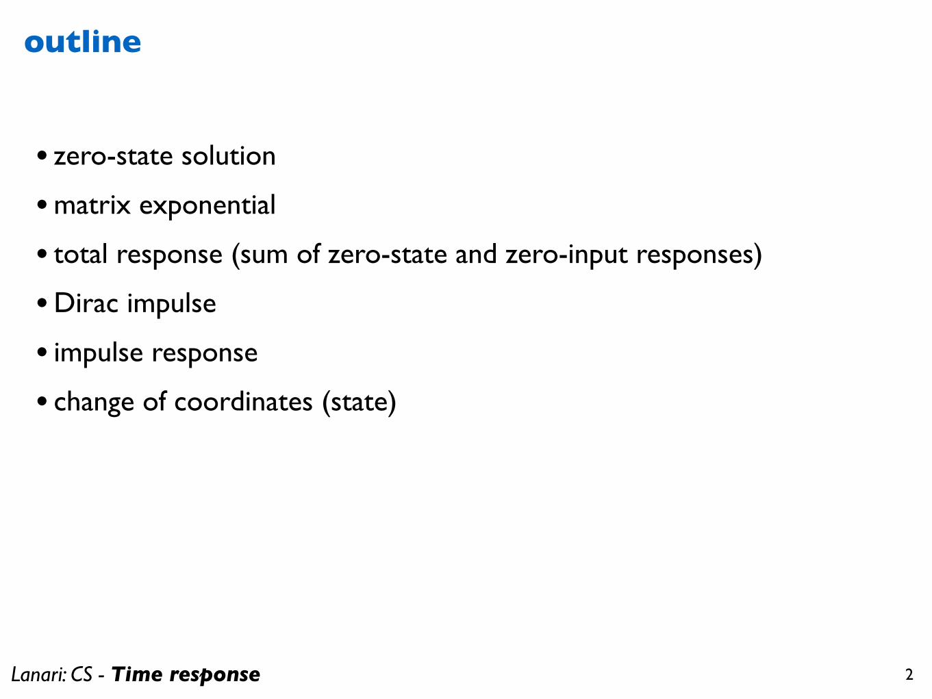
outline
• zero-state solution
• matrix exponential
• total response (sum of zero-state and zero-input responses)
• Dirac impulse
• impulse response
• change of coordinates (state)
Lanari: CS - Time response 3
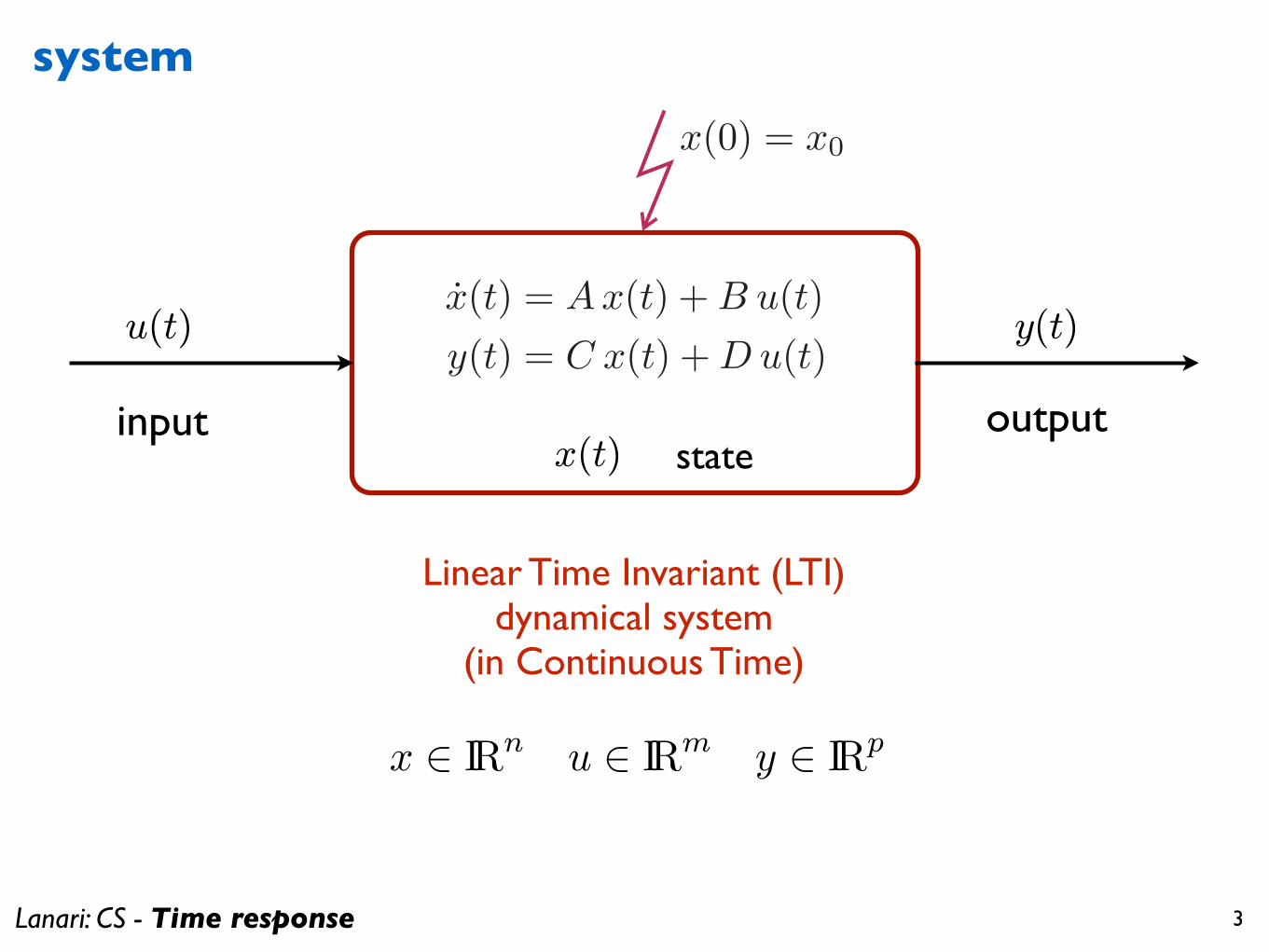
system
Linear Time Invariant (LTI)dynamical system
(in Continuous Time)
1
Kalman Filtering
1.1 Brush-up
dinamica puntomv = F
v = 0
v =F
mv(0) = v0
x(t) = Ax(t) +Bu(t)
y(t) = Cx(t) +Du(t)
x(0) = x0 x ⇥ IRn
x ⇥ IRn u ⇥ IRm y ⇥ IRp
v(t) = v0 +1
m
⇤ t
0F (�)d�
expected value
E(X) = X =
⇤
x�IRnxfX (x)dx
covariancePX = E
�(X � X)(X � X)T
⇥
x(0) = x0
statex(t)
u(t)
input
y(t)
output
x(t) = Ax(t) +B u(t)
y(t) = C x(t) +Du(t)
Lanari: CS - Time response 4
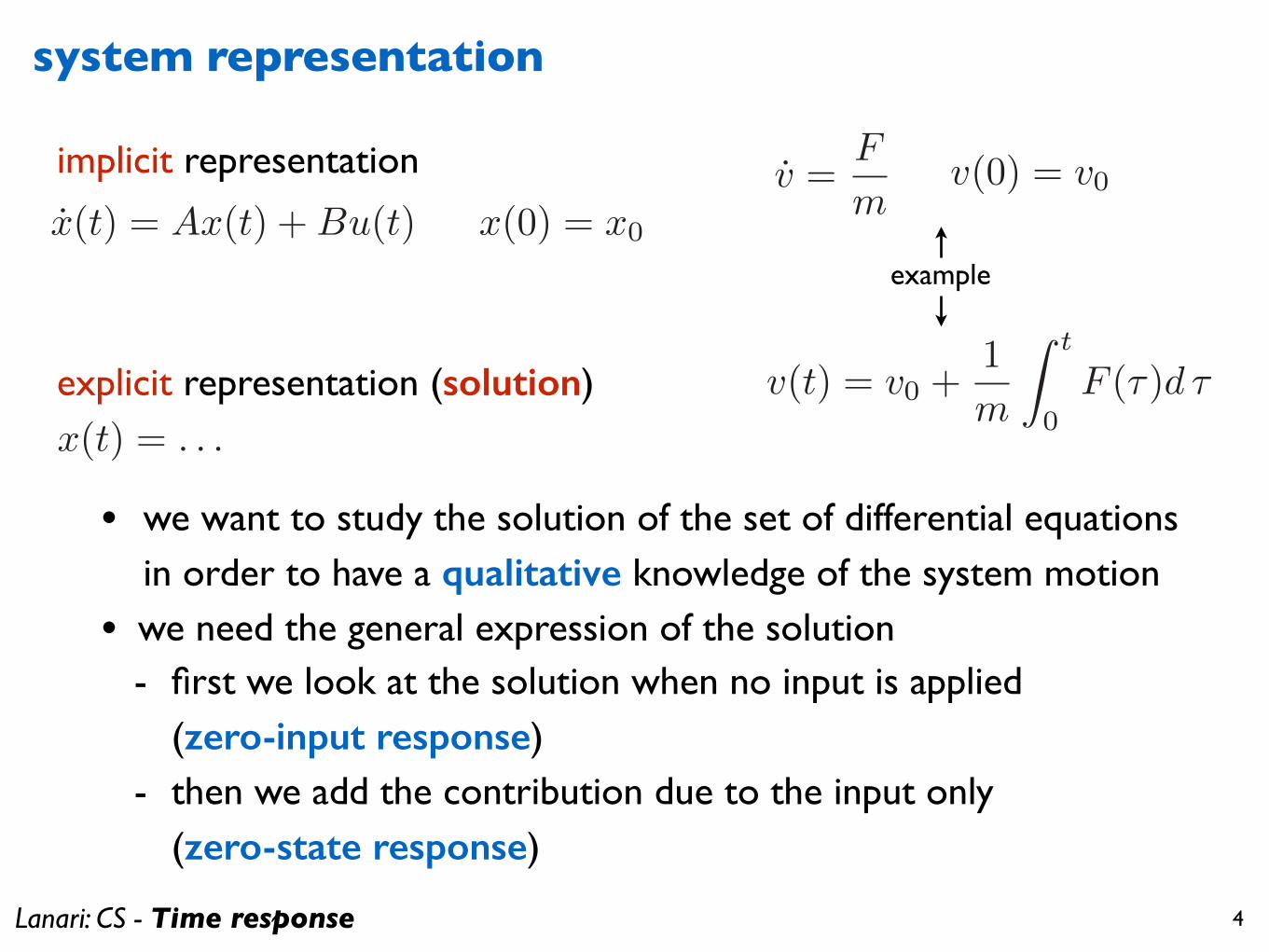
implicit representation
explicit representation (solution)
system representation
example
x(t) = Ax(t) +Bu(t) x(0) = x0
x(t) = . . .
v(t) = v0 +1
m
Z t
0F (⌧)d ⌧
• we want to study the solution of the set of differential equations in order to have a qualitative knowledge of the system motion
• we need the general expression of the solution- first we look at the solution when no input is applied
(zero-input response)- then we add the contribution due to the input only
(zero-state response)
v =F
mv(0) = v0
Lanari: CS - Time response 5
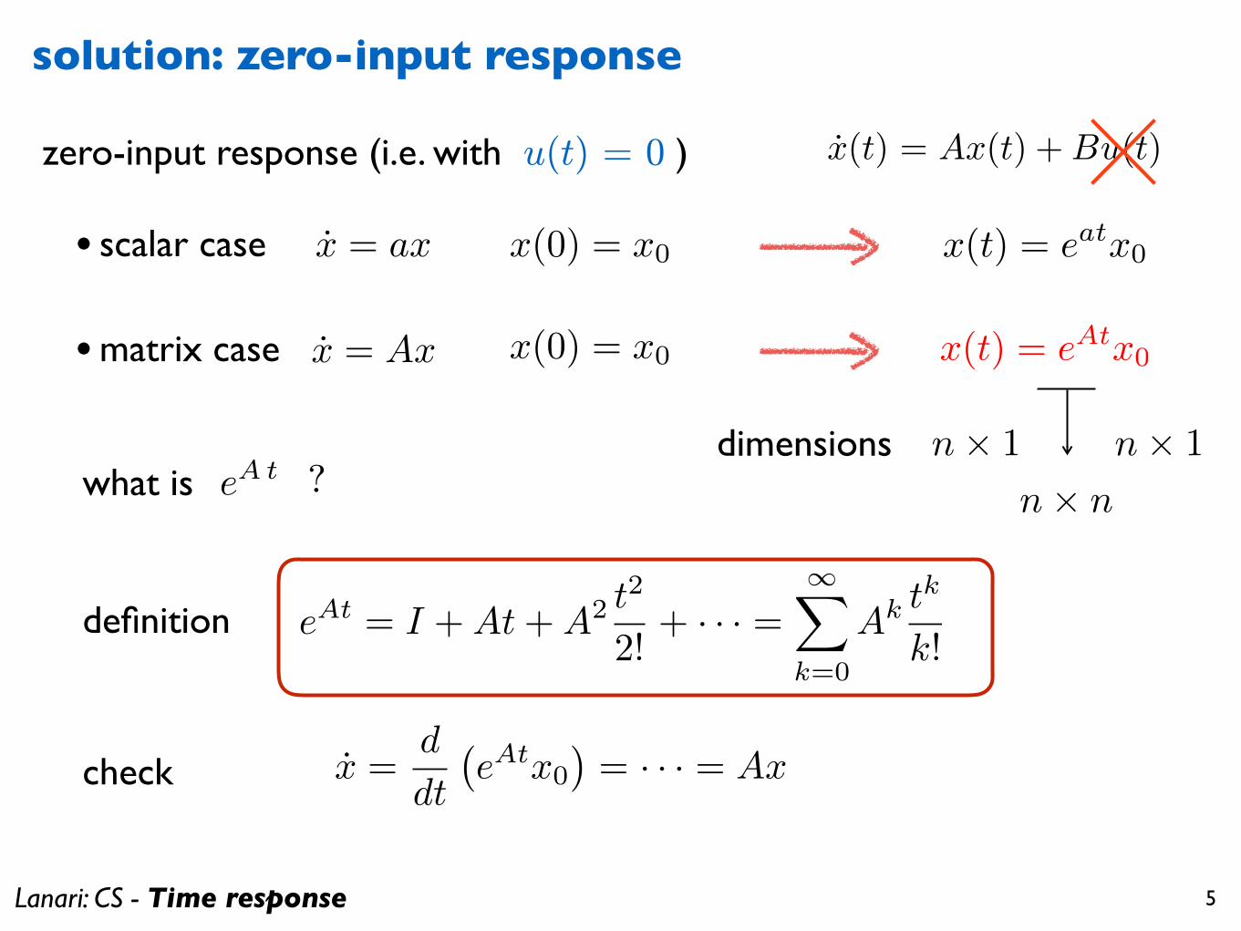
solution: zero-input response
x = ax x(0) = x0• scalar case x(t) = eatx0
zero-input response (i.e. with u(t) = 0 )
1
Kalman Filtering
1.1 Brush-up
dinamica puntomv = F
⇥=
v = 0
v =F
mv(0) = v0
x(t) = Ax(t) +Bu(t)
y(t) = Cx(t) +Du(t)
x(0) = x0 x � IRn
x � IRn u � IRm y � IRp
v(t) = v0 +1
m
� t
0F (�)d�
expected value
E(X) = X =
�
x�IRnxfX (x)dx
• matrix case x = Ax x(0) = x0 x(t) = eAtx0
dimensions n⇥ 1 n⇥ 1
n⇥ n
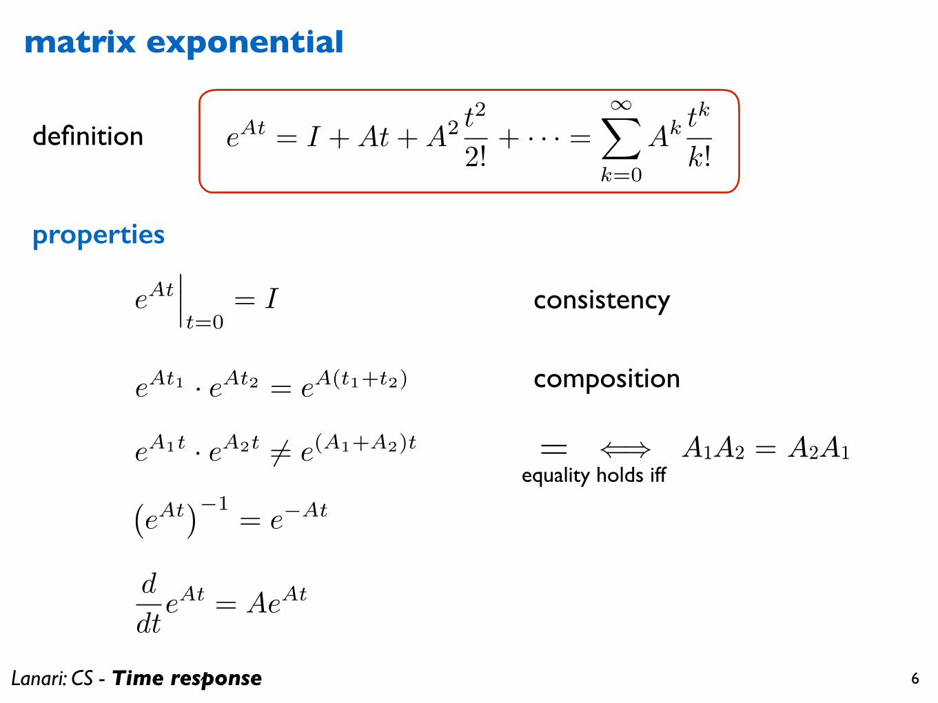
definition eAt = I +At+A2 t2
2!+ · · · =
1X
k=0
Ak tk
k!
check x =d
dt
�eAtx0
�= · · · = Ax
what is<latexit sha1_base64="aw8NiM1JKPHemXSXqbJr7b4fYdc=">AAAB8HicbVBNS8NAEN34WetX1aOXxSJ4kJKIoseKF48V7Ie0sWy2k3bpbhJ2J0IJ/RVePCji1Z/jzX/jts1BWx8MPN6bYWZekEhh0HW/naXlldW19cJGcXNre2e3tLffMHGqOdR5LGPdCpgBKSKoo0AJrUQDU4GEZjC8mfjNJ9BGxNE9jhLwFetHIhScoZUe4DG77pxSHHdLZbfiTkEXiZeTMslR65a+Or2Ypwoi5JIZ0/bcBP2MaRRcwrjYSQ0kjA9ZH9qWRkyB8bPpwWN6bJUeDWNtK0I6VX9PZEwZM1KB7VQMB2bem4j/ee0Uwys/E1GSIkR8tihMJcWYTr6nPaGBoxxZwrgW9lbKB0wzjjajog3Bm395kTTOKt5Fxb07L1ereRwFckiOyAnxyCWpkltSI3XCiSLP5JW8Odp5cd6dj1nrkpPPHJA/cD5/ABWsj+4=</latexit>
eA t ?
Lanari: CS - Time response 6
matrix exponential
eAt = I +At+A2 t2
2!+ · · · =
1X
k=0
Ak tk
k!
eAt���t=0
= I
eAt1 · eAt2 = eA(t1+t2)
eA1t · eA2t �= e(A1+A2)t
�eAt
��1= e�At
d
dteAt = AeAt
()= A1A2 = A2A1
consistency
composition
properties
definition
equality holds iff
Lanari: CS - Time response 7
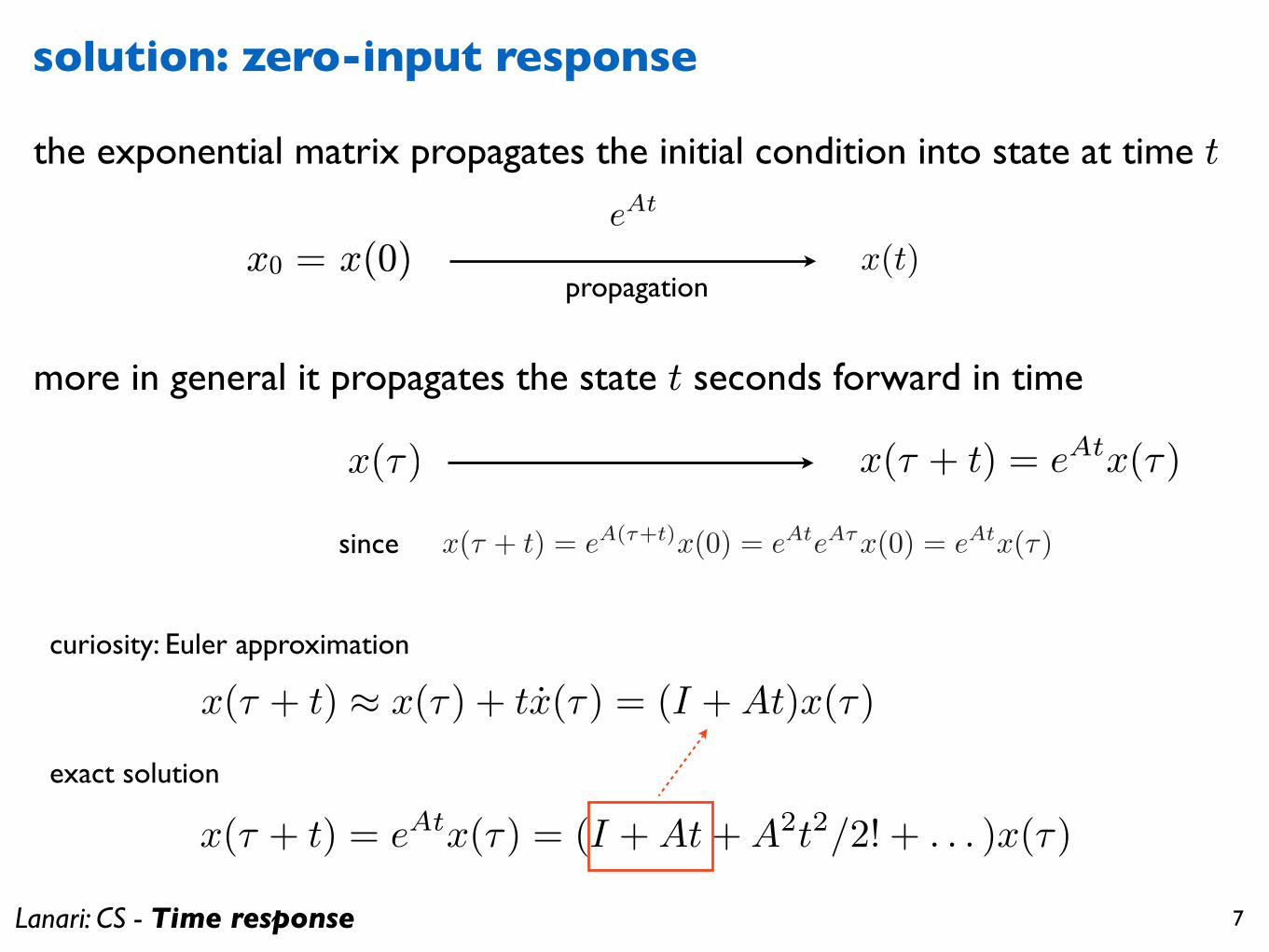
eAt
x(t)propagation
solution: zero-input response
the exponential matrix propagates the initial condition into state at time t
more in general it propagates the state t seconds forward in time
x(� + t) = eAtx(�)
x(� + t) ⇡ x(�) + tx(�) = (I +At)x(�)
x(� + t) = eAtx(�) = (I +At+A2t2/2! + . . . )x(�)
x(�)
curiosity: Euler approximation
exact solution
x(⌧ + t) = eA(⌧+t)x(0) = eAteA⌧x(0) = eAtx(⌧)since
x0 = x(0)
Lanari: CS - Time response 8
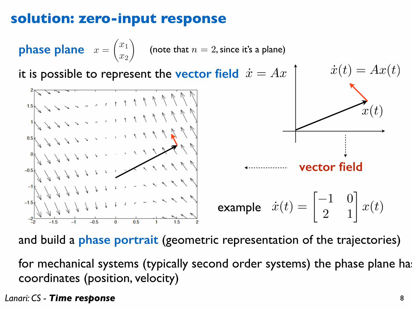
solution: zero-input response
x = Ax
phase plane
x(t)
x(t) = Ax(t)
vector field
x(t) =
�1 02 1
�x(t)
x =
✓x1
x2
◆
it is possible to represent the vector field
and build a phase portrait (geometric representation of the trajectories)
(note that n = 2, since it’s a plane)
example
for mechanical systems (typically second order systems) the phase plane has coordinates (position, velocity)
Lanari: CS - Time response 9
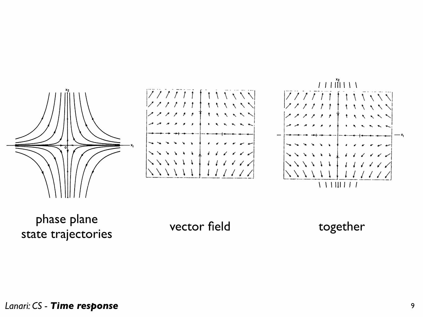
phase planestate trajectories vector field together
Lanari: CS - Time response 10
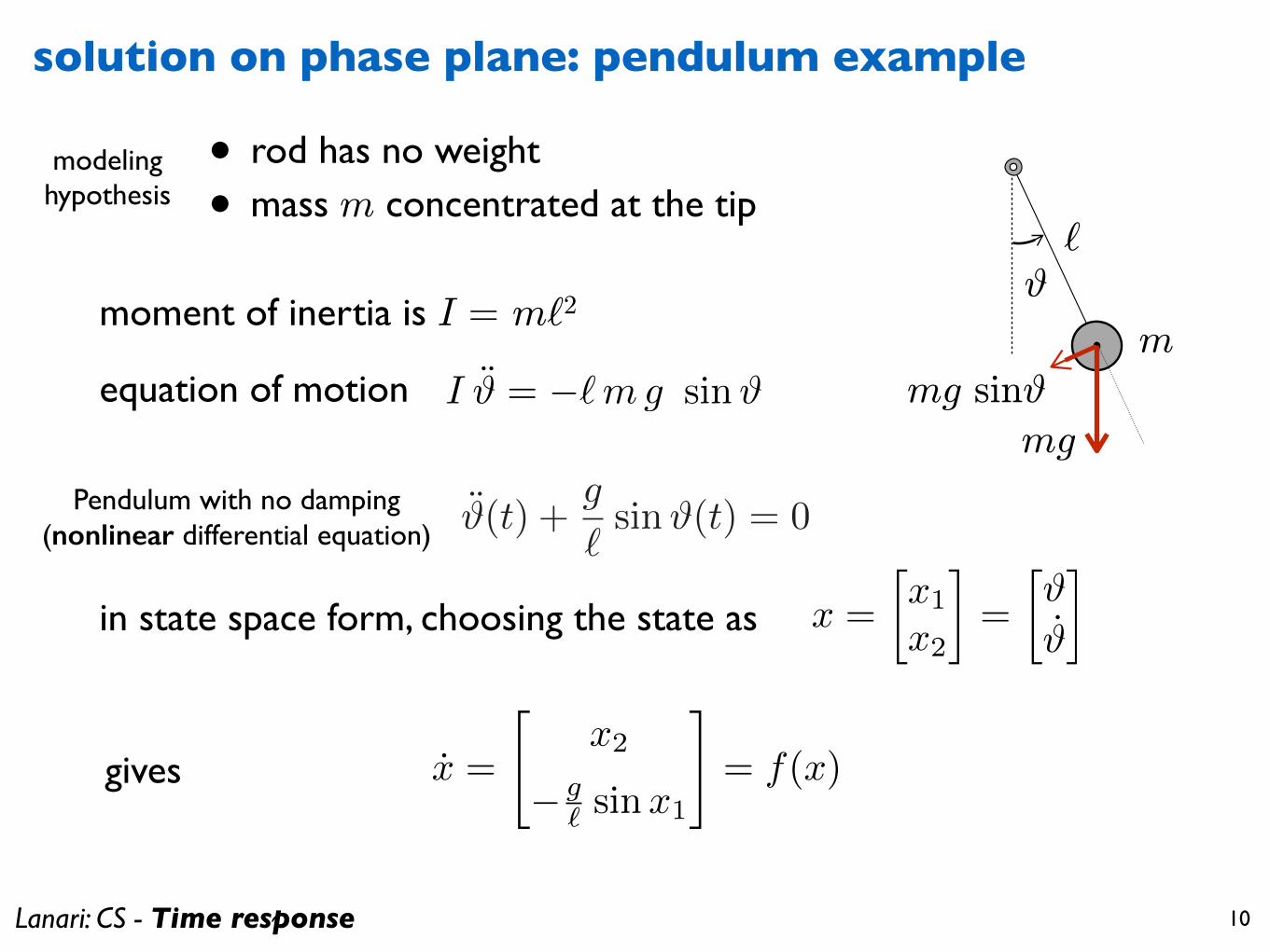
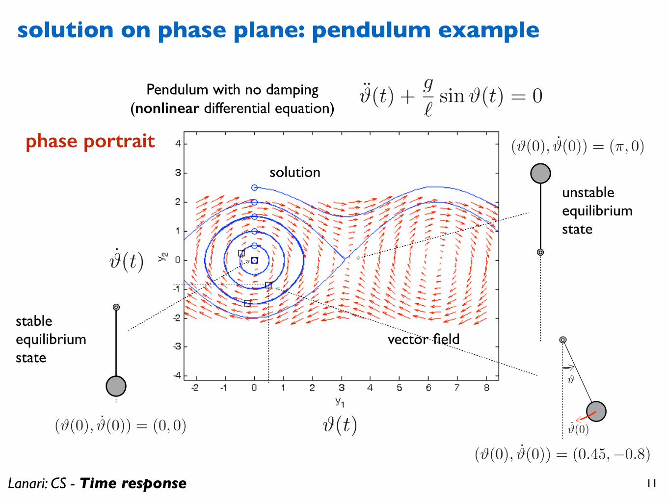
solution on phase plane: pendulum example
Pendulum with no damping (nonlinear differential equation) #(t) +
g
`sin#(t) = 0
modelinghypothesis
• rod has no weight
• mass m concentrated at the tip
moment of inertia is I = m`2
`
m
#
m g sin #
m g
<latexit sha1_base64="sscXejmbQjMXopY+GrtoO3DJ3bk=">AAACJHicbVDLSgMxFM34tr6qLt0Ei+BCy4woCiIU3OhOwarQGUomc6cNZjJDcqdQSj/Gjb/ixoUPXLjxW8zUgtp6ScLhnHOT3BNmUhh03Q9nYnJqemZ2br60sLi0vFJeXbs2aa451HkqU30bMgNSKKijQAm3mQaWhBJuwrvTQr/pgDYiVVfYzSBIWEuJWHCGlmqWj8+pv0P9KEqR+h2msQ3I6AndpT5IWWhJcbQKk11GqB9bs1xxq+6g6DjwhqBChnXRLL/6UcrzBBRyyYxpeG6GQc9eJ7iEfsnPDWSM37EWNCxULAET9AZD9umWZSIap9puhXTA/u7oscSYbhJaZ8KwbUa1gvxPa+QYHwU9obIcQfHvh+JcUkxpkRiNhAaOsmsB41rYv1LeZppxtLmWbAje6Mjj4Hqv6h1U3cv9Sq02jGOObJBNsk08ckhq5IxckDrh5J48kmfy4jw4T86b8/5tnXCGPevkTzmfXz7GoYY=</latexit>
I # = �`mg sin#equation of motion
gives
<latexit sha1_base64="Lt19X/Itg9cW8GyD5uiV1eQj93k=">AAACUXicbVFNSwMxEJ2u360fVY9egkXwVHZF0YtQ8OJRwarQLSWbTtvQbHZJZkvL0r/oQU/+Dy8eFNNasFoHQh7vzZskL1GqpCXffy14S8srq2vrG8XS5tb2Tnl3794mmRFYF4lKzGPELSqpsU6SFD6mBnkcKXyI+lcT/WGAxspE39EoxWbMu1p2pODkqFa5N2SXLIywK3UexZyMHI7ZsBWwMHTbCQtRt3+ExdZwwA31kPjEELYTmmfmva1yxa/602KLIJiBCszqplV+duNEFqMmobi1jcBPqZm74VIoHBfDzGLKRZ93seGg5jHaZj5NZMyOHNNmncS4pYlN2XlHzmNrR3HkOt39evavNiH/0xoZdS6audRpRqjF90GdTDFK2CRe1pYGBamRA1wY6e7KRI8bLsh9QtGFEPx98iK4P6kGZ1X/9rRSq83iWIcDOIRjCOAcanANN1AHAU/wBh/wWXgpvHvged+tXmHm2Ydf5ZW+AOIStJA=</latexit>
x =
x1
x2
�=
##
�
<latexit sha1_base64="4zv1QMFzvKEZUNv6hPhlSiPd+/Y=">AAACO3icbVA9SwNBEN3z2/gVtbQZDIIWhrugaCMEbCxVjArZEPY2c3Fxb+/Y3ZOE4/6XjX/CzsbGQhFbezcx4OeDgcebN8zMC1MpjPX9B29sfGJyanpmtjQ3v7C4VF5eOTdJpjk2eCITfRkyg1IobFhhJV6mGlkcSrwIrw8H/Ysb1EYk6sz2U2zFrKtEJDizTmqXT2knsdCDA6AhdoXKw5hZLXoF9No1oLS5m9oWbNNIM553i5yilAVQI5QzBEBRdb5GDiDa7G21yxW/6g8Bf0kwIhUywnG7fO+O4FmMynLJjGkGvluaM20Fl1iUaGYwZfyadbHpqGIxmlY+/L2ADad0IEq0K2VhqH6fyFlsTD8OndOdeWV+9wbif71mZqP9Vi5UmllU/HNRlEmwCQyChI7QyK3sO8K4Fu5W4FfMxWRd3CUXQvD75b/kvFYNdqv+yU6lXh/FMUPWyDrZJAHZI3VyRI5Jg3BySx7JM3nx7rwn79V7+7SOeaOZVfID3vsHiRStLA==</latexit>
x =
"x2
� g` sinx1
#= f(x)
in state space form, choosing the state as
Lanari: CS - Time response 11
solution on phase plane: pendulum example
solution
vector field
Pendulum with no damping (nonlinear differential equation)
#(t)
#(t)
#(t) +g
`sin#(t) = 0
(#(0), #(0)) = (0, 0)
(#(0), #(0)) = (⇡, 0)
unstableequilibriumstate
stableequilibriumstate
(#(0), #(0)) = (0.45,�0.8)
#
#(0)
phase portrait
Lanari: CS - Time response 12
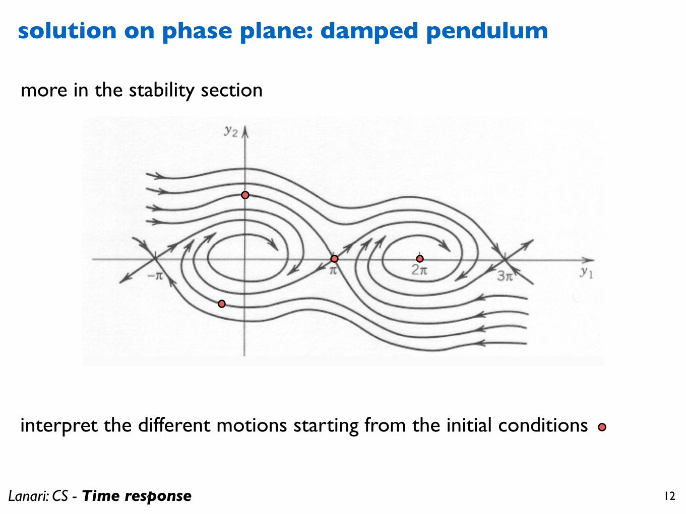
solution on phase plane: damped pendulum
more in the stability section
interpret the different motions starting from the initial conditions

Lanari: CS - Time response 13
solution: total response
scalar case
x = ax+ bu x(t) = eatx0 +
Z t
0ea(t��)bu(�)d�
check using theLeibniz integral rule
d
dt
Z t
0f(t, �)d� =
Z t
0
d
dtf(t, �)d� + f(t, �)
���=t
x = aeatx0 +
Z t
0aea(t��)bu(�)d� + bu(t) = ax+ bu
solution is
example: see the point mass v(t) = v0 +1
m
Z t
0F (⌧)d⌧
definition: convolution integral
<latexit sha1_base64="Us2oHPS/2b+Q9IzGk+S8Q4N2BgE=">AAACG3icbVDLSgMxFM3UV62vqks3wSK0C8tMUXQjFNy4rGAf0BlLJs20oZnMkNwRytD/cOOvuHGhiCvBhX9jpu1CWw+EezjnXm7u8WPBNdj2t5VbWV1b38hvFra2d3b3ivsHLR0lirImjUSkOj7RTHDJmsBBsE6sGAl9wdr+6Drz2w9MaR7JOxjHzAvJQPKAUwJG6hVrQRkq2NVAFB5k9Aq7XELPvgdsrFMXSFIxzqz2s9IrluyqPQVeJs6clNAcjV7x0+1HNAmZBCqI1l3HjsFLiQJOBZsU3ESzmNARGbCuoZKETHvp9LYJPjFKHweRMk8Cnqq/J1ISaj0OfdMZEhjqRS8T//O6CQSXXsplnACTdLYoSASGCGdB4T5XjIIYG0Ko4uavmA6JIhRMnAUTgrN48jJp1arOedW+PSvV6/M48ugIHaMyctAFqqMb1EBNRNEjekav6M16sl6sd+tj1pqz5jOH6A+srx94O56Z</latexit>
f(t) ? g(t) =
Z t
0f(t� ⌧)g(⌧)d⌧

Lanari: CS - Time response 14
solution: total response
matrix case
x(t) = eAtx0 +
Z t
0eA(t��)Bu(�)d�
zero-input response (ZIR)
eAt state-transition matrix
zero-state response (ZSR)
y(t) = CeAtx0 +
Z t
0CeA(t��)Bu(�)d� +Du(t)
CeAt output-transition matrix
N.B. product is not commutative for matrices
state
output
Lanari: CS - Time response 15
solution: total response
total response = zero-input response + zero-state response
u(t) = 0
x(0) 6= 0 x(0) = 0
u(t) 6= 0
two distinct contributions to the motion of a linear system
• a non-zero initial condition causes motion as well as
• a non-zero input
alternative names
• zero-input response = free response/evolution
• zero-state response = forced response/evolution
Lanari: CS - Time response 16
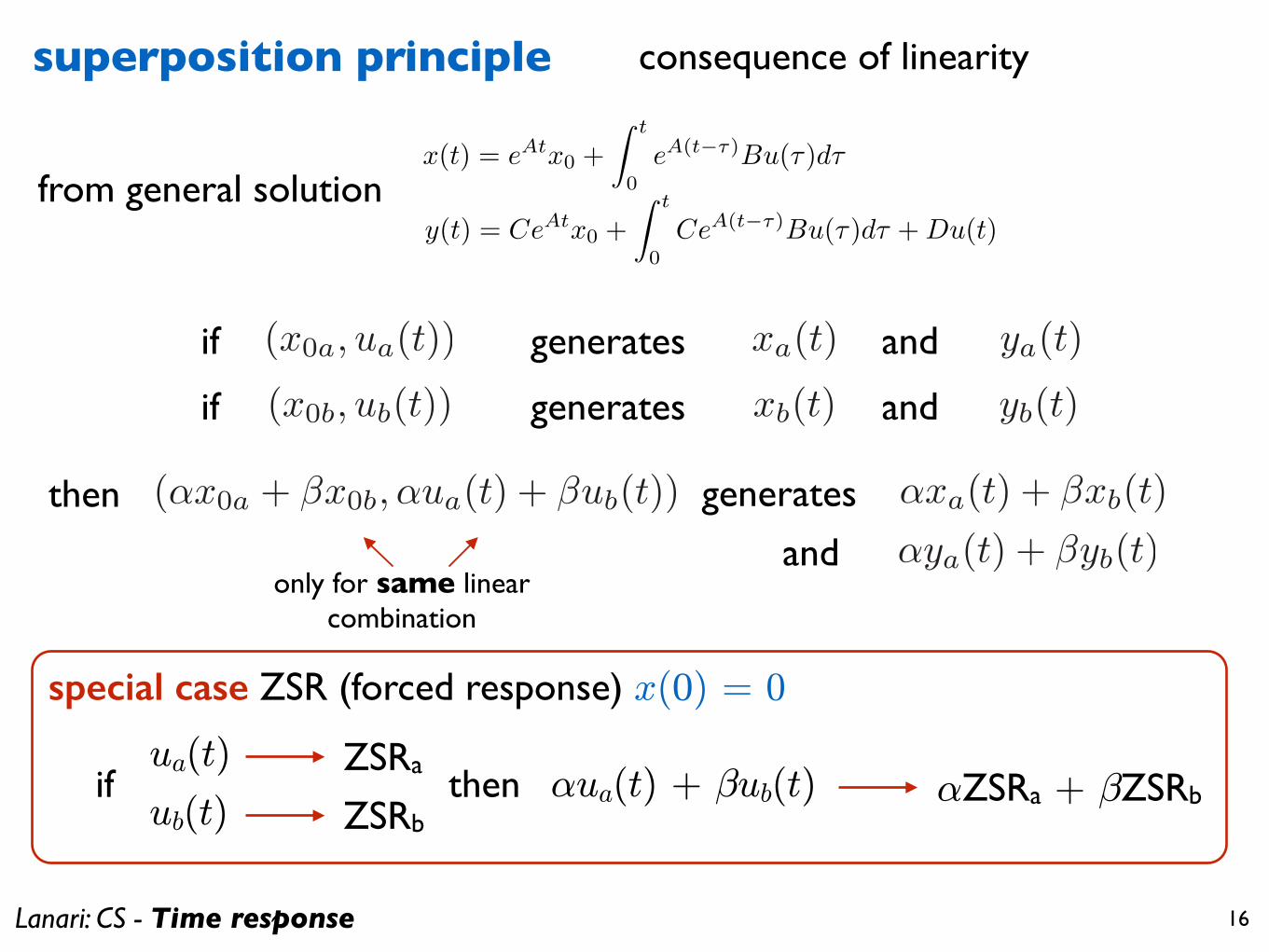
superposition principle
x(t) = eAtx0 +
Z t
0eA(t��)Bu(�)d�
y(t) = CeAtx0 +
Z t
0CeA(t��)Bu(�)d� +Du(t)
only for same linearcombination
(x0a, ua(t))
(x0b, ub(t))
xa(t)
xb(t)
(↵x0a + �x0b,↵ua(t) + �ub(t)) ↵xa(t) + �xb(t)
if generates
if generates
then generates
and
and
↵ya(t) + �yb(t)
ya(t)
yb(t)
and
from general solution
special case ZSR (forced response) x(0) = 0
ua(t)
ub(t)if
ZSRa
ZSRbthen ®ua(t) + ¯ub(t) ®ZSRa + ¯ZSRb
consequence of linearity
Lanari: CS - Time response 17
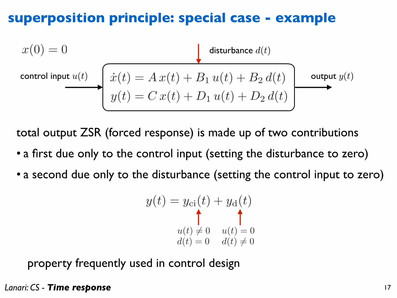
superposition principle: special case - example
disturbance d(t)
x(t) = Ax(t) +B1 u(t) +B2 d(t)
y(t) = C x(t) +D1 u(t) +D2 d(t)
control input u(t) output y(t)
x(0) = 0
y(t) = yci(t) + yd(t)
total output ZSR (forced response) is made up of two contributions
• a first due only to the control input (setting the disturbance to zero)
• a second due only to the disturbance (setting the control input to zero)
u(t) 6= 0d(t) = 0
u(t) = 0d(t) 6= 0
property frequently used in control design
Lanari: CS - Time response 18
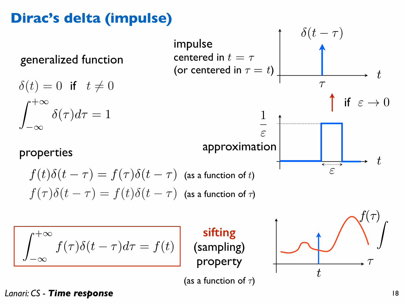
Dirac’s delta (impulse)
generalized functiont
�(t� ⇥)
⌧Z +1
�1�(⇥)d⇥ = 1
Z +1
�1f(⇥)�(t� ⇥)d⇥ = f(t)
sifting (sampling)property
t"
1
"
" ! 0
approximation
f(t)�(t� ⇥) = f(⇥)�(t� ⇥)
t⌧
f(¿)Z
properties
(as a function of t)
(as a function of ¿)
if�(t) = 0 t 6= 0
impulse centered in t = ¿ (or centered in ¿ = t)
if
f(⌧)�(t� ⌧) = f(t)�(t� ⌧) (as a function of ¿)
Lanari: CS - Time response 19
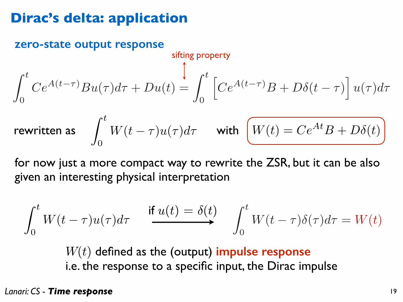
Dirac’s delta: application
Z t
0W (t� �)u(�)d� W (t) = CeAtB +D�(t)with
sifting property
rewritten as
Z t
0W (t� �)u(�)d�
W(t) defined as the (output) impulse response i.e. the response to a specific input, the Dirac impulse
zero-state output response
Z t
0CeA(t�⌧)Bu(⌧)d⌧ +Du(t) =
Z t
0
hCeA(t�⌧)B +D�(t� ⌧)
iu(⌧)d⌧
Z t
0W (t� ⌧)�(⌧)d⌧ = W (t)
for now just a more compact way to rewrite the ZSR, but it can be also given an interesting physical interpretation
if u(t) = ±(t)
Lanari: CS - Time response 20
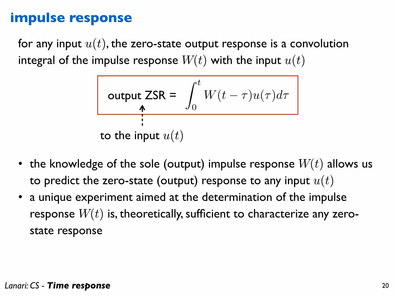
for any input u(t), the zero-state output response is a convolution integral of the impulse response W(t) with the input u(t)
Z t
0W (t� �)u(�)d�
impulse response
output ZSR =
to the input u(t)
• the knowledge of the sole (output) impulse response W(t) allows us to predict the zero-state (output) response to any input u(t)
• a unique experiment aimed at the determination of the impulse response W(t) is, theoretically, sufficient to characterize any zero-state response
Lanari: CS - Time response 21
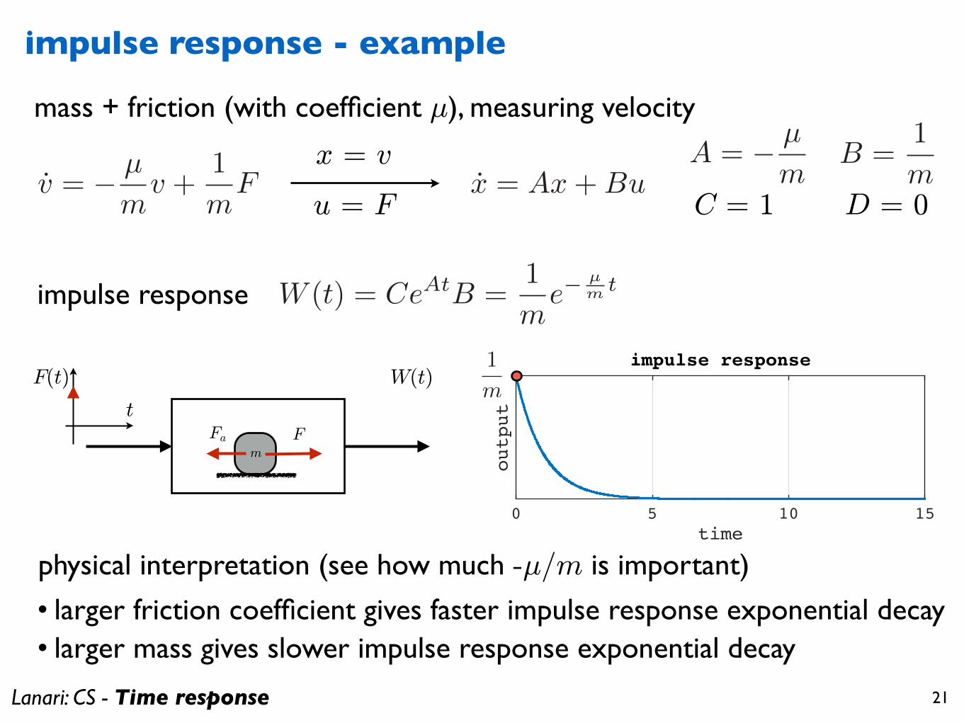
impulse response - example
mass + friction (with coefficient µ), measuring velocity
v = � µ
mv +
1
mF
W (t) = CeAtB =1
me�
µm t
x = Ax+BuA = � µ
mB =
1
mC = 1 D = 0
impulse response
x = v
u = F
m
FFa
t
F(t) W(t)
time0 5 10 15
output
impulse response1
m
• larger friction coefficient gives faster impulse response exponential decay• larger mass gives slower impulse response exponential decay
physical interpretation (see how much -µ/m is important)
Lanari: CS - Time response 22
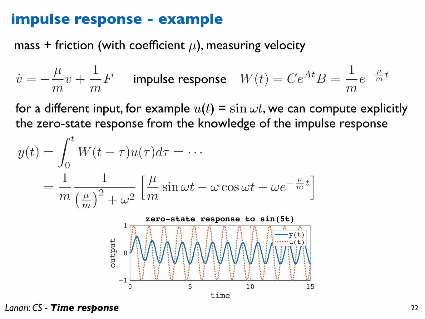
impulse response - example
mass + friction (with coefficient µ), measuring velocity
v = � µ
mv +
1
mF W (t) = CeAtB =
1
me�
µm t
y(t) =
Z t
0W (t� ⌧)u(⌧)d⌧ = · · ·
=1
m
1� µm
�2+ !2
h µm
sin!t� ! cos!t+ !e�µm t
i
impulse response
for a different input, for example u(t) = sin !t, we can compute explicitly the zero-state response from the knowledge of the impulse response
time0 5 10 15
output
-1
0
1zero-state response to sin(5t)
y(t)u(t)
Lanari: CS - Time response 23
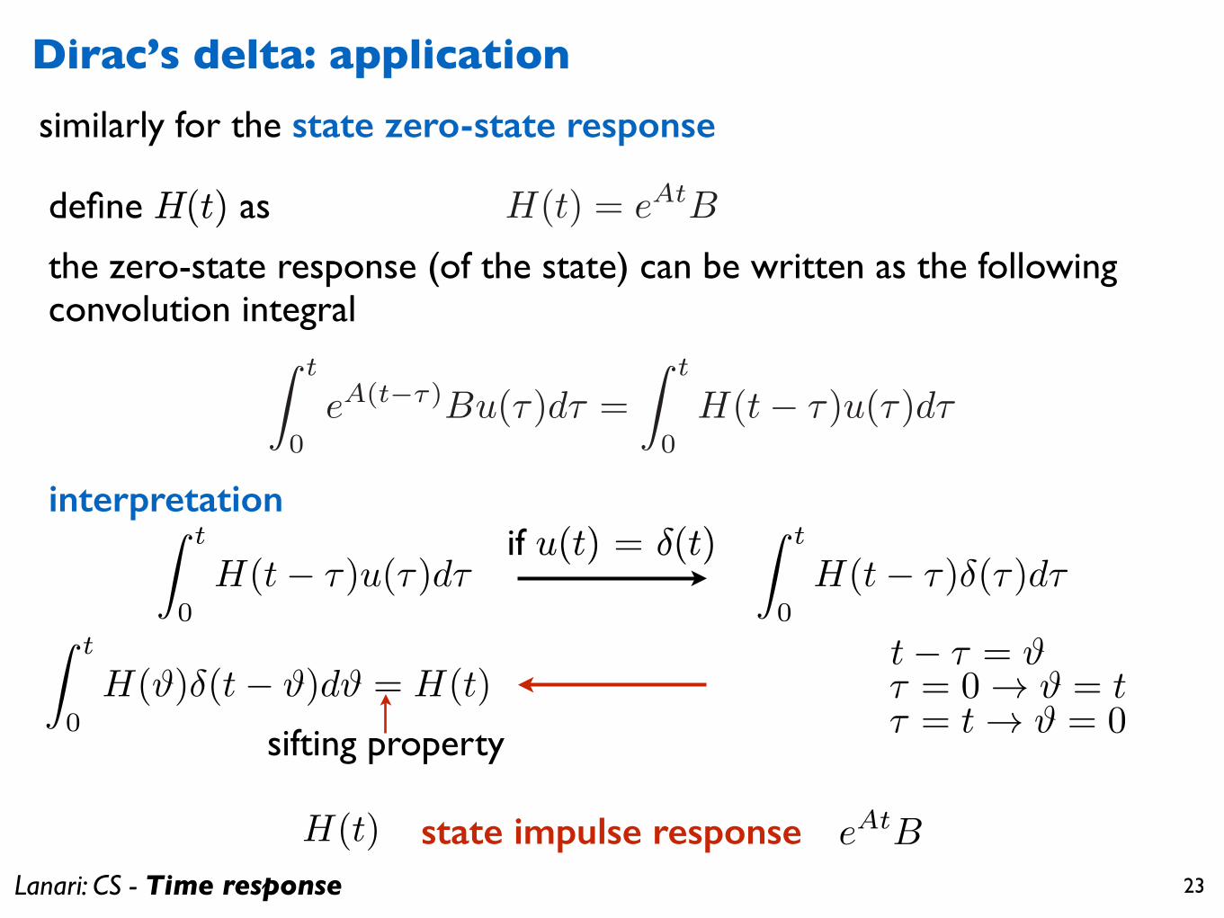
Dirac’s delta: applicationsimilarly for the state zero-state response
H(t) = eAtBdefine H(t) as
the zero-state response (of the state) can be written as the following convolution integral
Z t
0eA(t�⌧)
Bu(⌧)d⌧ =
Z t
0H(t� ⌧)u(⌧)d⌧
Z t
0H(t� �)u(�)d�
Z t
0H(t� ⇥)�(⇥)d⇥
t� � = ⇥� = 0 ! ⇥ = t� = t ! ⇥ = 0
Z t
0H(⇥)�(t� ⇥)d⇥ = H(t)
sifting property
H(t) state impulse response eAtB
if u(t) = ±(t)interpretation
Lanari: CS - Time response 24
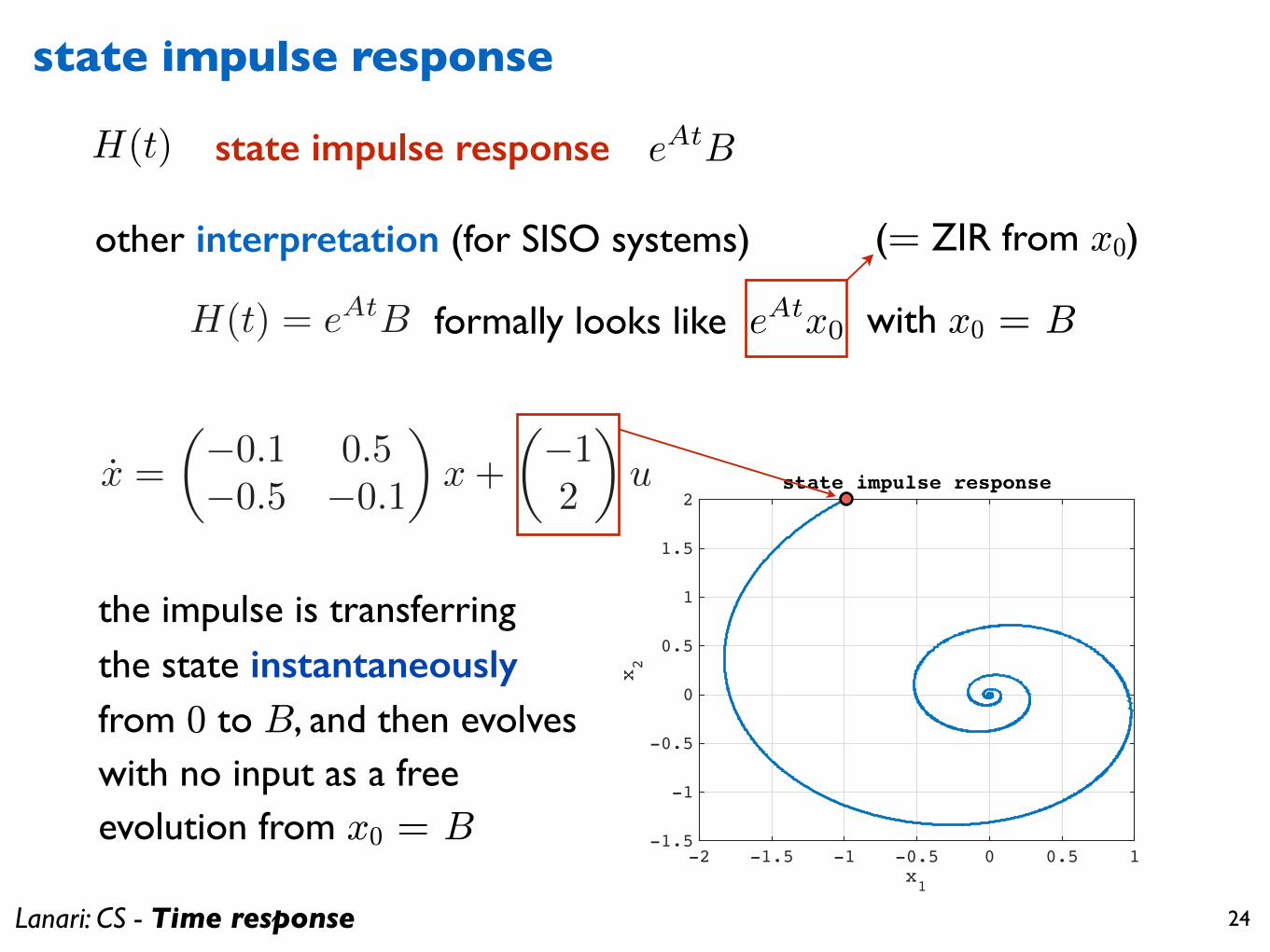
state impulse response
H(t) state impulse response eAtB
eAtx0
the impulse is transferringthe state instantaneously from 0 to B, and then evolves with no input as a free evolution from x0 = B
(= ZIR from x0)
formally looks likeH(t) = eAtB with x0 = B
other interpretation (for SISO systems)
x1-2 -1.5 -1 -0.5 0 0.5 1
x 2
-1.5
-1
-0.5
0
0.5
1
1.5
2state impulse responsex =
✓�0.1 0.5�0.5 �0.1
◆x+
✓�12
◆u
Lanari: CS - Time response 25
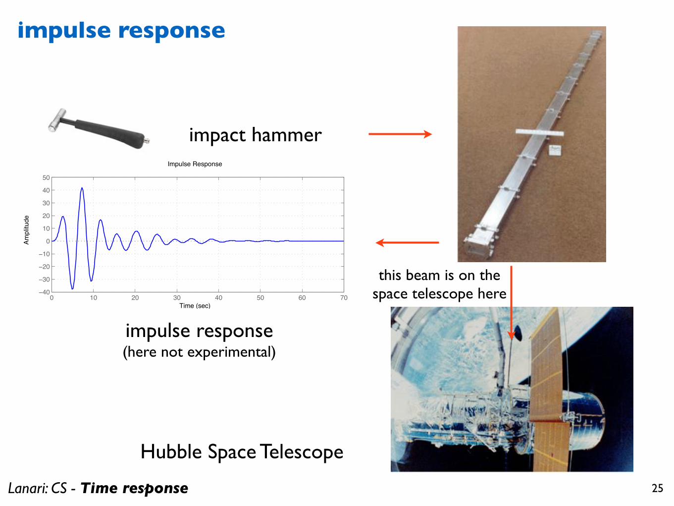
impulse response
impact hammer
0 10 20 30 40 50 60 70�40
�30
�20
�10
0
10
20
30
40
50
Impulse Response
Time (sec)
Ampl
itude
Hubble Space Telescope
impulse response(here not experimental)
this beam is on the space telescope here
Lanari: CS - Time response 26
impulse response: experimental determination
Modal testing for vibration analysis: • the impulse, which has an infinitely small duration, is the ideal testing
impact to a structure: all vibration modes will be excited with the same amount of energy (more on this in the frequency analysis section)
• the impact hammer should be able to replicate this ideal impulse but in reality the strike cannot have an infinitesimal small duration
• the finite duration of the real impact influences the frequency content of the applied force: the longer is the duration the smaller bandwidth
more in the “Mechanical Vibrations” course
Lanari: CS - Time response 27
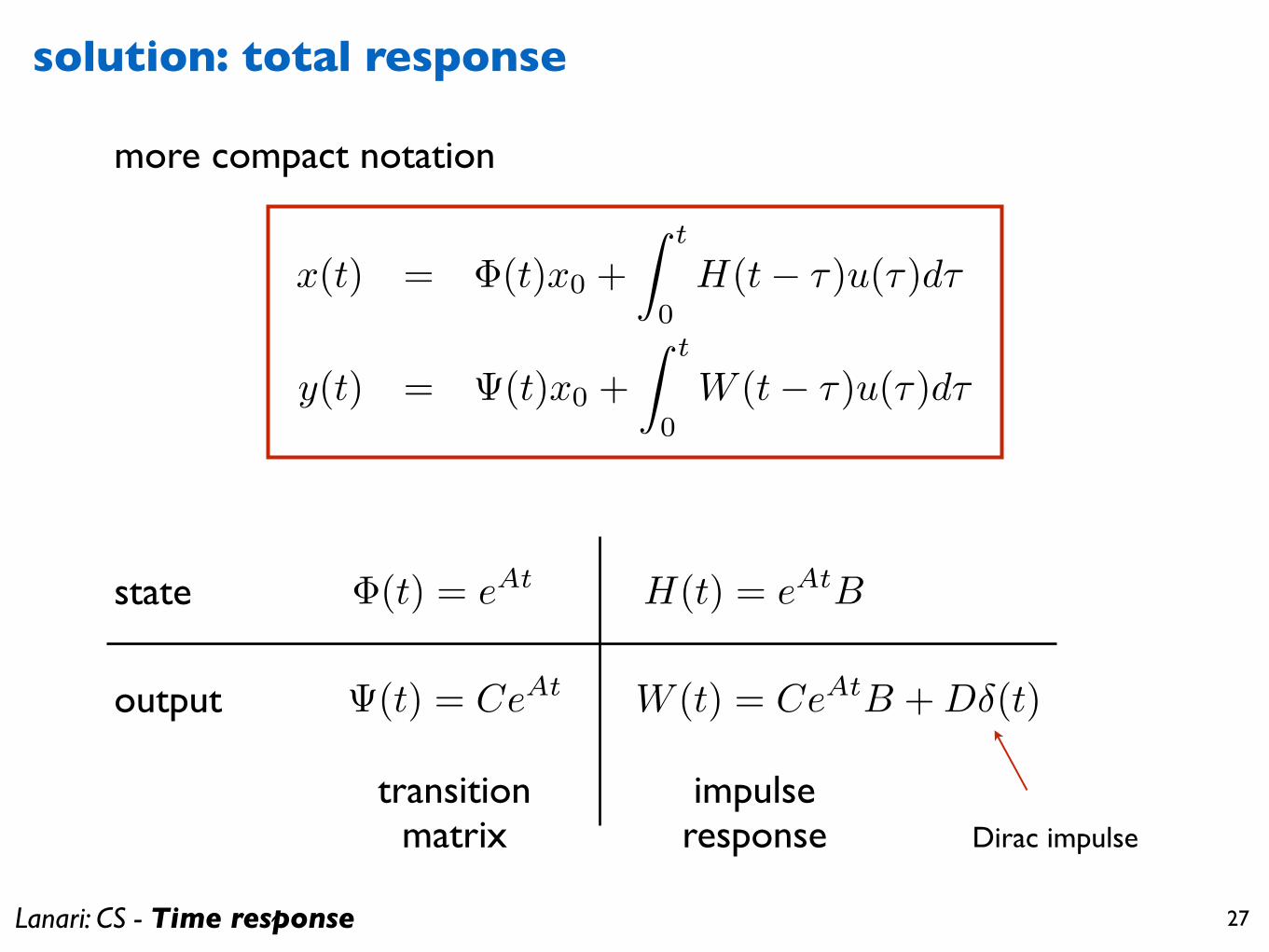
solution: total response
x(t) = �(t)x0 +
Z t
0H(t� �)u(�)d�
y(t) = ⇥(t)x0 +
Z t
0W (t� �)u(�)d�
�(t) = eAtH(t) = e
AtB
�(t) = CeAt W (t) = CeAtB +D�(t)
state
output
transitionmatrix
impulseresponse Dirac impulse
more compact notation

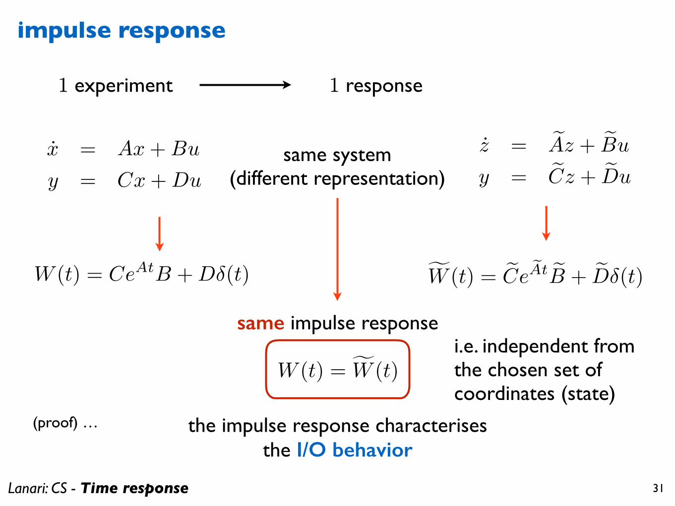
Lanari: CS - Time response 28
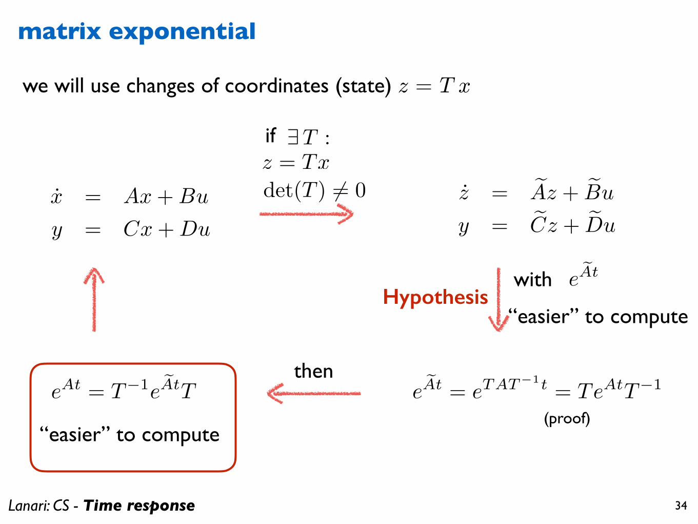
change of coordinates
z = eAz + eBu
y = eCz + eDux = Ax+Bu
y = Cx+Du
(A,B,C,D) ( eA, eB, eC, eD)z = Tx det(T ) 6= 0
same system
eA = T AT�1 eB = T B eC = C T�1 eD = D
equivalent system representation (proof) …
input u & output y do not change, only state is chosen differently
state space representation
state x state z
change of coordinates
the matrices of the two equivalent system representations are related as
Lanari: CS - Time response 29
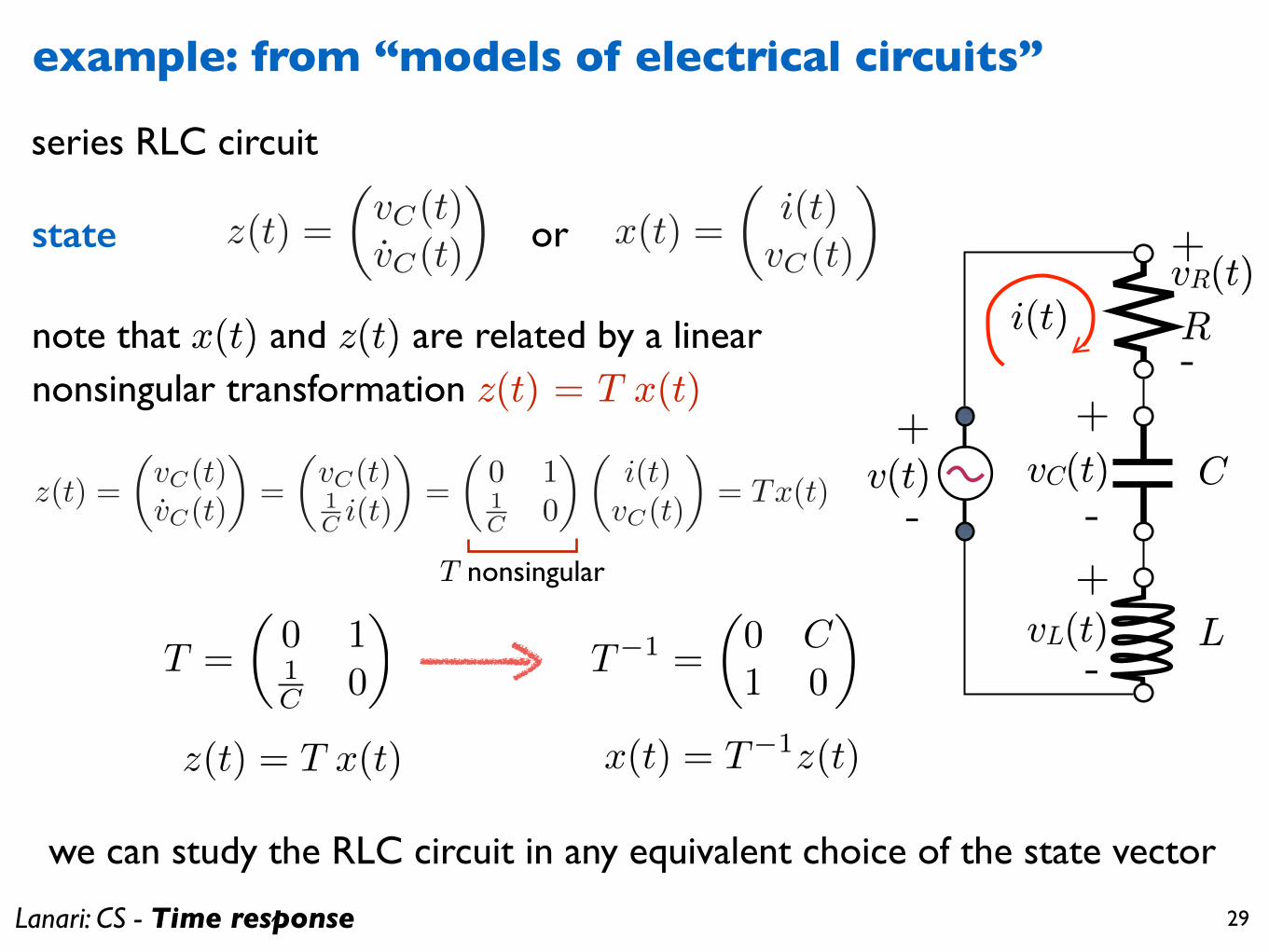
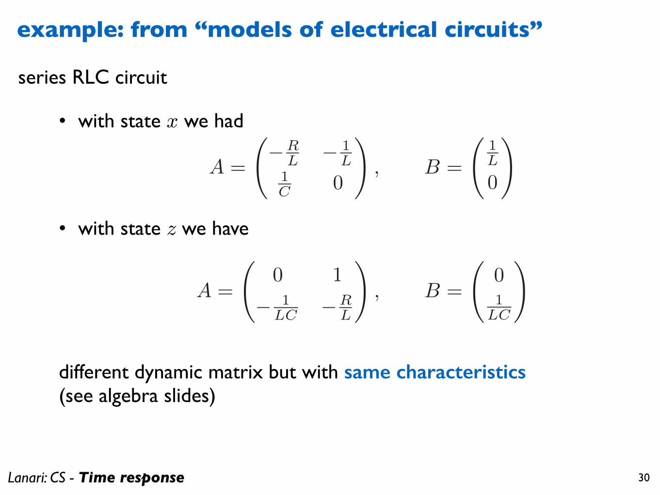
series RLC circuit
or
example: from “models of electrical circuits”
z(t) =
✓vC(t)vC(t)
◆x(t) =
✓i(t)vC(t)
◆state
+
-
i(t) R
L
CvC(t)v(t)+
-
+
-vL(t)
vR(t)+
-note that x(t) and z(t) are related by a linear nonsingular transformation z(t) = T x(t)
z(t) =
✓vC(t)vC(t)
◆=
✓vC(t)1C i(t)
◆=
✓0 11C 0
◆✓i(t)vC(t)
◆= Tx(t)
T nonsingular<latexit sha1_base64="/74e169KKo6dh/3aOPlBUPgPe1Y=">AAACJHicbVDLSgMxFM3UVx1fVZdugkVxVWZEURCh0I3LCn1Bp5RMeqcNzWSGJCOWYT7Gjb/ixoUPXLjxW0wfiLYeCBzOOZfce/yYM6Ud59PKLS2vrK7l1+2Nza3tncLuXkNFiaRQpxGPZMsnCjgTUNdMc2jFEkjoc2j6w8rYb96BVCwSNT2KoROSvmABo0QbqVu4su0avsaeD30m0jgkWrL7zMHH2MWeh71AEpq6WVrJjOR4IHo/IbtbKDolZwK8SNwZKaIZqt3Cm9eLaBKC0JQTpdquE+tOSqRmlENme4mCmNAh6UPbUEFCUJ10cmSGj4zSw0EkzRMaT9TfEykJlRqFvkmaBQdq3huL/3ntRAeXnZSJONEg6PSjIOFYR3jcGO4xCVTzkSGESmZ2xXRATC/a9DouwZ0/eZE0Tkvuecm5PSuWy7M68ugAHaIT5KILVEY3qIrqiKIH9IRe0Kv1aD1b79bHNJqzZjP76A+sr2/V9aKJ</latexit>
T =
✓0 11C 0
◆ <latexit sha1_base64="uqJKnDcyGtoW48uFR/j2pc0Fo4s=">AAACIHicbZDLSgMxFIYz9VbH26hLN8GiuLHMiFI3QqEblxV6g04tmfS0Dc1khiQjlqGP4sZXceNCEd3p05heEG09EPj4/3PIOX8Qc6a0635amaXlldW17Lq9sbm1vePs7tVUlEgKVRrxSDYCooAzAVXNNIdGLIGEAYd6MCiN/fodSMUiUdHDGFoh6QnWZZRoI7Wdgm1XbtNTb4SvMPYD6DGRxiHRkt2PXHyMS9j3sWfAxT6Izo/XdnJu3p0UXgRvBjk0q3Lb+fA7EU1CEJpyolTTc2PdSonUjHIY2X6iICZ0QHrQNChICKqVTg4c4SOjdHA3kuYJjSfq74mUhEoNw8B0mv36at4bi/95zUR3L1spE3GiQdDpR92EYx3hcVq4wyRQzYcGCJXM7Ippn0hCtcnUNiF48ycvQu0s713k3ZvzXLE4iyOLDtAhOkEeKqAiukZlVEUUPaAn9IJerUfr2Xqz3qetGWs2s4/+lPX1DY+EoDI=</latexit>
T�1 =
✓0 C1 0
◆
<latexit sha1_base64="ZJTSW/WV7pYFd6ZPOQkEjdp2H4o=">AAAB/nicbVDLSgMxFL1TX3V8jYorN8Ei1IVlRhTdCAU3Liv0Be1YMmnahmYyQ5IR61DwV9y4UMSt3+HOvzFtZ6HVAxdOzrmX3HuCmDOlXffLyi0sLi2v5FfttfWNzS1ne6euokQSWiMRj2QzwIpyJmhNM81pM5YUhwGnjWB4NfEbd1QqFomqHsXUD3FfsB4jWBup4+zZ9j0q6iN0iaq36bE3Rg/m1XEKbsmdAv0lXkYKkKHScT7b3YgkIRWacKxUy3Nj7adYakY4HdvtRNEYkyHu05ahAodU+el0/TE6NEoX9SJpSmg0VX9OpDhUahQGpjPEeqDmvYn4n9dKdO/CT5mIE00FmX3USzjSEZpkgbpMUqL5yBBMJDO7IjLAEhNtErNNCN78yX9J/aTknZXcm9NCuZzFkYd9OIAieHAOZbiGCtSAQApP8AKv1qP1bL1Z77PWnJXN7MIvWB/f0bOS1A==</latexit>
x(t) = T�1z(t)<latexit sha1_base64="EXI3snXyQYYqPbX4LisKKDHfbdM=">AAAB+3icbZDLSsNAFIYn9VbjLdalm8EiVJCSiKIboeDGZYXeoA1lMp20QyeTMHMiraWv4saFIm59EXe+jdM2C239YeDjP+dwzvxBIrgG1/22cmvrG5tb+W17Z3dv/8A5LDR0nCrK6jQWsWoFRDPBJasDB8FaiWIkCgRrBsO7Wb35yJTmsazBOGF+RPqSh5wSMFbXKdj2Ey7BGb7Ftc45HhnsOkW37M6FV8HLoIgyVbvOV6cX0zRiEqggWrc9NwF/QhRwKtjU7qSaJYQOSZ+1DUoSMe1P5rdP8alxejiMlXkS8Nz9PTEhkdbjKDCdEYGBXq7NzP9q7RTCG3/CZZICk3SxKEwFhhjPgsA9rhgFMTZAqOLmVkwHRBEKJi7bhOAtf3kVGhdl76rsPlwWK5Usjjw6RieohDx0jSroHlVRHVE0Qs/oFb1ZU+vFerc+Fq05K5s5Qn9kff4Ai86Rig==</latexit>
z(t) = T x(t)
we can study the RLC circuit in any equivalent choice of the state vector
Lanari: CS - Time response 30
different dynamic matrix but with same characteristics(see algebra slides)
• with state x we had
series RLC circuit
A =
�R
L � 1L
1C 0
!, B =
1L
0
!
• with state z we have
A =
0 1
� 1LC �R
L
!, B =
01
LC
!
example: from “models of electrical circuits”
Lanari: CS - Time response 31
z = eAz + eBu
y = eCz + eDux = Ax+Bu
y = Cx+Dusame system
(different representation)
impulse response
1 experiment 1 response
W (t) = CeAtB +D�(t) fW (t) = eCeeAt eB + eD�(t)
(proof) …
W (t) = fW (t)i.e. independent from the chosen set of coordinates (state)
same impulse response
the impulse response characterises the I/O behavior

Lanari: CS - Time response 32
x(t) = �(t)x0 +
Z t
0H(t� �)u(�)d�
y(t) = ⇥(t)x0 +
Z t
0W (t� �)u(�)d�
�(t) = eAtH(t) = e
AtB �(t) = CeAt W (t) = CeAtB +D�(t)
general solution (recap)
do we need to compute the exponential using its definition ?
eAt = I +At+A2 t2
2!+ · · · =
1X
k=0
Ak tk
k!
the matrix exponential appears everywhere
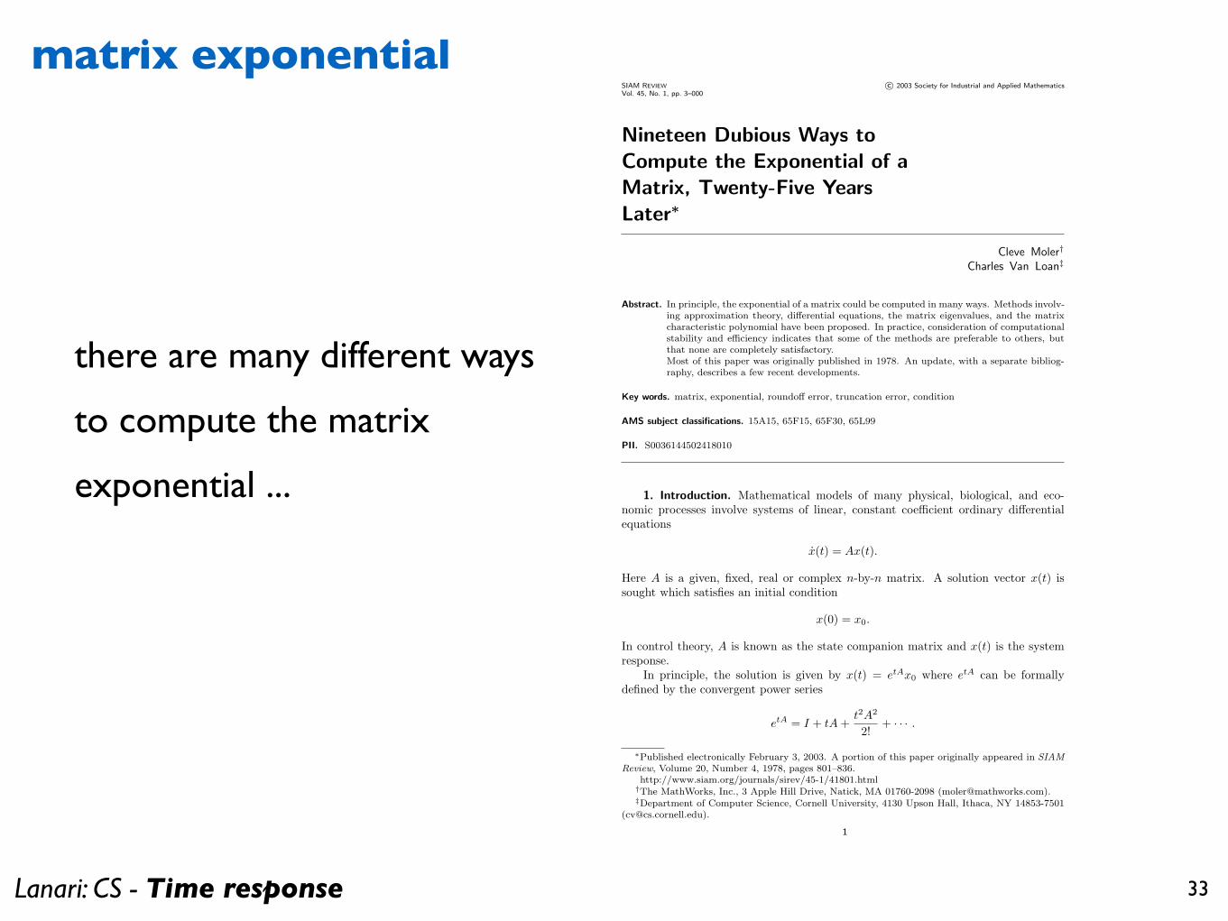
Lanari: CS - Time response 33
matrix exponentialSIAM REVIEW c∞ 2003 Society for Industrial and Applied MathematicsVol. 45, No. 1, pp. 3–000
Nineteen Dubious Ways to
Compute the Exponential of a
Matrix, Twenty-Five Years
Later§
Cleve Moler†
Charles Van Loan‡
Abstract. In principle, the exponential of a matrix could be computed in many ways. Methods involv-ing approximation theory, differential equations, the matrix eigenvalues, and the matrixcharacteristic polynomial have been proposed. In practice, consideration of computationalstability and efficiency indicates that some of the methods are preferable to others, butthat none are completely satisfactory.Most of this paper was originally published in 1978. An update, with a separate bibliog-raphy, describes a few recent developments.
Key words. matrix, exponential, roundoff error, truncation error, condition
AMS subject classifications. 15A15, 65F15, 65F30, 65L99
PII. S0036144502418010
1. Introduction. Mathematical models of many physical, biological, and eco-nomic processes involve systems of linear, constant coefficient ordinary differentialequations
x(t) = Ax(t).
Here A is a given, fixed, real or complex n-by-n matrix. A solution vector x(t) issought which satisfies an initial condition
x(0) = x0.
In control theory, A is known as the state companion matrix and x(t) is the systemresponse.
In principle, the solution is given by x(t) = etAx0 where etA can be formallydefined by the convergent power series
etA = I + tA +t2A2
2!+ · · · .
§Published electronically February 3, 2003. A portion of this paper originally appeared in SIAMReview, Volume 20, Number 4, 1978, pages 801–836.
http://www.siam.org/journals/sirev/45-1/41801.html†The MathWorks, Inc., 3 Apple Hill Drive, Natick, MA 01760-2098 ([email protected]).‡Department of Computer Science, Cornell University, 4130 Upson Hall, Ithaca, NY 14853-7501
1
there are many different ways
to compute the matrix
exponential ...
Lanari: CS - Time response 34
matrix exponential
z = eAz + eBu
y = eCz + eDux = Ax+Bu
y = Cx+Du
eeAtwith
“easier” to compute
eeAt = eTAT�1t = TeAtT�1eAt = T�1e
eAtT
“easier” to compute
9T :z = Txdet(T ) 6= 0
if
then
(proof)
we will use changes of coordinates (state) z = T x
Hypothesis
Lanari: CS - Time response 35
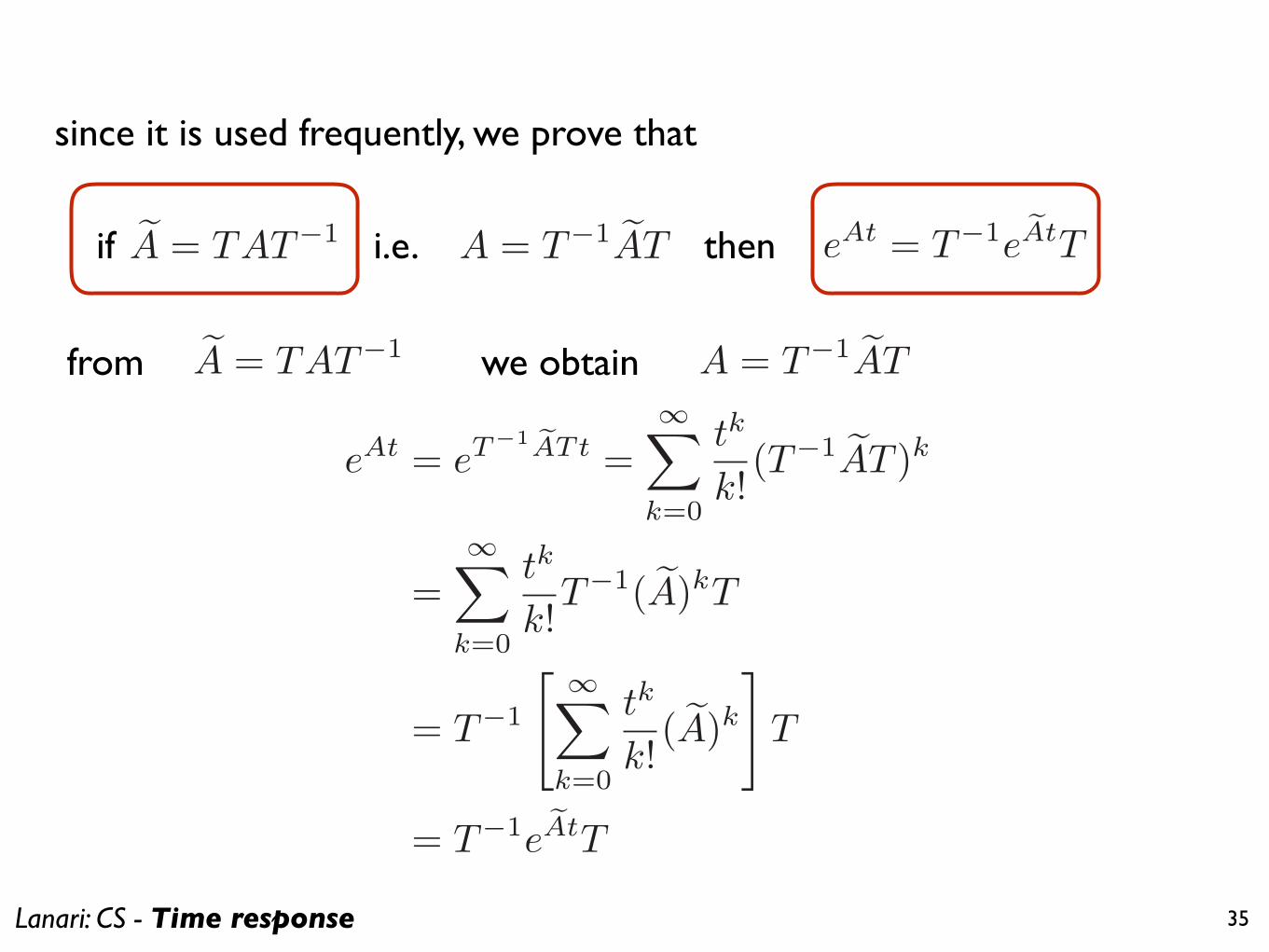
since it is used frequently, we prove that
A = T�1 eAT eAt = T�1eeAtT
eA = TAT�1
if then
from we obtain A = T�1 eAT
eAt = eT�1 eATt =
1X
k=0
tk
k!(T�1 eAT )k
=1X
k=0
tk
k!T�1( eA)kT
= T�1
" 1X
k=0
tk
k!( eA)k
#T
= T�1eeAtT
eA = TAT�1 i.e.
Lanari: CS - Time response 36
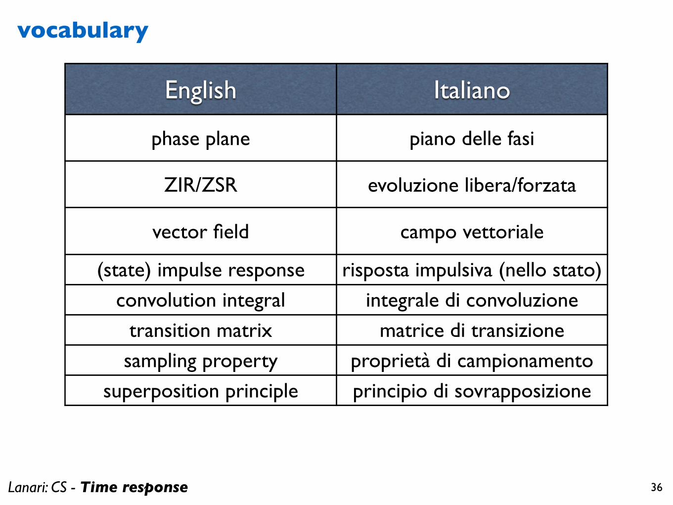
vocabulary
English Italiano
phase plane piano delle fasi
ZIR/ZSR evoluzione libera/forzata
vector field campo vettoriale
(state) impulse response risposta impulsiva (nello stato)convolution integral integrale di convoluzione
transition matrix matrice di transizionesampling property proprietà di campionamento
superposition principle principio di sovrapposizione


![lec03 feature.ppt [相容模式]](https://img.pdfslide.net/doc/110x75/6241df4175df7937e76cfeb3/lec03-.jpg)