© 2020 Sayed Hadi Hashemi

TIMED EXECUTIONIN DISTRIBUTED MACHINE LEARNING

BY

SAYED HADI HASHEMI

DISSERTATION

Submitted in partial fulfillment of the requirementsfor the degree of Doctor of Philosophy in Computer Science

in the Graduate College of theUniversity of Illinois at Urbana-Champaign, 2020

Urbana, Illinois

Doctoral Committee:

Professor Roy H. Campbell, ChairProfessor William D. GroppProfessor Philip B. GodfreyProfessor Volodymyr V. KindratenkoDr. Gregory F. Diamos

Abstract

Deep learning powers many transformative core technologies including Autonomous Driv-

ing, Natural Language Translation, and Automatic Medical Diagnosis. Its exceptional ability

to extract intricate structures from high-dimensional data takes the credit for major advances

in machine learning.

Essential ingredients that make Deep Learning possible include: the availability of a mas-

sive curated data, a well-designed model, and readily available high-performance computa-

tion. The computation used in training deep neural networks has doubled every 3.4 months

since 2012, five times faster than Moore’s law. Fulfilling this massive computational demand

that has long outgrown the capability of a single high-end node is vital to keep extending

the flow of innovations. For example, in 2018, the AlphaGoZero model trained with 1.89

ExaFlops/s times a day. The state-of-the-art GPU at the time, NVidia V-100, could only de-

liver 125 TeraFlops. In a meanwhile, Summit, the fastest supercomputer in the world, could

sustain 1 ExaFlops/s using 27,360 NVidia V-100 GPUs through distributed computation.

This dissertation studies the challenges of scaling out an ML job to keep up with the com-

putational demand, specifically the problems stemmed from the complex interplay of various

resources in the distributed ML. In the first stage of this research, we developed methods

and systems to properly observe a distributed ML environment by tracing a distributed

execution, visualizing the results, and expanding the observability to the production infras-

tructure. Later we developed three systems to address scalability challenges using these

methods and systems based on a precise execution timing of the spectrum of resources:

Network: TicTac reduces internal computation delays by enforcing a near-optimal order

on network transfers, which results in up to 37.7% throughput increases.

Computation: Caramel increases the network utilization and decreases network conges-

tion by modifying the order of computation and choosing the most fitted collective primitive

for the workload. This result in cutting the training time up by a factor of up to 3.8. While

computation and network scheduling suggest an order of execution, TimedRPC addresses the

issue of correctly enforcing this order by implementing a priority-based scheduling through

pre-emption where an on-going transfer can be paused when a transfer with higher priority

is requested.

ii

I/O: Diot maximizes the I/O throughput by tuning knobs such as number of concurrent

I/O requests and read size on I/O pipeline. Additionally it detects the I/O delivery unfairness

which may causes a struggling worker due to slow I/O through.

Thesis Statement

Heuristic timing of distributed machine learning execution leads to utilization optimiza-

tions for computation, network, and storage, which in turn improves the overall throughput.

In general, any multi-resource optimization involving parallelism is at least NP-Hard.

iii

To Shekoofeh, Reza, Akhtar, Amir, Azadeh, and Payam.

iv

Acknowledgments

Firstly, I would like to express my sincere gratitude to my advisor Professor Roy H Campbell, for

the continuous support of my research, for his patience, upbeat energy, motivation, and immense

knowledge. He was not only an advisor who helped to shape this study, but more importantly,

he was a mentor who forms me into a curious, confident, and independent researcher. It has been

a privilege for me to work with him and I could not have imagined having a better advisor and

mentor for my Ph.D. study.

Besides my advisor, I would like to thank the rest of my doctoral committee: Professor William

Gropp, Professor P. Brighten Godfrey, Professor Volodymyr Kindratenko, and Dr. Gregory Diamos,

for their invaluable feedback, insightful comments, and encouragement.

My sincere thanks also go to Dr. Bryan Catanzaro, Dr. Gregory Diamos, Dr. Paul Barham,

Professor Volodymyr Kindratenko, and the fantastic people at Baidu’s Silicon Valley Artificial

Intelligence Lab, Google Brain, and National Center for Supercomputing Applications who provided

me an opportunity to join their team. Without their precious support, it would not be possible to

conduct this research.

I thank my fellow collaborators throughout my journey. Mainly, I would like to thank Dr.

Sangeetha Abdu Jyothi for the inspirational discussions, and the sleepless nights, we were working

together before deadlines. I was fortunate to be part of ”Systems Research Group,” and many

thanks to its members, Dr. Faraz Faghri, Dr. Shadi A. Noghabi, Dr. Mohammad Babaeizadeh,

Dr. Read Sprabery, Dr. Chris Cai, Dr. Imani Palmer, Dr. Reza Farivar, Konstantin Evchenko,

and John Bellessa. I would also like to express my sincere gratitude to my many friends in Urbana-

Champaign for all the fun we have had in the last five years. Many thanks to the staff of the

Computer Science department, including but not limited to: Kathy Runck, Laura Thurlwell, Alice

Needham, Kara MacGregor, Mary Beth Kelley, Viveka Perera Kudaligama, and Maggie Metzger

Chappell for their continuous help and support during my studies.

Last but not least, I would like to thank my wife, my parents, my brothers and sister for the

unconditional love, and supporting me spiritually throughout this journey and my life in general.

v

TABLE OF CONTENTS

CHAPTER 1 INTRODUCTION . . . . . . . . . . . . . . . . . . . . . . . . . . . . 11.1 Contributions . . . . . . . . . . . . . . . . . . . . . . . . . . . . . . . . . . . 11.2 Modern Distributed Machine Learning Systems . . . . . . . . . . . . . . . . 31.3 Related Works . . . . . . . . . . . . . . . . . . . . . . . . . . . . . . . . . . . 4

CHAPTER 2 BACKGROUND . . . . . . . . . . . . . . . . . . . . . . . . . . . . . 62.1 Machine Learning . . . . . . . . . . . . . . . . . . . . . . . . . . . . . . . . . 62.2 Training Computation Model . . . . . . . . . . . . . . . . . . . . . . . . . . 82.3 Distributed Training Computation Model . . . . . . . . . . . . . . . . . . . . 102.4 Data Aggregation in Data-Parallel Distribution . . . . . . . . . . . . . . . . 11

CHAPTER 3 DISTRIBUTION CHALLENGES . . . . . . . . . . . . . . . . . . . . 133.1 Scaling Out Challenges . . . . . . . . . . . . . . . . . . . . . . . . . . . . . . 133.2 I/O Challenges . . . . . . . . . . . . . . . . . . . . . . . . . . . . . . . . . . 193.3 Methodological Challenges . . . . . . . . . . . . . . . . . . . . . . . . . . . . 22

CHAPTER 4 PERFORMANCE OBSERVABILITY IN DISTRIBUTED MACHINELEARNING . . . . . . . . . . . . . . . . . . . . . . . . . . . . . . . . . . . . . . . 244.1 Distributed Tracing . . . . . . . . . . . . . . . . . . . . . . . . . . . . . . . . 244.2 Visualization . . . . . . . . . . . . . . . . . . . . . . . . . . . . . . . . . . . 264.3 Tracing in Production . . . . . . . . . . . . . . . . . . . . . . . . . . . . . . 30

CHAPTER 5 I/O IN DISTRIBUTED MACHINE LEARNING . . . . . . . . . . . 355.1 Background . . . . . . . . . . . . . . . . . . . . . . . . . . . . . . . . . . . . 365.2 Diot . . . . . . . . . . . . . . . . . . . . . . . . . . . . . . . . . . . . . . . . 385.3 Experimental Study . . . . . . . . . . . . . . . . . . . . . . . . . . . . . . . . 405.4 Conclusion . . . . . . . . . . . . . . . . . . . . . . . . . . . . . . . . . . . . . 44

CHAPTER 6 COMMUNICATION SCHEDULING OF CAUSAL DEPENDENCIES 456.1 Introduction . . . . . . . . . . . . . . . . . . . . . . . . . . . . . . . . . . . . 456.2 Background and Motivation . . . . . . . . . . . . . . . . . . . . . . . . . . . 476.3 Quantifying Performance . . . . . . . . . . . . . . . . . . . . . . . . . . . . . 496.4 Scheduling Algorithms . . . . . . . . . . . . . . . . . . . . . . . . . . . . . . 526.5 System Design . . . . . . . . . . . . . . . . . . . . . . . . . . . . . . . . . . . 566.6 Results . . . . . . . . . . . . . . . . . . . . . . . . . . . . . . . . . . . . . . . 596.7 TIC vs. TAC . . . . . . . . . . . . . . . . . . . . . . . . . . . . . . . . . . . 616.8 Conclusion . . . . . . . . . . . . . . . . . . . . . . . . . . . . . . . . . . . . . 66

vi

CHAPTER 7 ACHIEVING NETWORK EFFICIENCY THROUGH COMPU-TATION SCHEDULING . . . . . . . . . . . . . . . . . . . . . . . . . . . . . . . . 687.1 Introduction . . . . . . . . . . . . . . . . . . . . . . . . . . . . . . . . . . . . 687.2 Background . . . . . . . . . . . . . . . . . . . . . . . . . . . . . . . . . . . . 707.3 Motivation . . . . . . . . . . . . . . . . . . . . . . . . . . . . . . . . . . . . . 717.4 Caramel Design . . . . . . . . . . . . . . . . . . . . . . . . . . . . . . . . . 757.5 Implementation . . . . . . . . . . . . . . . . . . . . . . . . . . . . . . . . . . 797.6 Experiments . . . . . . . . . . . . . . . . . . . . . . . . . . . . . . . . . . . . 807.7 Discussion . . . . . . . . . . . . . . . . . . . . . . . . . . . . . . . . . . . . . 857.8 Enforcing the Execution Timing Through Timed RPC . . . . . . . . . . . . 867.9 Related Work . . . . . . . . . . . . . . . . . . . . . . . . . . . . . . . . . . . 887.10 Conclusion . . . . . . . . . . . . . . . . . . . . . . . . . . . . . . . . . . . . . 90

CHAPTER 8 CONCLUSION . . . . . . . . . . . . . . . . . . . . . . . . . . . . . . 918.1 Limitations . . . . . . . . . . . . . . . . . . . . . . . . . . . . . . . . . . . . 918.2 Future Works . . . . . . . . . . . . . . . . . . . . . . . . . . . . . . . . . . . 92

REFERENCES . . . . . . . . . . . . . . . . . . . . . . . . . . . . . . . . . . . . . . . 94

vii

CHAPTER 1: INTRODUCTION

Artificial intelligence and in particular Deep Neural Networks (DNNs) form the crux of

the advanced solutions in a variety of fields such as computer vision, speech recognition,

autonomous driving, and natural language processing. The availability of rich data, readily

accessible distributed high-performance computing, and flexibility of development offered by

modern machine learning systems fuel AI growth in the past decade.

The computational cost of training sophisticated deep learning models has long outgrown

the capabilities of a single high-end machine, leading to distributed training being the norm

in a typical AI pipeline. Scaling from a single machine to multi-node training brings exciting

challenges on how to handle communication, which has a crucial impact on the performance

and scalability of distributed ML applications.

Adding networking to a machine learning job creates a complex interplay of heterogeneous

resources which demands precise timing of network transfers, computational operations, and

I/O requests to sustain a full resource utilization.

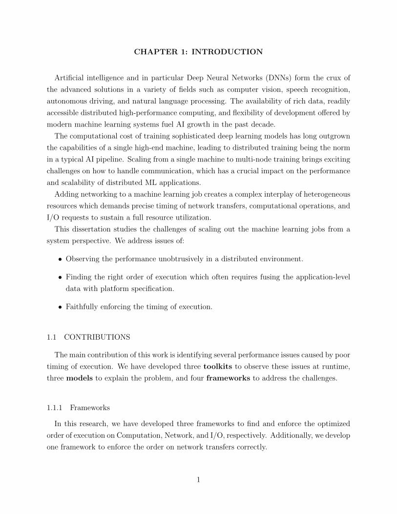
This dissertation studies the challenges of scaling out the machine learning jobs from a

system perspective. We address issues of:

• Observing the performance unobtrusively in a distributed environment.

• Finding the right order of execution which often requires fusing the application-level

data with platform specification.

• Faithfully enforcing the timing of execution.

1.1 CONTRIBUTIONS

The main contribution of this work is identifying several performance issues caused by poor

timing of execution. We have developed three toolkits to observe these issues at runtime,

three models to explain the problem, and four frameworks to address the challenges.

1.1.1 Frameworks

In this research, we have developed three frameworks to find and enforce the optimized

order of execution on Computation, Network, and I/O, respectively. Additionally, we develop

one framework to enforce the order on network transfers correctly.

1

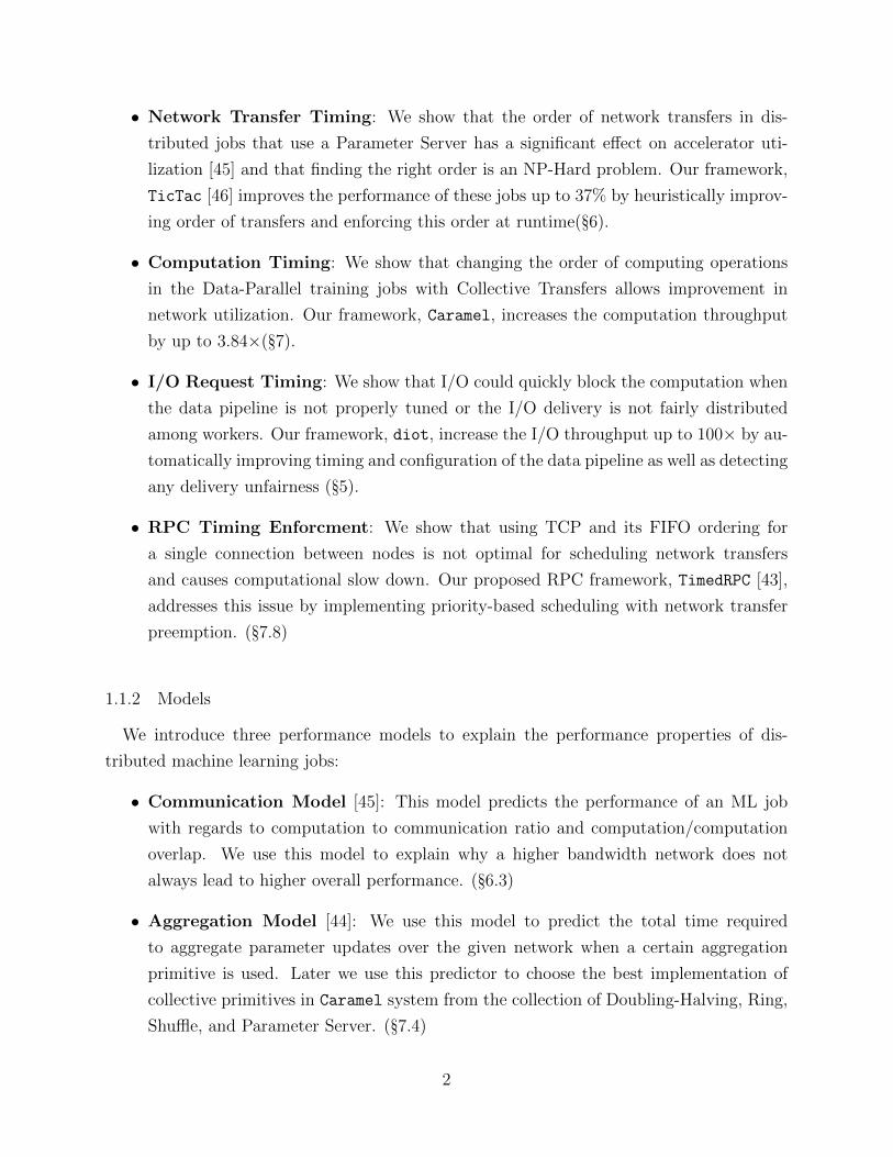
• Network Transfer Timing: We show that the order of network transfers in dis-

tributed jobs that use a Parameter Server has a significant effect on accelerator uti-

lization [45] and that finding the right order is an NP-Hard problem. Our framework,

TicTac [46] improves the performance of these jobs up to 37% by heuristically improv-

ing order of transfers and enforcing this order at runtime(§6).

• Computation Timing: We show that changing the order of computing operations

in the Data-Parallel training jobs with Collective Transfers allows improvement in

network utilization. Our framework, Caramel, increases the computation throughput

by up to 3.84×(§7).

• I/O Request Timing: We show that I/O could quickly block the computation when

the data pipeline is not properly tuned or the I/O delivery is not fairly distributed

among workers. Our framework, diot, increase the I/O throughput up to 100× by au-

tomatically improving timing and configuration of the data pipeline as well as detecting

any delivery unfairness (§5).

• RPC Timing Enforcment: We show that using TCP and its FIFO ordering for

a single connection between nodes is not optimal for scheduling network transfers

and causes computational slow down. Our proposed RPC framework, TimedRPC [43],

addresses this issue by implementing priority-based scheduling with network transfer

preemption. (§7.8)

1.1.2 Models

We introduce three performance models to explain the performance properties of dis-

tributed machine learning jobs:

• Communication Model [45]: This model predicts the performance of an ML job

with regards to computation to communication ratio and computation/computation

overlap. We use this model to explain why a higher bandwidth network does not

always lead to higher overall performance. (§6.3)

• Aggregation Model [44]: We use this model to predict the total time required

to aggregate parameter updates over the given network when a certain aggregation

primitive is used. Later we use this predictor to choose the best implementation of

collective primitives in Caramel system from the collection of Doubling-Halving, Ring,

Shuffle, and Parameter Server. (§7.4)

2

• Storage Model [47]: We use this model initially to explain the poor performance of

CNTK on BlueWaters where I/O was the bounding resource [47]. Later we use this

model to predict when the I/O becomes a bottleneck in an ML job. (§5)

1.1.3 Toolkits

We have developed a collection of performance analysis toolkits to bring runtime trans-

parency into the execution of distributed machine learning jobs:

• Distributed Tracing: We expand the execution tracing capability of the existing

system to support multi-machine jobs. This toolkit [42] coordinate the tracing among

all the workers, captures the network activities (encapsulated as RPC calls) on all

workers, and collect all the traces without interfering with the execution. (§4)

• Visualization: We develop a visualization toolkit [42] to facilitate the examination of

a large quantity of tracing data by providing fast navigation of events while retaining

the event details. (§4.2)

• Tracing in the Production: We extend the distributed tracing to production infras-

tructures. tensorflow-tracer [48] allows system administrators to profile and trace

ML jobs without any code modifications and exchange tracing sessions to developers.

(§4.3)

1.2 MODERN DISTRIBUTED MACHINE LEARNING SYSTEMS

There has been many distributed ML system introduced in the past few years. Ten-

sorFlow [1], PyTorch [81], Microsoft Cognitive Toolkit [89], Keras [26], MXNet [21], and

Chainer [104] to name a few. While there are many differences between these systems, they

can be characterized by three main traits:

1. Iterative: Modern systems focus on training large ML models on a big dataset which

requires more sophisticated optimizer such as the family of “Stochastic Gradient De-

scent” algorithms [15, 85, 62, 86, 16]. These optimizers are iterative; The training

process is a series of iterations which read a batch of data and update a set of persis-

tent parameters. All the modern systems are designed around this iterative workload.

2. Compute Intensive: The massive success of Deep Learning which requires substan-

tial computation time on the training makes specialized accelerators, such as the GPU

3

and TPU [59], a standard part of ML infrastructure and natively supported by ML sys-

tems. To contain the steep learning curve of SIMD programming for these accelerators,

the ML workload is represented as a DAG of predefined operations.

3. Rapid Experimentation: The fast pace of change in AI requires a shorter cycle of

prototyping an idea to getting results. To this end, the current incarnation of ML

introduces dataFlow DAGs to hide the steep learning curve of SIMD programming for

specialized accelerators and gradient calculations in SGD.

1.3 RELATED WORKS

This section presents an overview of evolution of distributed machine learning from the

early cloud computing era until present days.

MapReduce The success of MapReduce [32] computational models in cloud computing

inspires early distributed machine learning systems. Examples of these systems are Apache

Mahout [53] (2009) built on top of Hadoop ecosystem [107] and MLlib [72] (2013) built on

top of Spark Ecosystem [115]. These systems are a collection of computationally-light ML

algorithms implemented as Map/Reduce jobs. Using MapReduce in these systems allowed

the ML algorithms to be applied to the massive data stored in the cloud.

Parameter Server The next wave of Distributed ML systems makes use of the Parameter

Server (PS) architecture to support more customizable and complicated ML models and

iterative training algorithms such as Stochastic Gradient Descent [85, 62, 86, 16]. Examples

are DistBelief [31] in 2012 and Project Adam [24] in 2014 which are designed specifically for

neural networks and Parameter Server[68] in 2014 designed for some simpler models. In this

architecture, the ML parameters are stored and managed in parameter servers (PS) modeled

after Key-Value systems with weak consistency. At the beginning of an iteration, a worker

reads the recent version of parameters from PS, then sends the updates back to the PS at

the end.

GPU and Deep Learning Breakthrough In 2012, AlexNet [64] substantially reduced

the error rate in the ”ImageNet Large Scale Visual Recognition Competition” using a neural

network trained on the GPU. The success of this work made a paradigm shift to ML research:

Use of higher capacity neural network models (dubbed as Deep Learning [67]) which required

higher computation time that could be cheaply attained using the GPUs of the time. The

4

steep learning curve of developing GPU application led to a new DAG-based programming

model introduced in Caffe [58] and MxNet [21]. In this model, the workload is represented

as a DAG where nodes are operations and edges are data flow or control dependencies. The

ML framework is shipped with predefined operations with GPU implementations. The user

then define the data flow or dependencies without requiring any GPU programming. Using

a DAG-based model has been widely adapted in recent iterative machine learning systems.

TensorFlow [1] in 2015 extends this representation by assigning nodes to each device as

well as adding network transfers as nodes to the DAG. This unified representation permits

compiler optimizations and simplifies deployment [17].

Collective Transfers Moving beyond PS architecture, DeepSpeech2 in 2015 [7] and CNTK

in 2016 [89] proposed a new distribution architecture tailored toward high-performance net-

works such as Infiniband and Omnipath. In these systems, unlike PS architecture, there are

no centralized servers. Each worker stores a copy of parameters and update to parameters

as an aggregate through a collective transfer such as MPI allreduce call in MPI[40]. This

is accelerated by hardware and unlike PS, it does not induce network congestion.

Later in 2017, these collective transfers are added to the collection of predefined operations

in data flow DAG as operations by Baidu Allreduce [11] and Horovod [90].

In 2017, Facebook [37] reduced the training time of ResNet-50 from 29 hours to less than

an hour while maintaining the same level of accuracy by combining the collective transfer

architecture with enormous mini-batch sizes increased from 256 to 8192. This work has been

the basis of a large number of followup works pushing the computation boundaries further

[57, 4, 112, 113] including Exascale Deep Learning for Climate Analytics [65] on Summit

SuperComputer which broke the ExaFlop barrier of an Application for the first time.

Beyond DAG The DAG has been the dominant representation of ML workloads, search

for alternatives continue. PyTorch [81] and other works [3, 77]introduce imperative DAG

programming style. In this style, an operation is executed as soon as it is added to the DAG.

This, in turn, improves the interactive experience of a developer by allowing just in time

debugging and more natural flow of execution.

Yu et al. [114] propose a new graph-based representation which adds conditional branching

and loops to dataflow DAGs while maintaining the support for automatic differentiation.

The DAG programming style with coarse hyper-optimized predefined operations is blamed

for hindering ML research progress [12] by making it harder to experiment with new oper-

ation types. Addressing this problem inspires high-performance general-purpose numerical

programming models coupled with device agnostics compilers [54, 22, 103].

5

CHAPTER 2: BACKGROUND

“All models are wrong; some models are useful.”

George E. P. Box

The goal of this chapter is to introduce the computational model of distributed ML jobs.

To this end, the chapter starts with the definition of ML and the optimization problem it

needs to solve. Then, the stochastic gradient descent (SGD) is introduced as a promising

solution. Later we discuss how distributed SGD is implemented in ML systems.

2.1 MACHINE LEARNING

Machine learning as a subset of Artificial Intelligence is the scientific study of making a

system learn a task without being explicitly programmed to do so. Mitchell [76] defines

learning as:

“A computer program is said to learn from experience E with respect to some

class of tasks T and performance measure P , if its performance at tasks in T , as

measured by P , improves with experience E.”

Tasks refer to how a machine should process an example [36]. For instance, a Classifi-

cation task assigns a class, from a limited list, to a given example. An example is usually

defined as a set of features.

Performance Measure quantitatively evaluates the performance of a machine learning

algorithm. For example, in a classification task, Accuracy is a performance measure that

shows the proportion of examples for which the model assigned the right class.

Experiments are a collection of examples, or methods used in obtaining the data or

examples that an algorithm has access to during the learning process [36]. For example, in a

Supervised environment, an algorithm has access to a labeled dataset, which is a collection of

examples each associated with a class. A Experiment set in supervised learning is commonly

called a dataset.

6

2.1.1 Example: Supervised Classification

To better understand the computation model of an ML job, this section describes a simple

“Classification” learning task with a “Supervised” experiment. In this experiment, the

dataset is:

X ∈ Rn,Y ∈ C = {c1, c2, . . . , cm},X → Y (2.1)

Where X is the set of examples with n features and Y is the set of classes. Each example

is associated with a class.

The classification task is defined as function which assigns a class to a given example:

f(W ;x) : Rn → C (2.2)

f is the machine learning model, such as Neural Networks or Linear Class, and W is a set

of parameters the model takes in addition to an example, x.

The goal of learning is to optimize performance measure. For example, Using a loss

function as the measure, the optimization problem is:

minf ,W

loss(f(W ;X),Y ) (2.3)

Training a given model f , is the process of optimizing W :

minW

loss(f(W ;X),Y ) (2.4)

2.1.2 Stochastic Gradient Descent

As the size parameters and dataset grow, it becomes harder to solve the optimization

problem in 2.4. Stochastic Gradient Descent and its variations [85, 62, 86, 16, 67] are the

de facto methods in these cases.

The main idea in this iterative optimizer is to follow the opposite direction of the perfor-

mance measure gradient. In each iteration, randomly selected examples, Xbs and Ybs, are

used to calculate the gradient. Then a multiplier of the gradient is subtracted from the

parameters:

W ← W − η∇loss(f(W ;Xbs),Ybs) (2.5)

Where η is the learning rate, and bs is the mini-batch size. There are three tasks involved

in machine learning:

7

Parameters

Read Update

Input Data

(a) Architecture

Load Forward Pass

Read

Backward Propagation UpdateProcessor/Accelarator

(b) Timeline

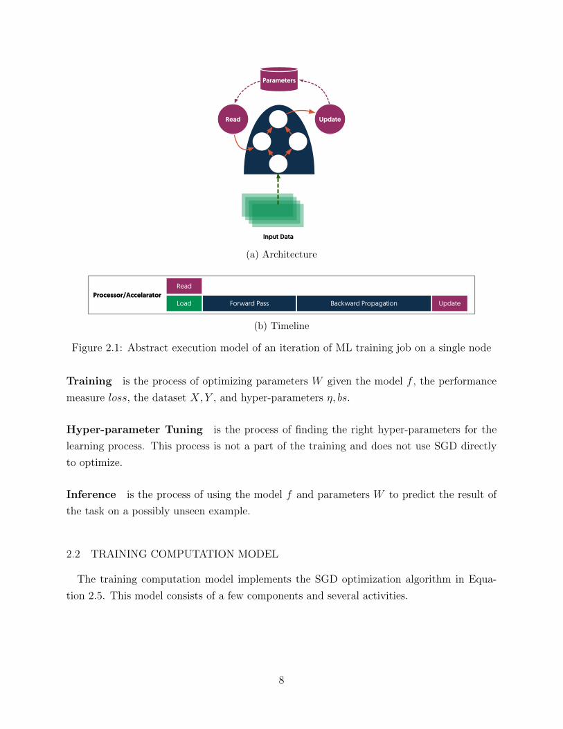
Figure 2.1: Abstract execution model of an iteration of ML training job on a single node

Training is the process of optimizing parameters W given the model f , the performance

measure loss, the dataset X,Y , and hyper-parameters η, bs.

Hyper-parameter Tuning is the process of finding the right hyper-parameters for the

learning process. This process is not a part of the training and does not use SGD directly

to optimize.

Inference is the process of using the model f and parameters W to predict the result of

the task on a possibly unseen example.

2.2 TRAINING COMPUTATION MODEL

The training computation model implements the SGD optimization algorithm in Equa-

tion 2.5. This model consists of a few components and several activities.

8

2.2.1 Components

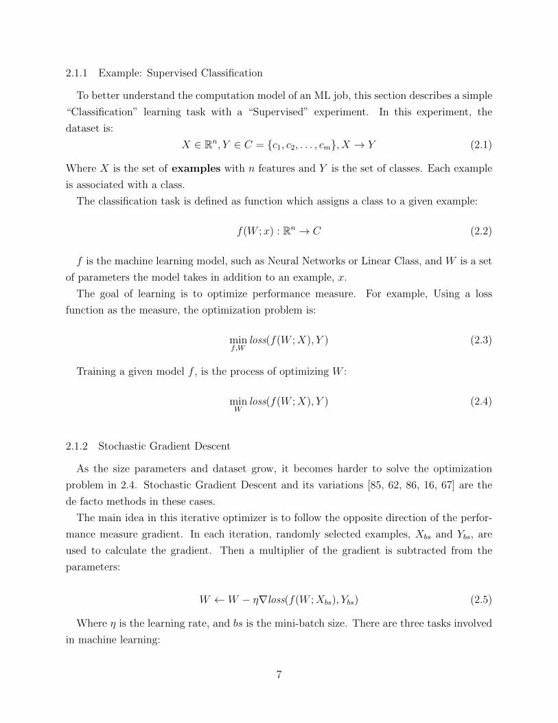
The training computation model includes the following components (Figure 2.1a):

Stateless DAG: The logic of machine learning model, including calculating the loss func-

tion and gradients is represented by a stateless DAG where nodes are predefined operations

and edges are data or control dependencies.

Stateful Parameters: The parameters are stored in a persistent object-store shared

among ops in the DAG. Special nodes of the DAG can read and update parameters in

this object-store.

Input Data: Dataset is stored in a secondary storage. Parallel to the training, the data

is read from the storage and preprocessed. The DAG then reads this already loaded and

transformed data in each iteration.

2.2.2 Activities

In each iteration, the DAG reads a batch of examples from the dataset and parameters

from the persistent object-store. Then loss function and gradients are calculated, and the

gradients are applied to the parameters.

Figure 2.1b shows the timeline of the execution. There are five distinct activities in this

timeline. Each activities consist of multiple ops which are part of the DAG:

Loading Input Data: The first step of the iteration is to load the input data from

memory to the accelerator memory. The data is loaded and preprocessed from a storage

asynchronously with the computation (§5.1).

Reading Parameters: This starts in parallel to loading the input data; Each parameter

is read individually from the persistent object-store.

Forward Pass: This calculates the loss function using the input data and parameters.

The execution of forward-pass, like the rest of the DAG, follows topological order. An op

is ready to execute if all its dependencies are available. Therefore, some ops in forward

pass may start before all the parameters are loaded. Forward pass also temporary keeps the

intermediate data to be used in backward propagations.

9

Backward Propagation: This calculates the gradients of each parameter following the

chain rule. This component runs after the forward pass finishes and uses the loss function

value and the intermediate data. Gradients of parameters are calculated roughly in the

reverse order the parameters are used in the forward pass.

Updating Parameters: This implements the rule of SGD or other optimizers to update

the parameters using the gradients. In this component, the updated value is stored in the

persistent object-store. Whenever a gradient is calculated, its corresponding parameter may

be updated without waiting for the rest of the Backward Propagation finishes.

An iteration finishes when all the nodes in the DAG are executed.

2.3 DISTRIBUTED TRAINING COMPUTATION MODEL

Distributing a ML jobs introduces network ops and device associations, where each node

in the dataFlow DAG is associated with a device. There are three major ways to divide

the computation load on multiple devices: Examples, DataFlow DAG, and Operations, or a

combination of these three.

Examples In this approach, the mini-batch input is divided among workers. Each worker

has a replica of the dataflow and aggregates the parameter changes with other workers.

This approach is known as Data-Parallel or Model-Replica. Scaling a model using a Data-

Parallel approach is easier compared to other distribution approaches and does not require

any placement or human intervention. For example, Data-Parallel DeepLabv3+ [20] has

been scaled out to 27360 GPUs while sustaining parallel efficiency of 90.7% [65].

DataFlow DAG In this approach, the dataflow DAG is partitioned on multiple devices.

Each worker hosts a part of the DAG. If two ends of an edge are located on different

devices, the data is transferred using network or other communication channels (e.g. PCI

Express). This approach is known as Model-Parallel. Model-Parallel is shown to have a

better performance than Data-Parallel [74, 75]. However, partitioning and placement of

the DAG is a non-trivial task that has to be done either manually or by approximation

algorithms which in practice can not handle more than a few workers (4 GPUs in [74] and

8 GPUs in [75]).

Operations In this approach, one operation is divided over multiple devices. This ap-

proach is mainly used when an operation is disproportionally compute-expensive or exceed

10

Parameter Server

Worker

Read Update

Worker

Read Update

Worker

Read Update

Parameters

(a) Architecture

Load Forward Pass

Read P1

Backward Propagation

Send !P2Read P2 Send !P1Network

Processor/Accelarator

(b) Timeline

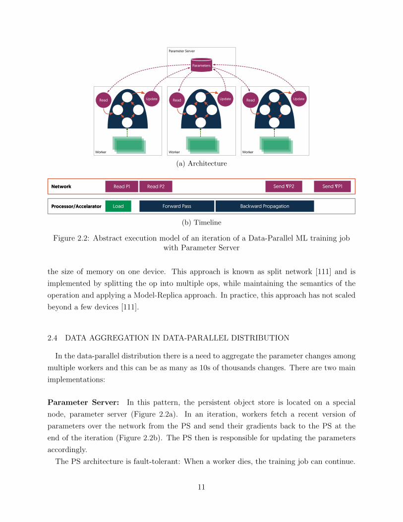
Figure 2.2: Abstract execution model of an iteration of a Data-Parallel ML training jobwith Parameter Server

the size of memory on one device. This approach is known as split network [111] and is

implemented by splitting the op into multiple ops, while maintaining the semantics of the

operation and applying a Model-Replica approach. In practice, this approach has not scaled

beyond a few devices [111].

2.4 DATA AGGREGATION IN DATA-PARALLEL DISTRIBUTION

In the data-parallel distribution there is a need to aggregate the parameter changes among

multiple workers and this can be as many as 10s of thousands changes. There are two main

implementations:

Parameter Server: In this pattern, the persistent object store is located on a special

node, parameter server (Figure 2.2a). In an iteration, workers fetch a recent version of

parameters over the network from the PS and send their gradients back to the PS at the

end of the iteration (Figure 2.2b). The PS then is responsible for updating the parameters

accordingly.

The PS architecture is fault-tolerant: When a worker dies, the training job can continue.

11

Worker

Read

Parameter

Worker

Read

UpdateParameter

Worker

Read

UpdateParameterUpdate

(a) Architecture

Processor/AccelaratorLoad Forward Pass

Read

Backward Propagation

Aggregate !P1

Network

Update P2

Update P2

Aggregate !P2

(b) Timeline

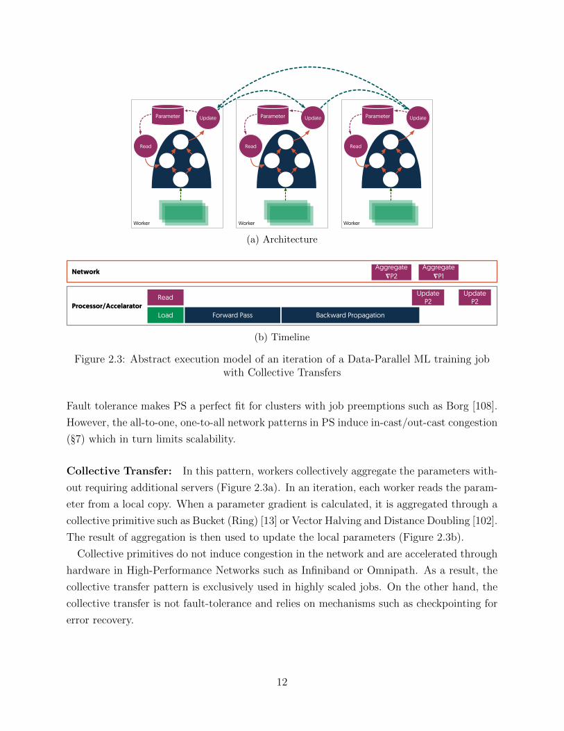
Figure 2.3: Abstract execution model of an iteration of a Data-Parallel ML training jobwith Collective Transfers

Fault tolerance makes PS a perfect fit for clusters with job preemptions such as Borg [108].

However, the all-to-one, one-to-all network patterns in PS induce in-cast/out-cast congestion

(§7) which in turn limits scalability.

Collective Transfer: In this pattern, workers collectively aggregate the parameters with-

out requiring additional servers (Figure 2.3a). In an iteration, each worker reads the param-

eter from a local copy. When a parameter gradient is calculated, it is aggregated through a

collective primitive such as Bucket (Ring) [13] or Vector Halving and Distance Doubling [102].

The result of aggregation is then used to update the local parameters (Figure 2.3b).

Collective primitives do not induce congestion in the network and are accelerated through

hardware in High-Performance Networks such as Infiniband or Omnipath. As a result, the

collective transfer pattern is exclusively used in highly scaled jobs. On the other hand, the

collective transfer is not fault-tolerance and relies on mechanisms such as checkpointing for

error recovery.

12

CHAPTER 3: DISTRIBUTION CHALLENGES

“You can have a second computer once you’ve shown youknow how to use the first one.”

Paul Barham

Distribution allows more computational resources to be made available for a job. However,

fully utilizing the resource increase is quite challenging. This chapter is a summary of such

challenges, many have been reported first by this work. We classify these issues into three

categories:

• Scaling Out Challenges: These appear when the network is added to a ML job

including Slow Network, Poor Timing, and Network Underutilization.

• I/O Challenges: These are about reading the data from the storage. Slow Storage,

Storage Underutilization, and Delivery Unfairness.

• Methodological Challenges: These limit the available options to address a per-

formance issue. These options are bounded by how intrusive the solution is to the

underlying ML logic.

Furthermore, this chapter describes how the rest of this dissertation addresses these issues.

3.1 SCALING OUT CHALLENGES

Scaling out an ML job does not always improve the overall performance despite the added

capacity. In this section, we discuss some of the reasons and how to mitigate them.

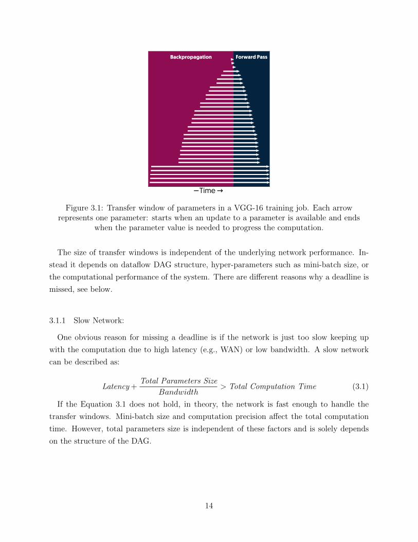
The transfer window of a parameter is a period on DAG from when the parameter gradient

is calculated in back-propagation to when the updated value is read which could be in the

next iteration. If the gradient aggregation among multiple workers finishes after the end of

the transfer window, the computation on workers will be stalled waiting for the aggregation

to finish. Therefore, for the maximum computational utilization the network transfers should

finish within the parameter windows. Figure 3.1 shows the transfer window of VGG-19 [95]

running on a slightly modified TensorFlow (§7). Each arrow represents the transfer window

of one parameter. As long as all the parameters are updated in their window, the ML job

can be perfectly scaled as far as the network concerns. Updating the parameters faster does

not speed up the training; however, missing the window slows down the training since the

accelerator has to stay idle waiting for the parameter.

13

Time

Backpropagation Forward Pass

Figure 3.1: Transfer window of parameters in a VGG-16 training job. Each arrowrepresents one parameter: starts when an update to a parameter is available and ends

when the parameter value is needed to progress the computation.

The size of transfer windows is independent of the underlying network performance. In-

stead it depends on dataflow DAG structure, hyper-parameters such as mini-batch size, or

the computational performance of the system. There are different reasons why a deadline is

missed, see below.

3.1.1 Slow Network:

One obvious reason for missing a deadline is if the network is just too slow keeping up

with the computation due to high latency (e.g., WAN) or low bandwidth. A slow network

can be described as:

Latency +Total Parameters Size

Bandwidth> Total Computation Time (3.1)

If the Equation 3.1 does not hold, in theory, the network is fast enough to handle the

transfer windows. Mini-batch size and computation precision affect the total computation

time. However, total parameters size is independent of these factors and is solely depends

on the structure of the DAG.

14

Fig

ure

3.2:

The

exec

uti

onti

mel

ine

ofa

trai

nin

git

erat

ion.

The

hor

izon

tal

axis

repre

sents

tim

e;ea

chb

oxre

pre

sents

anop

exec

uti

on.

The

arbit

rary

tran

sfer

tim

ing

indef

ault

Ten

sorF

low

cause

spro

cess

ing

tost

ale

wai

ting

for

net

wor

ktr

ansf

ers.

15

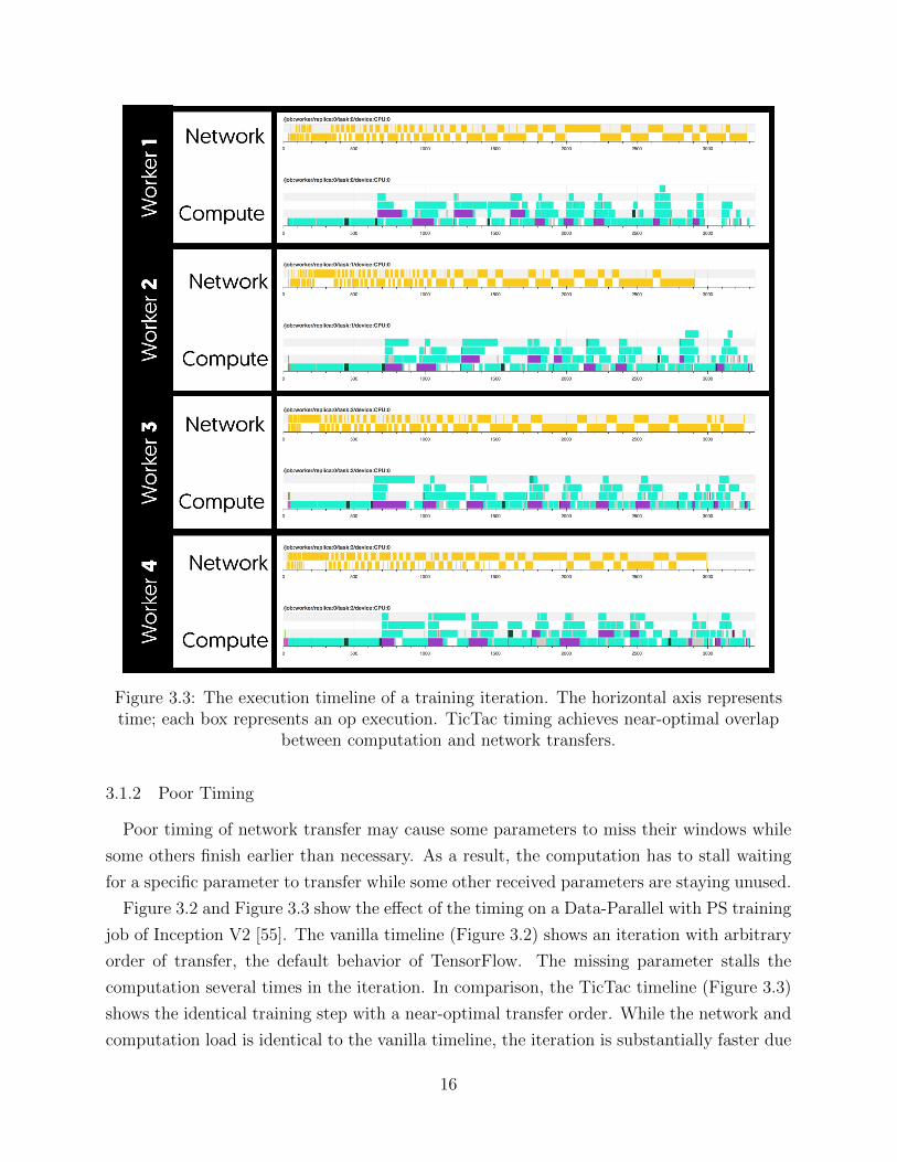
Figure 3.3: The execution timeline of a training iteration. The horizontal axis representstime; each box represents an op execution. TicTac timing achieves near-optimal overlap

between computation and network transfers.

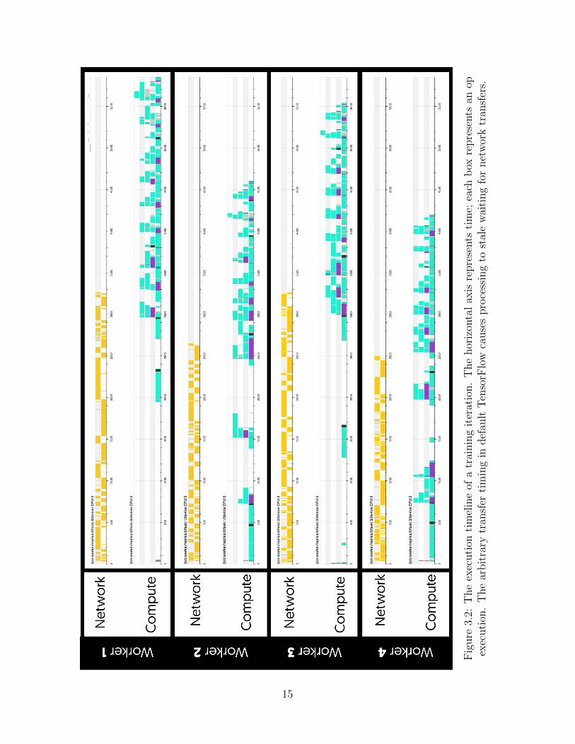
3.1.2 Poor Timing

Poor timing of network transfer may cause some parameters to miss their windows while

some others finish earlier than necessary. As a result, the computation has to stall waiting

for a specific parameter to transfer while some other received parameters are staying unused.

Figure 3.2 and Figure 3.3 show the effect of the timing on a Data-Parallel with PS training

job of Inception V2 [55]. The vanilla timeline (Figure 3.2) shows an iteration with arbitrary

order of transfer, the default behavior of TensorFlow. The missing parameter stalls the

computation several times in the iteration. In comparison, the TicTac timeline (Figure 3.3)

shows the identical training step with a near-optimal transfer order. While the network and

computation load is identical to the vanilla timeline, the iteration is substantially faster due

16

0.00 0.25 0.50 0.75 1.00 1.25 1.50 1.75 2.00Communication to Computation Ratio ( )

0.0

0.2

0.4

0.6

0.8

1.0O

verla

p C

oeffi

cien

t ()

Better Performance

35%

40%

45%

50%

55%

60%

65%70%

75%

80%

85%

90%

95%

99%

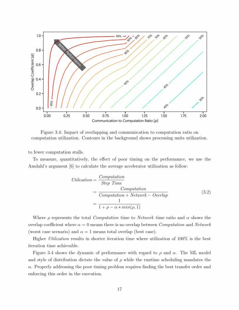
Figure 3.4: Impact of overlapping and communication to computation ratio oncomputation utilization. Contours in the background shows processing units utilization.

to fewer computation stalls.

To measure, quantitatively, the effect of poor timing on the performance, we use the

Amdahl’s argument [6] to calculate the average accelerator utilization as follow:

Utilization =Computation

Step Time

=Computation

Computation + Network−Overlap

=1

1 + ρ− α ∗min(ρ, 1)

(3.2)

Where ρ represents the total Computation time to Network time ratio and α shows the

overlap coefficient where α = 0 means there is no overlap between Computation and Network

(worst case scenario) and α = 1 means total overlap (best case).

Higher Utilization results in shorter iteration time where utilization of 100% is the best

iteration time achievable.

Figure 3.4 shows the dynamic of performance with regard to ρ and α. The ML model

and style of distribution dictate the value of ρ while the runtime scheduling mandates the

α. Properly addressing the poor timing problem requires finding the best transfer order and

enforcing this order in the execution.

17

Finding the Best Order The DAG representation of ML workloads creates a complex

resource interdependency which in turn, complicates the process of finding the best order.

Following the notion in [83], the scheduling problem of finding the best execution order in a

Data-Parallel job with identical nodes is formally defined as:

Pm|Mi, prec|Cmax (3.3)

In this formulation, Pm represents multiple parallel resources with identical performance. Mi

assigns the operations to specific resources, i.e., computation ops vs. communication. prec

describes the dependency relation of ops that is the DataFlow DAG. The Cmax represents

the goal of scheduling is to minimize the last node completion time.

This problem is still open [19] and simpler cases are proven to be NP-Hard. While there

exist approximations for relaxed versions of this problem, to the best of our knowledge, there

is no solution or approximation with guaranteed bounds for our original problem.

In §6, we present two approximations to this problem with empirically near-optimal results.

Enforcing the Best Order: Using TCP would imply an in-order delivery of the data,

which is irrespective of priorities based on best transfer order. To enforce a transfer order

beyond FIFO, a priority-based scheduling is needed where priorities are the order of execu-

tion. This scheduling scheme should additionally support pre-emption to pause a transfer if

a higher priority transfer is requested. Our application-aware RPC framework, Timed RPC,

implements the priority-based scheduling on top of the existing TCP based network stack.

It mimics the transfer pre-emption by splitting each transfer into smaller pieces. (§7.8).

3.1.3 Network Underutilization

The ML job may not be able to use the full network bandwidth for the whole duration of

the iteration. For example, if p is the average portion of full network bandwidth that a job

uses during an iteration, the transfer windows are missed if:

Latency +Total Parameters Size

Bandwidth× p> Total Computation Time (3.4)

As the network to computation ratio increases, which naturally happens in scaling out, the

effect of underutilized network becomes more severe.

There are two common root causes for the network underutilization:

18

0.0 0.2 0.4 0.6 0.8 1.0 1.2 1.4Communication to Computation Ratio ( )

0.0

0.2

0.4

0.6

0.8

1.0O

verla

p C

oeffi

cien

t ()

TensorFlow + MPI

TensorFlow + PS

35%

40%

45%

50%

55%

60%

65%70%

75%

80%

85%

90%

95%

99%

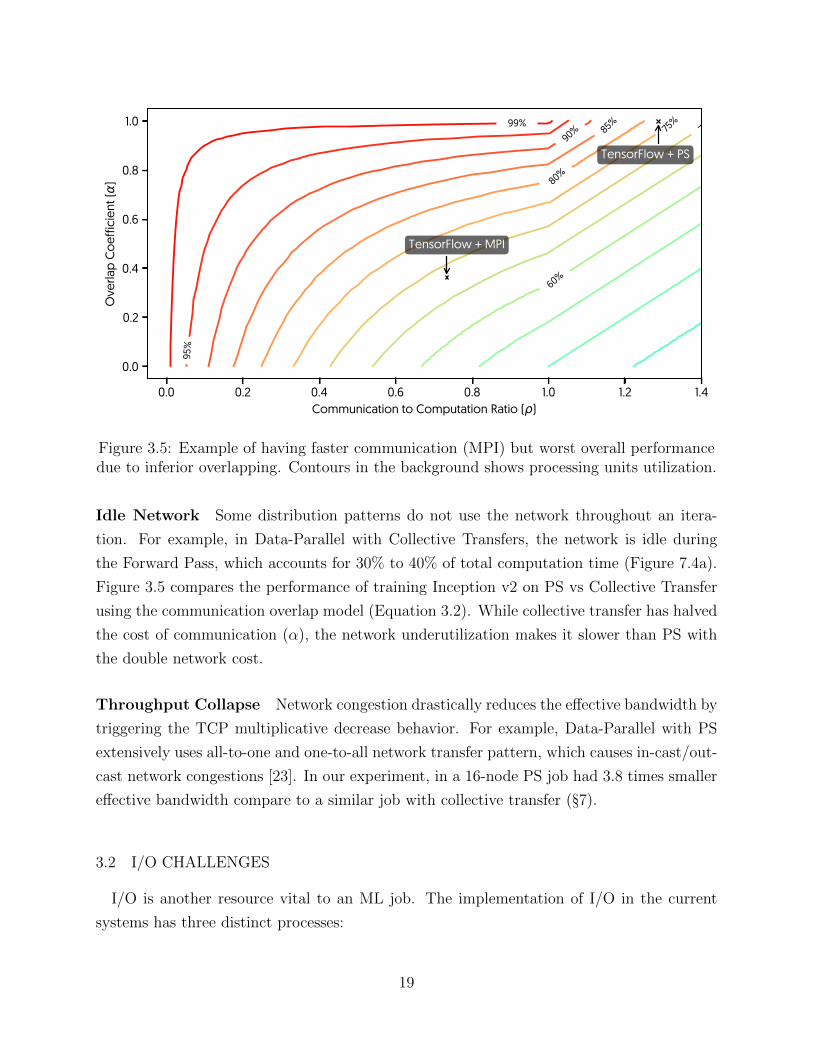
Figure 3.5: Example of having faster communication (MPI) but worst overall performancedue to inferior overlapping. Contours in the background shows processing units utilization.

Idle Network Some distribution patterns do not use the network throughout an itera-

tion. For example, in Data-Parallel with Collective Transfers, the network is idle during

the Forward Pass, which accounts for 30% to 40% of total computation time (Figure 7.4a).

Figure 3.5 compares the performance of training Inception v2 on PS vs Collective Transfer

using the communication overlap model (Equation 3.2). While collective transfer has halved

the cost of communication (α), the network underutilization makes it slower than PS with

the double network cost.

Throughput Collapse Network congestion drastically reduces the effective bandwidth by

triggering the TCP multiplicative decrease behavior. For example, Data-Parallel with PS

extensively uses all-to-one and one-to-all network transfer pattern, which causes in-cast/out-

cast network congestions [23]. In our experiment, in a 16-node PS job had 3.8 times smaller

effective bandwidth compare to a similar job with collective transfer (§7).

3.2 I/O CHALLENGES

I/O is another resource vital to an ML job. The implementation of I/O in the current

systems has three distinct processes:

19

1. Reading examples from a storage instument

2. Preprocessing examples

3. Loading the data to the accelerators

Only the third process, “loading the data to the accelerator”, is a part of the dataflow DAG

and is on the critical path. The first two processes are executed asynchronously separated

from the main training thread. As long as reading the data and preprocessing can keep up

with the iteration, I/O is not a performance bottleneck.

I/O in a distributed job is implemented in different ways:

• Offline Replication: In this design, a replication of the dataset is permanently repli-

cated on each worker. Each worker reads the data from the local disk. There is no

network activity involved in reading data.

• Remote Storage: In this design the dataset resides on remote file systems such as NFS

[91], GPFS [87], Lustre [88] or a remote file storage such as Google File Server [35] and

Hadoop Distributed File System [93]. Each worker reads the data over the network

during the training.

• Online Replication: In this design, the portion of the dataset a worker needs to process

is copied on the worker at the beginning of the job [65]. The worker reads the data

from the local storage for the duration of the training. The network is used in setting

up the job before the start of the training.

The I/O may become a bottle-neck in a job for various reasons, see below.

3.2.1 Slow Storage

If the storage through can not keep up with the pace of training, it becomes a bottleneck:

Latency +minibatch Data Size

Throughput> Iteration Time (3.5)

If the order of processing the examples in the dataset is known in advance, which is very

common in Deep Leaning jobs, the I/O requests are pipelined which hides the read latency.

In this case the storage throughput is the only factor in keeping up with the iteration time.

In other word, the storage is slow if:

minibatch Data Size

Throughput> Iteration Time (3.6)

20

if the Equation 3.6 does not hold true, in theory, the I/O is fast enough to handle the

training job.

3.2.2 Storage Underutilization

1 4 16 32 128Read Size (Samples)

14

816

3264

128

I/O

Dep

th

0% 1% 2% 3% 7%

1% 4% 14% 18% 19%

2% 7% 23% 28% 29%

3% 10% 35% 40% 52%

4% 15% 49% 54% 70%

6% 20% 64% 67% 87%

7% 25% 77% 80% 100%

AirFreight-all

1 4 16 32 128Read Size (Samples)

14

816

3264

128

I/O

Dep

th

1% 3% 9% 18% 52%

10% 20% 25% 43% 80%

17% 33% 32% 48% 84%

25% 48% 49% 59% 84%

36% 65% 64% 72% 86%

47% 82% 79% 85% 90%

57% 100% 91% 95% 100%

COCO-test

1 4 16 32 128Read Size (Samples)

14

816

3264

128

I/O

Dep

th

2% 5% 10% 18% 54%

10% 19% 26% 44% 84%

17% 32% 32% 51% 87%

26% 48% 51% 60% 87%

36% 65% 67% 74% 92%

47% 81% 82% 88% 95%

57% 97% 95% 97% 100%

COCO-train

1 4 16 32 128Read Size (Samples)

14

816

3264

128

I/O

Dep

th

2% 3% 9% 18% 52%

10% 21% 25% 44% 77%

17% 32% 31% 48% 82%

26% 48% 47% 59% 82%

36% 65% 62% 74% 84%

48% 82% 76% 88% 87%

58% 100% 88% 99% 91%

COCO-val

1 4 16 32 128Read Size (Samples)

14

816

3264

128

I/O

Dep

th

1% 2% 5% 10% 28%

5% 13% 13% 26% 60%

9% 21% 23% 33% 64%

13% 30% 43% 50% 71%

19% 40% 56% 68% 82%

25% 50% 69% 83% 93%

31% 61% 82% 95% 100%

berkeley_segmentation-test

1 4 16 32 128Read Size (Samples)

14

816

3264

128

I/O

Dep

th

0% 2% 3% 6% 21%

3% 10% 8% 16% 49%

6% 16% 15% 21% 55%

9% 24% 28% 32% 64%

13% 33% 37% 43% 77%

18% 43% 46% 52% 91%

22% 52% 53% 60% 100%

berkeley_segmentation-train

1 4 16 32 128Read Size (Samples)

14

816

3264

128

I/O

Dep

th

1% 3% 8% 16% 49%

10% 19% 23% 41% 79%

16% 30% 30% 45% 84%

25% 45% 50% 57% 84%

36% 60% 67% 72% 88%

47% 76% 80% 87% 93%

57% 91% 92% 96% 100%

flickr30k-all

1 4 16 32 128Read Size (Samples)

14

816

3264

128

I/O

Dep

th

1% 3% 8% 16% 46%

9% 18% 22% 39% 78%

16% 29% 28% 43% 83%

25% 43% 46% 55% 84%

35% 58% 62% 70% 87%

46% 73% 76% 84% 94%

56% 89% 88% 94% 100%

flickr8k-all

1 4 16 32 128Read Size (Samples)

14

816

3264

128

I/O

Dep

th

0% 1% 2% 3% 10%

2% 6% 15% 19% 25%

3% 10% 24% 32% 33%

4% 16% 35% 46% 53%

6% 23% 47% 61% 70%

9% 30% 60% 76% 87%

11% 37% 74% 91% 100%

google_house_number-test

1 4 16 32 128Read Size (Samples)

14

816

3264

128

I/O

Dep

th

0% 0% 2% 3% 6%

1% 4% 13% 19% 16%

2% 6% 21% 30% 27%

3% 10% 32% 43% 52%

4% 15% 45% 57% 69%

5% 19% 58% 73% 85%

7% 24% 71% 89% 100%

google_house_number-train

1 4 16 32 128Read Size (Samples)

14

816

3264

128

I/O

Dep

th1% 2% 6% 11% 35%

6% 15% 16% 30% 68%

11% 23% 28% 36% 72%

17% 34% 53% 53% 73%

23% 45% 70% 69% 79%

30% 55% 85% 86% 87%

37% 67% 100% 97% 94%

imagenet-train

1 4 16 32 128Read Size (Samples)

14

816

3264

128

I/O

Dep

th

1% 3% 8% 15% 42%

9% 19% 21% 37% 75%

14% 30% 30% 41% 79%

22% 43% 53% 55% 81%

31% 57% 70% 72% 86%

41% 71% 86% 85% 91%

51% 85% 100% 96% 97%

imagenet-validation

1 4 16 32 128Read Size (Samples)

14

816

3264

128

I/O

Dep

th

3% 11% 30% 51% 100%

8% 25% 46% 52% 59%

14% 28% 48% 54% 65%

26% 33% 46% 52% 55%

34% 39% 49% 52% 54%

41% 46% 50% 52% 52%

47% 50% 39% 52% 52%

youtube-8m-video-test

1 4 16 32 128Read Size (Samples)

14

816

3264

128

I/O

Dep

th

7% 21% 54% 73% 100%

18% 33% 42% 42% 50%

20% 35% 43% 44% 51%

23% 35% 40% 42% 40%

30% 37% 41% 40% 45%

34% 39% 38% 39% 42%

38% 40% 38% 40% 43%

youtube-8m-video-train

1 4 16 32 128Read Size (Samples)

14

816

3264

128

I/O

Dep

th

3% 10% 30% 49% 100%

8% 24% 44% 50% 57%

13% 27% 46% 53% 62%

24% 31% 45% 49% 54%

32% 38% 48% 52% 52%

39% 45% 49% 51% 52%

46% 50% 51% 49% 55%

youtube-8m-video-validate

0.0

0.2

0.4

0.6

0.8

1.0

0.0

0.2

0.4

0.6

0.8

1.0

0.0

0.2

0.4

0.6

0.8

1.0

0.0

0.2

0.4

0.6

0.8

1.0

0.0

0.2

0.4

0.6

0.8

1.0

0.0

0.2

0.4

0.6

0.8

1.0

0.0

0.2

0.4

0.6

0.8

1.0

0.0

0.2

0.4

0.6

0.8

1.0

0.0

0.2

0.4

0.6

0.8

1.0

0.0

0.2

0.4

0.6

0.8

1.0

0.0

0.2

0.4

0.6

0.8

1.0

0.0

0.2

0.4

0.6

0.8

1.0

0.0

0.2

0.4

0.6

0.8

1.0

0.0

0.2

0.4

0.6

0.8

1.0

0.0

0.2

0.4

0.6

0.8

1.0

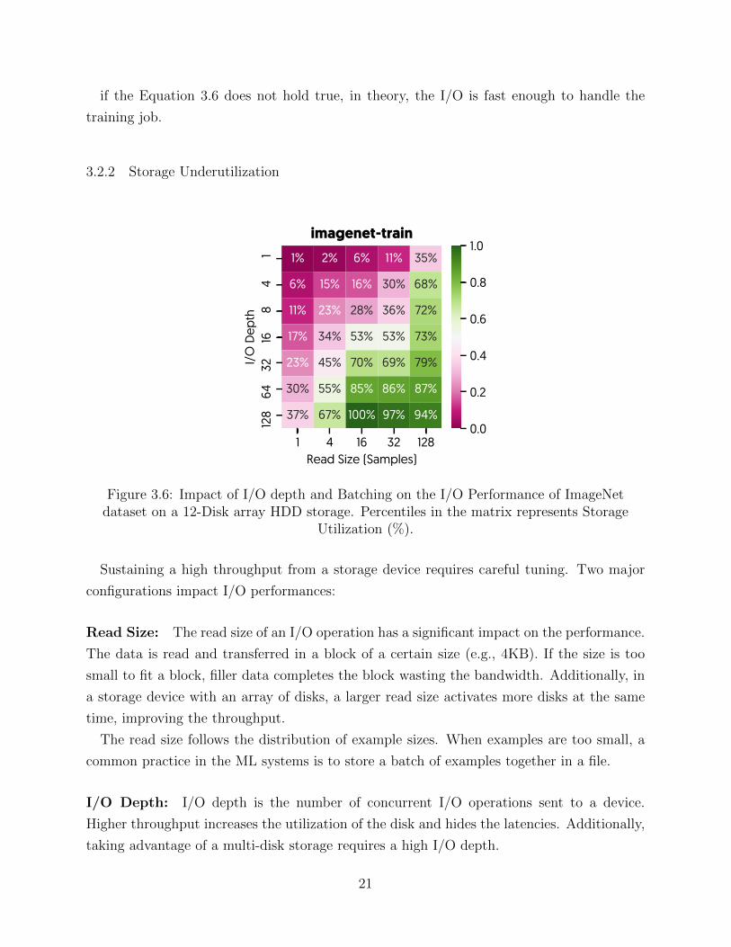
Figure 3.6: Impact of I/O depth and Batching on the I/O Performance of ImageNetdataset on a 12-Disk array HDD storage. Percentiles in the matrix represents Storage

Utilization (%).

Sustaining a high throughput from a storage device requires careful tuning. Two major

configurations impact I/O performances:

Read Size: The read size of an I/O operation has a significant impact on the performance.

The data is read and transferred in a block of a certain size (e.g., 4KB). If the size is too

small to fit a block, filler data completes the block wasting the bandwidth. Additionally, in

a storage device with an array of disks, a larger read size activates more disks at the same

time, improving the throughput.

The read size follows the distribution of example sizes. When examples are too small, a

common practice in the ML systems is to store a batch of examples together in a file.

I/O Depth: I/O depth is the number of concurrent I/O operations sent to a device.

Higher throughput increases the utilization of the disk and hides the latencies. Additionally,

taking advantage of a multi-disk storage requires a high I/O depth.

21

The I/O throughput is very sensitive to these two performance knobs. Figure 3.6 shows the

impact of these variables on the throughput of an 12-disk array reading some ML datasets.

In all cases, reading the data without batching or with I/O depth of one significantly de-

grades the throughput up to 99%. These variables are set through the application by the

developer and cannot be enforced through the operating systems or hardware. In our sur-

vey of top 10 Deep Learning jobs in MRI-DL project in NCSA [34], we have observed I/O

misconfigurations in 8 jobs.

Impact of Distribution: Achieving higher I/O throughput to serve multiple workers

requires a larger number of disks arrayed together. This increase in the number of disks

makes the I/O misconfiguration even less forgiving results in higher performance loss due to

misconfigurations.

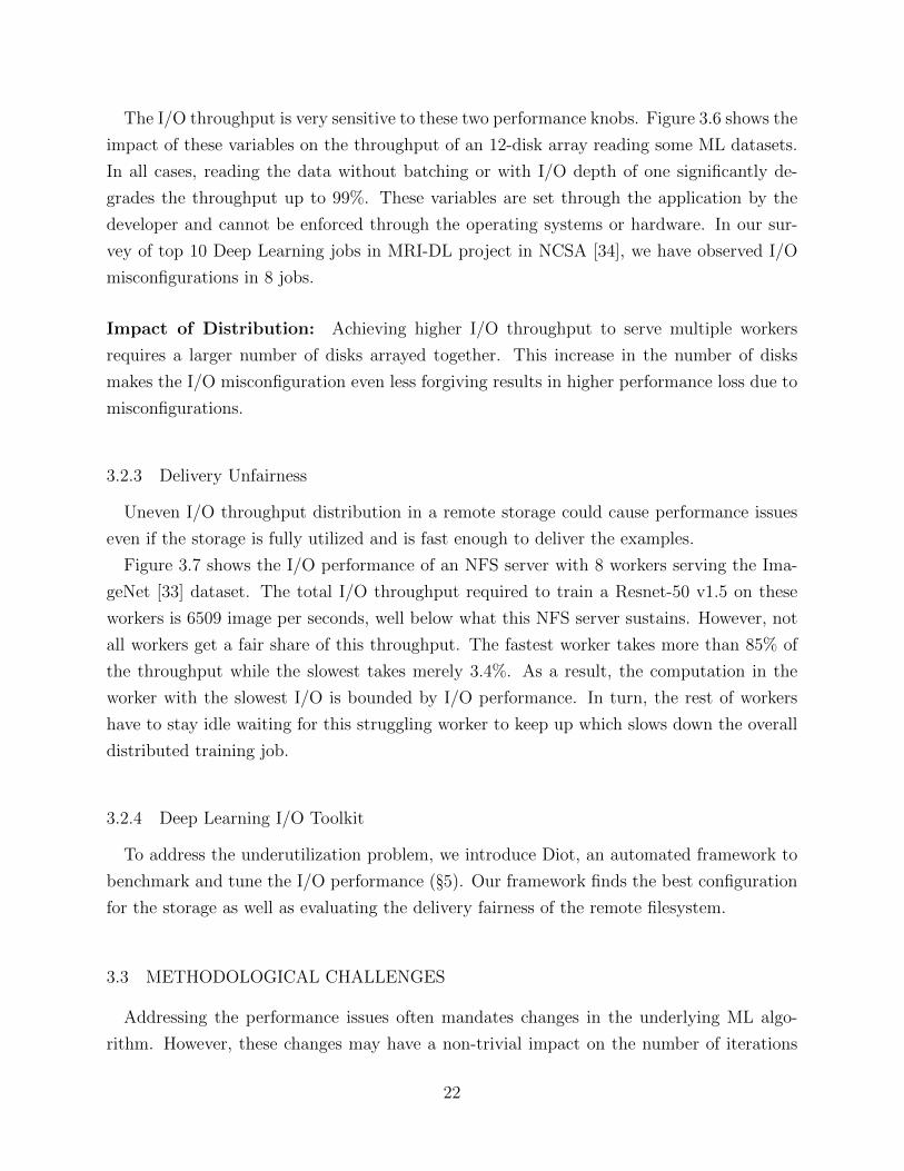
3.2.3 Delivery Unfairness

Uneven I/O throughput distribution in a remote storage could cause performance issues

even if the storage is fully utilized and is fast enough to deliver the examples.

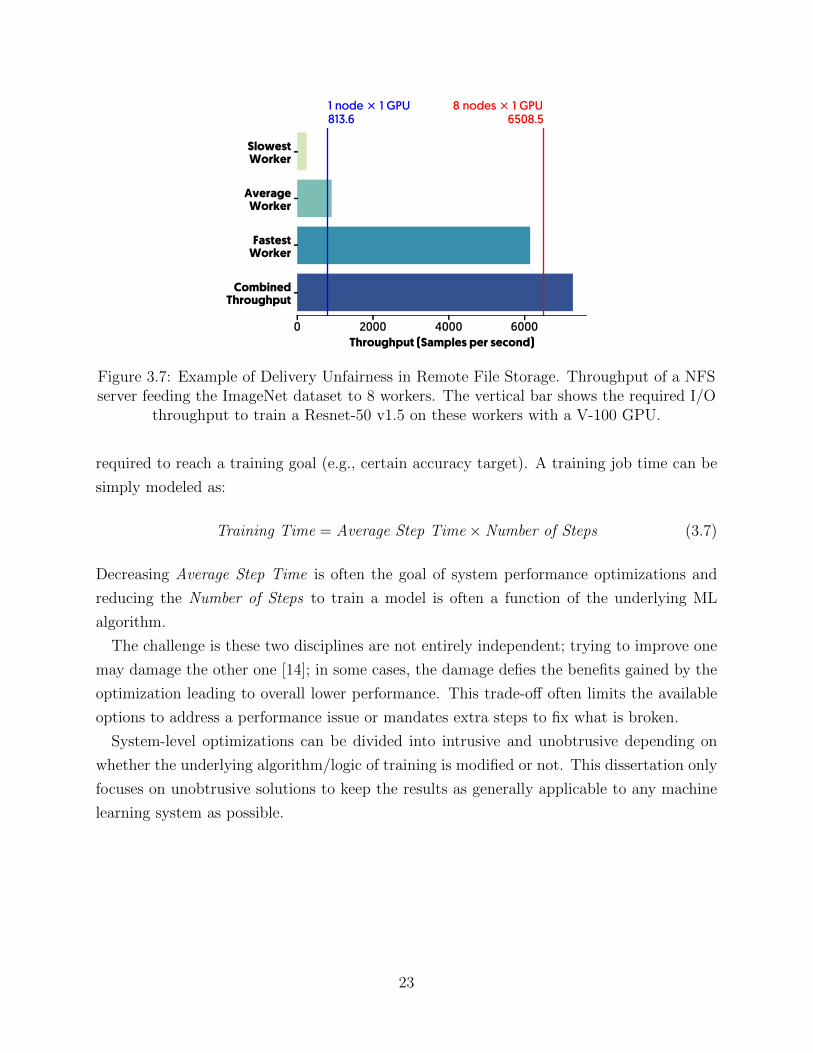
Figure 3.7 shows the I/O performance of an NFS server with 8 workers serving the Ima-

geNet [33] dataset. The total I/O throughput required to train a Resnet-50 v1.5 on these

workers is 6509 image per seconds, well below what this NFS server sustains. However, not

all workers get a fair share of this throughput. The fastest worker takes more than 85% of

the throughput while the slowest takes merely 3.4%. As a result, the computation in the

worker with the slowest I/O is bounded by I/O performance. In turn, the rest of workers

have to stay idle waiting for this struggling worker to keep up which slows down the overall

distributed training job.

3.2.4 Deep Learning I/O Toolkit

To address the underutilization problem, we introduce Diot, an automated framework to

benchmark and tune the I/O performance (§5). Our framework finds the best configuration

for the storage as well as evaluating the delivery fairness of the remote filesystem.

3.3 METHODOLOGICAL CHALLENGES

Addressing the performance issues often mandates changes in the underlying ML algo-

rithm. However, these changes may have a non-trivial impact on the number of iterations

22

0 2000 4000 6000Throughput (Samples per second)

SlowestWorker

AverageWorker

FastestWorker

CombinedThroughput

8 nodes × 1 GPU6508.5

1 node × 1 GPU813.6

Figure 3.7: Example of Delivery Unfairness in Remote File Storage. Throughput of a NFSserver feeding the ImageNet dataset to 8 workers. The vertical bar shows the required I/O

throughput to train a Resnet-50 v1.5 on these workers with a V-100 GPU.

required to reach a training goal (e.g., certain accuracy target). A training job time can be

simply modeled as:

Training Time = Average Step Time× Number of Steps (3.7)

Decreasing Average Step Time is often the goal of system performance optimizations and

reducing the Number of Steps to train a model is often a function of the underlying ML

algorithm.

The challenge is these two disciplines are not entirely independent; trying to improve one

may damage the other one [14]; in some cases, the damage defies the benefits gained by the

optimization leading to overall lower performance. This trade-off often limits the available

options to address a performance issue or mandates extra steps to fix what is broken.

System-level optimizations can be divided into intrusive and unobtrusive depending on

whether the underlying algorithm/logic of training is modified or not. This dissertation only

focuses on unobtrusive solutions to keep the results as generally applicable to any machine

learning system as possible.

23

CHAPTER 4: PERFORMANCE OBSERVABILITY IN DISTRIBUTEDMACHINE LEARNING

“It is a capital mistake to theorize before one has data.Insensibly one begins to twist facts to suit theories, insteadof theories to suit facts.”

Arthur Conan Doylein The Adventures of Sherlock Holmes

The promise of Systems performance is to study any physical entity or software compo-

nents affecting the performance. This study not only requires a disciplined methodology but

relies heavily on specialized tools to collect performance events. These events happen on

different entities at different time. There are two ways to collect these events:

Profiling records the events bar the timing and order of the event, which helps to find

load imbalance in the system and excessive resource uses.

Tracing records the event with timestamps and/or ordering of the event, which helps to

examine timing issues in the system. In exchange, tracing has a larger memory and overhead

footprint.

For a distributed job, capturing events additionally requires coordination among nodes,

dealing with network overhead caused by coordinations, and accurate deduction order of

internetwork events

In this chapter, we discuss our work in filling the gap in tracing and profiling toolkits

for distributed ML jobs. First, we explain our work to scale out the ML execution tracing

specially capturing network events. Later, we explain the design of a new visualization

tailored for performance analysis of distributed ML jobs. Lastly, we expand our effort to

fulfill the shortcomings of tracing and profiling ML jobs in the production.

Our work in tracing is implemented on TensorFlow and publicly available. Throughout

this chapter, TensorFlow conventions are extensively used.

4.1 DISTRIBUTED TRACING

Tracing ops in a dataflow DAG is quite straightforward. It can be done simply by record

the time of start and end of each op. However, a vast majority of ops do not execute in

the main process but trigger events in different execution environment outside of the main

process. For example:

24

Execution

SetLogging(True)

Iteration

Logging

SetLogging(False)

RetrieveLogs()

ClearLogs()

Timeline

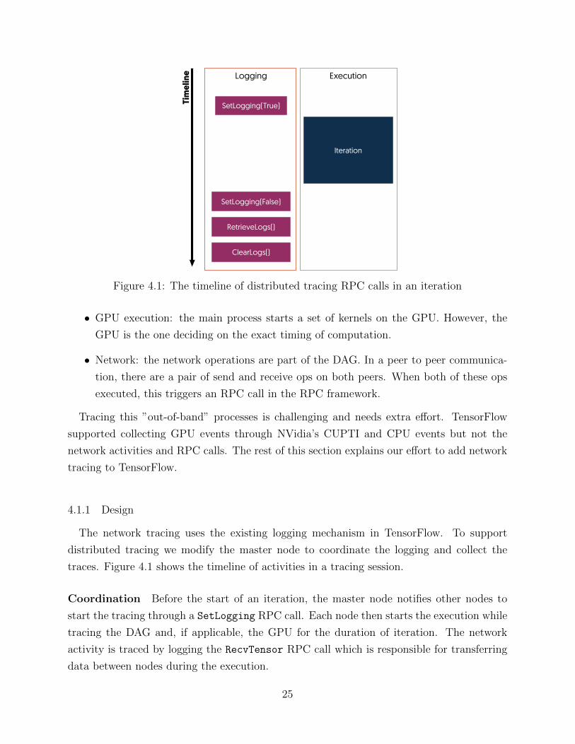
Figure 4.1: The timeline of distributed tracing RPC calls in an iteration

• GPU execution: the main process starts a set of kernels on the GPU. However, the

GPU is the one deciding on the exact timing of computation.

• Network: the network operations are part of the DAG. In a peer to peer communica-

tion, there are a pair of send and receive ops on both peers. When both of these ops

executed, this triggers an RPC call in the RPC framework.

Tracing this ”out-of-band” processes is challenging and needs extra effort. TensorFlow

supported collecting GPU events through NVidia’s CUPTI and CPU events but not the

network activities and RPC calls. The rest of this section explains our effort to add network

tracing to TensorFlow.

4.1.1 Design

The network tracing uses the existing logging mechanism in TensorFlow. To support

distributed tracing we modify the master node to coordinate the logging and collect the

traces. Figure 4.1 shows the timeline of activities in a tracing session.

Coordination Before the start of an iteration, the master node notifies other nodes to

start the tracing through a SetLogging RPC call. Each node then starts the execution while

tracing the DAG and, if applicable, the GPU for the duration of iteration. The network

activity is traced by logging the RecvTensor RPC call which is responsible for transferring

data between nodes during the execution.

25

Managing the Network Overhead Tracing data is not immediately collected over the

network and is stored locally during the iteration. When the iteration finishes, the master

turns off the logging through another SetLogging RPC call. Then the logs are collected by

an RetrieveLogs RPC call to each node followed by a ClearLogs call to remove the local

storage of the logs.

Even though this collection phase between iterations significantly slowdowns the overall

job time; it does not have a noticeable impact on the execution of iteration.

4.1.2 Implementation and Availability

We have implemented the network tracing module on TensorFlow. The implementation

adds the gRPC RPC events to the TF standard tracing format. The network tracing module

is 115 lines of C++ code1 and has been a part of standard TensorFlow from v1.5.0.

4.2 VISUALIZATION

Visualization is an effective way to examine a large quantity of data and find patterns and

correlations in the traces, which may be difficult to achieve through other means [39].

A distributed training job trace commonly contains a sizable number of events, which

makes a visualization tool a necessity for the performance analysis of distributed jobs. For

example, a 4-worker training of Inception V3 [99] contains 8937 events.

While there are many visualizations specifically design for ML performance analysis pur-

poses, there are two tools specifically designed to visualize TensorFlow runtime traces. Ten-

sorFlow includes a tool to convert traces into Chrome Tracing Format which is visualized

with Google Chrome internal tracer. Since this tool has not been designed for ML jobs, it

does not retain much essential information in the tracing. For example, this visualization

discards the network activity details such as size, source, and destination the transfer, and

the other metadata. TensorBoard [18] includes a visualization of tracing data in a graph

format where each node represents an op and is colored proportional to its elapsed time.

This visualization discards the timing of visualization, implicitly converting the tracing data

to a profiling data.

1https://github.com/tensorflow/tensorflow/pull/14604

26

4.2.1 Design

We design our system based on Shneiderman’s principle [92], “Overview first, zoom and

filter, then details-on-demand”. Our visualization has implemented six out of seven infor-

mation visualization tasks:

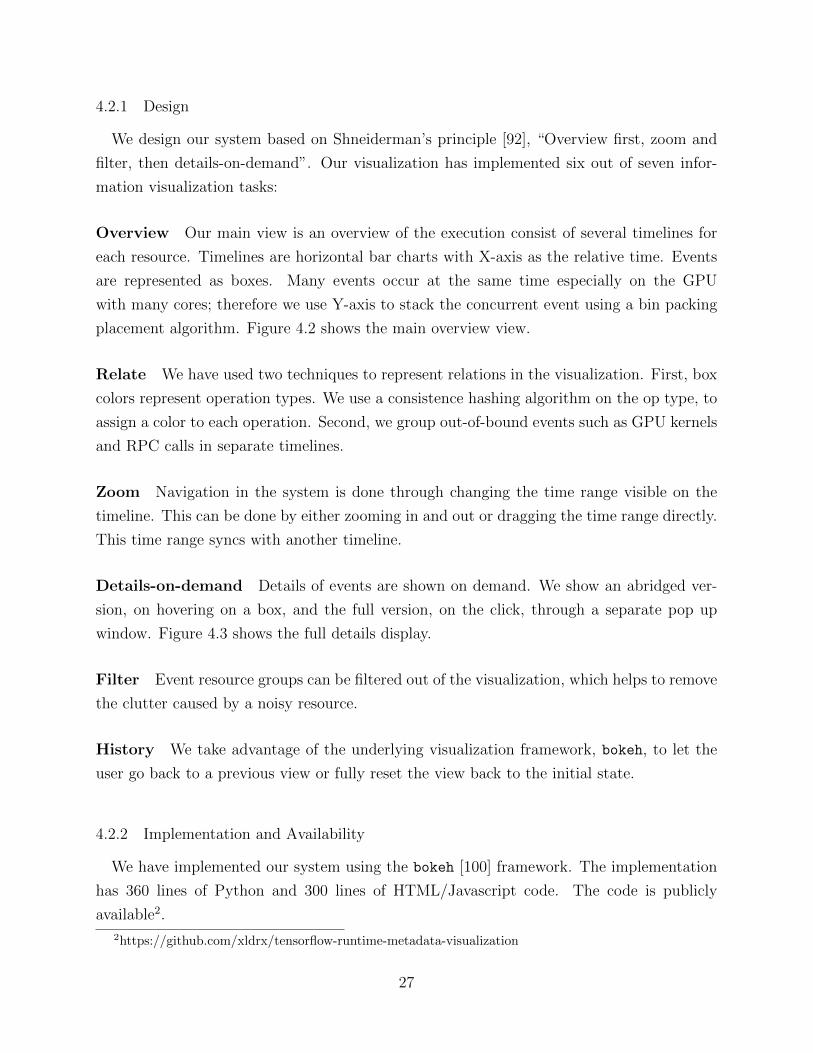
Overview Our main view is an overview of the execution consist of several timelines for

each resource. Timelines are horizontal bar charts with X-axis as the relative time. Events

are represented as boxes. Many events occur at the same time especially on the GPU

with many cores; therefore we use Y-axis to stack the concurrent event using a bin packing

placement algorithm. Figure 4.2 shows the main overview view.

Relate We have used two techniques to represent relations in the visualization. First, box

colors represent operation types. We use a consistence hashing algorithm on the op type, to

assign a color to each operation. Second, we group out-of-bound events such as GPU kernels

and RPC calls in separate timelines.

Zoom Navigation in the system is done through changing the time range visible on the

timeline. This can be done by either zooming in and out or dragging the time range directly.

This time range syncs with another timeline.

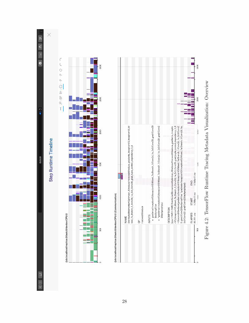
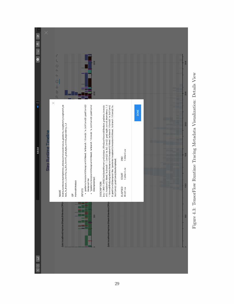
Details-on-demand Details of events are shown on demand. We show an abridged ver-

sion, on hovering on a box, and the full version, on the click, through a separate pop up

window. Figure 4.3 shows the full details display.

Filter Event resource groups can be filtered out of the visualization, which helps to remove

the clutter caused by a noisy resource.

History We take advantage of the underlying visualization framework, bokeh, to let the

user go back to a previous view or fully reset the view back to the initial state.

4.2.2 Implementation and Availability

We have implemented our system using the bokeh [100] framework. The implementation

has 360 lines of Python and 300 lines of HTML/Javascript code. The code is publicly

available2.

2https://github.com/xldrx/tensorflow-runtime-metadata-visualization

27

Fig

ure

4.2:

Ten

sorF

low

Runti

me

Tra

cing

Met

adat

aV

isual

izat

ion:

Ove

rvie

w

28

Fig

ure

4.3:

Ten

sorF

low

Runti

me

Tra

cing

Met

adat

aV

isual

izat

ion:

Det

ails

Vie

w

29

4.3 TRACING IN PRODUCTION

The growing popularity of Deep Neural Networks (DNN) within the mainstream [94]

has had a rapid transformative effect on clusters and data centers. DNN training jobs

are becoming one of the largest tenants within clusters, and often take hours to weeks to

complete, and even a slight performance improvement can save substantial runtime costs.

Despite this fact, the DNN specific performance tuning tools are yet to keep up with the

needs of the new changes in production environments.

On the one hand, the existing application-agnostic resource-level tools such as top, Nvidia

Nsight (for GPU utilization), IPM (for MPI network monitoring) are too limited to predict

or explain the behavior and performance of a job accurately. In DNN applications, there

exists a complex relationship among resources. Even though measuring coarse metrics such

as bandwidth, latency, and GPU/CPU utilization can draw an overall picture of cluster

performance, these metrics are not easily translatable to application-level metrics and do

not provide actionable insights on how to handle performance bottlenecks.

On the other hand, the shortlist of application-aware tools, such as MLModelScope [30],

TensorBoard [18], and tf.RunOptions 3, while able to provide actionable insights, are mainly

designed for the need of application developers and are not intended for production use. Such

tools require substantial modification to applications and early planning as to what, when,

and how data should be collected.

We introduce tensorflow-tracer to fill the gap between these two classes of performance

tuning tools. The tensorflow-tracer addresses the following technical challenges:

• Collecting the application-level runtime metrics, such as the timing of each operation or the

total iteration time, required application source code modification. To avoid application-

level modification, tensorflow-tracer monkeypatches the tensorflow library at the

system level allowing on-demand application tracing.

• Collecting some metrics is expensive and has a significant overhead on the runtime.

tensorflow-tracer treats metrics differently; it collects low-overhead metrics automati-

cally, while expensive ones are collected on demand through an admin interface.

• There is no easy way to exchange runtime metrics among users and admins — our system

facilities this through a portable file format and supporting tools to explore these metrics

offline.

3https://www.tensorflow.org/api_docs/python/tf/RunOptions

30

TensorFlow Application

tensorflow-tracer

TensorFlow

REST/Web InterfaceMonkeyPatching

Data Management

Admin

CLI

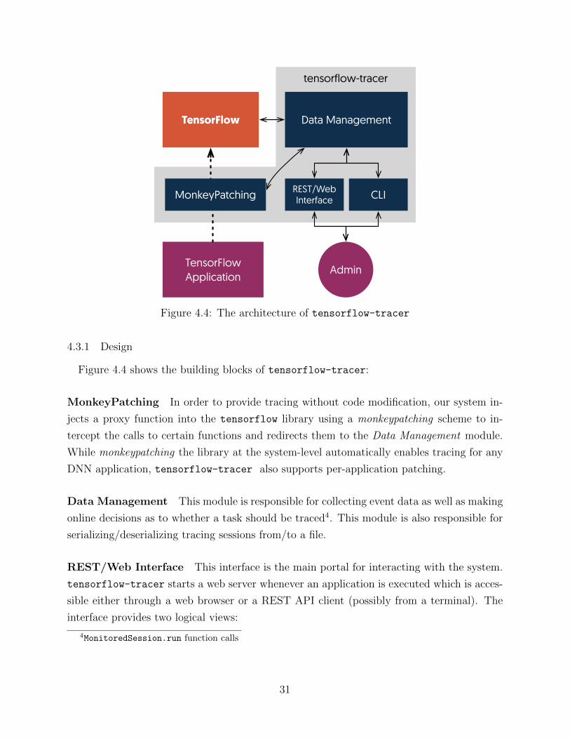
Figure 4.4: The architecture of tensorflow-tracer

4.3.1 Design

Figure 4.4 shows the building blocks of tensorflow-tracer:

MonkeyPatching In order to provide tracing without code modification, our system in-

jects a proxy function into the tensorflow library using a monkeypatching scheme to in-

tercept the calls to certain functions and redirects them to the Data Management module.

While monkeypatching the library at the system-level automatically enables tracing for any

DNN application, tensorflow-tracer also supports per-application patching.

Data Management This module is responsible for collecting event data as well as making

online decisions as to whether a task should be traced4. This module is also responsible for

serializing/deserializing tracing sessions from/to a file.

REST/Web Interface This interface is the main portal for interacting with the system.

tensorflow-tracer starts a web server whenever an application is executed which is acces-

sible either through a web browser or a REST API client (possibly from a terminal). The

interface provides two logical views:

4MonitoredSession.run function calls

31

Fig

ure

4.5:

The

mai

nw

ebin

terf

ace

oftensorflow-tracer.

Eac

hen

try

repre

sents

ase

par

ate

task

inth

eD

NN

sess

ion.

32

Fig

ure

4.6:

The

tim

elin

ein

terf

ace

pro

vid

esdet

ails

ofth

eex

ecuti

onof

one

iter

atio

nst

ep.

Eac

hb

oxre

pre

sent

anop

erat

ion

inth

eD

ataF

low

DA

G.

Ther

eis

ati

mel

ine

for

ever

yre

sourc

eson

each

mac

hin

e.T

he

trac

eis

collec

ted

from

nextframesv2p[1

0]m

odel

intensor2tensor

libra

ry[1

06].

33

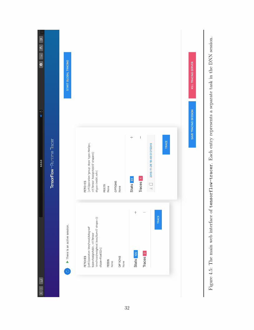
1. Main Interface shows the list of tasks and their associated profiling/tracing data. This

interface allows request tracing. (Figure 4.5)

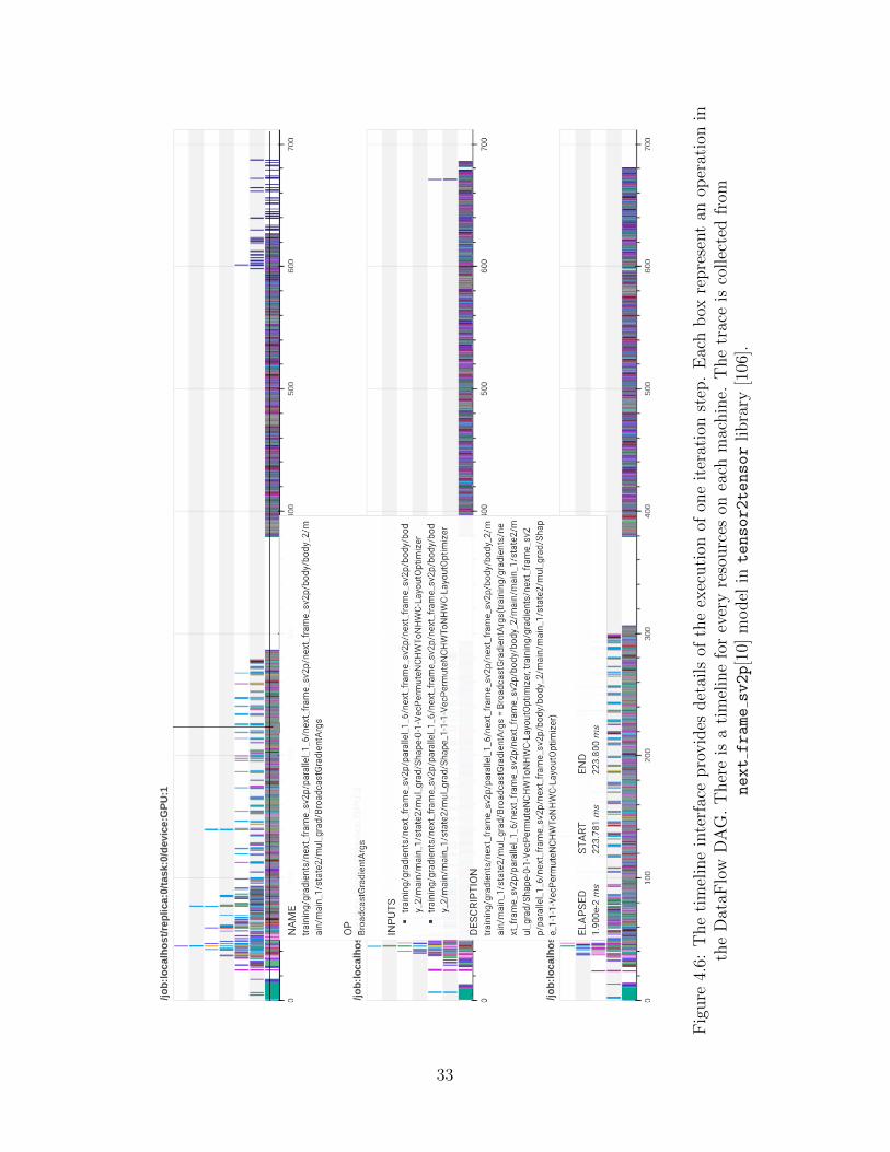
2. Timeline Interface visualizes an instance of a task trace as a series of timelines, one

for every resource (e.g., CPU, GPU, Network Interface) on each machine. Each box

represents operation in the DataFlow DAG of DNN application. (Figure 4.6)

CLI It loads a tracing session offline and enables exploring through a web interface.

4.3.2 tensorflow-tracer in action

Overhead We observe no performance hit on collecting low-overhead metrics such as it-

eration times, ‘session.run‘ call names and frequencies. We observe less than 3% runtime

overhead to iteration time when individual operations in a call are traced. CPU Memory

requirements varies for different models. For example: an Inception v3 [99] trace consumes

718KB while next frame sv2p [10] consumes 2.4MB.

Case Study We have used tensorflow-tracer on different workloads to find the perfor-

mance issues on application, framework, and infrastructure level. This is the main tool we

used in §6, §7 and §7.8.

4.3.3 Implementation and Availability

We have implemented tensorflow-tracer in Python. The implementation is Python

1100 LOC and 800 LOC of HTML/JavaScript. it is publicly available under Apache-2.0

license5. It supports native TensorFlow [1], Horovod [90], and IBM PowerAI [25] applica-

tions.

The correctness of the tensorflow-tracer’s distributed traces relies on the precision of

the clocks on the different machines. Currently, it relies on external sources to synchronize

the clocks.

5https://github.com/xldrx/tensorflow-tracer

34

CHAPTER 5: I/O IN DISTRIBUTED MACHINE LEARNING

Large scale computation in deep learning training demands the loading of a high volume

of data. Consequently, I/O has become an integral part of an ML training iteration with

a critical impact on the overall performance. Ever growing computational demand of ML

workloads not only has introduced accelerators in enterprise clusters but also has evolved

the storage infrastructure from off-the-shelf local disks to highly parallel storage systems.

On the software side, frameworks like Tensorflow and Pytorch have harness next-generation

storage system by evolving their I/O pipeline with optimizations such as batching and paral-

lelism. However, the behavior and efficiency of these optimizations are controlled by multiple

I/O knobs, such as the number of concurrent I/O operations (IOP) sent to a storage device

and the read size of each IOP. In the absence of a sufficiently comprehensive understanding

of the effect of these knobs on the I/O throughput, the task of tuning these settings is wholly

left to end-users in existing systems.

In this chapter, we attempt to provide an extensive experimental study on the effects of

I/O tuning on modern ML systems. In order to achieve this goal, we have implemented Diot,

a Deep Learning I/O toolkit, to automate and accelerate I/O benchmarking on distributed

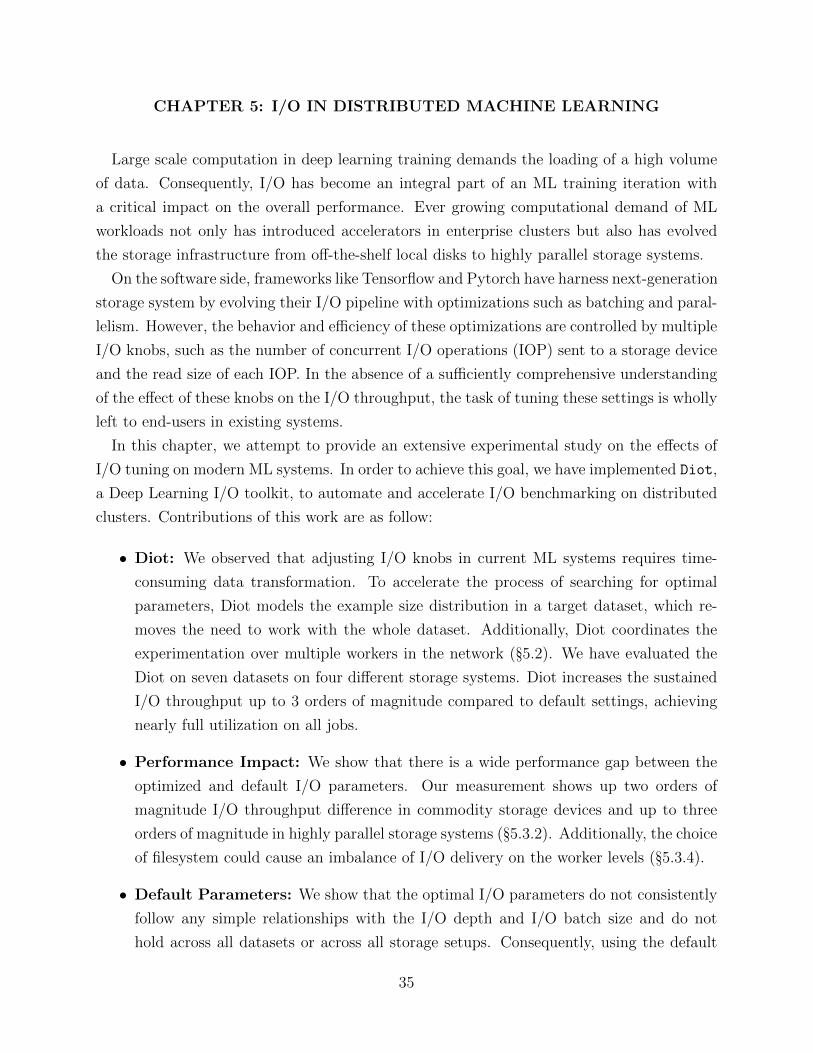
clusters. Contributions of this work are as follow:

• Diot: We observed that adjusting I/O knobs in current ML systems requires time-

consuming data transformation. To accelerate the process of searching for optimal

parameters, Diot models the example size distribution in a target dataset, which re-

moves the need to work with the whole dataset. Additionally, Diot coordinates the

experimentation over multiple workers in the network (§5.2). We have evaluated the

Diot on seven datasets on four different storage systems. Diot increases the sustained

I/O throughput up to 3 orders of magnitude compared to default settings, achieving

nearly full utilization on all jobs.

• Performance Impact: We show that there is a wide performance gap between the

optimized and default I/O parameters. Our measurement shows up two orders of

magnitude I/O throughput difference in commodity storage devices and up to three

orders of magnitude in highly parallel storage systems (§5.3.2). Additionally, the choice

of filesystem could cause an imbalance of I/O delivery on the worker levels (§5.3.4).

• Default Parameters: We show that the optimal I/O parameters do not consistently

follow any simple relationships with the I/O depth and I/O batch size and do not

hold across all datasets or across all storage setups. Consequently, using the default

35

800.0B 10.9KB 21.0KB 31.1KB

Median=4.5KBAirFreight (all)

749.0B 63.8KB 126.9KB 190.0KB

Median=7.9KBgoogle_house_number (test)

671.0B 25.7KB 50.7KB 75.7KB

Median=6.1KBgoogle_house_number (train)

23.1KB 53.3KB 83.4KB 113.6KB

Median=70.1KBberkeley_segmentation (train)

30.1KB 59.4KB 88.8KB 118.2KB

Median=75.0KBberkeley_segmentation (test)

508.0B 118.5KB 236.4KB 354.4KB

Median=104.8KBimagenet (train)

986.0B 109.6KB 218.2KB 326.9KB

Median=123.1KBimagenet (validation)

20.8KB 95.7KB 170.6KB 245.5KB

Median=130.0KBflickr8k (all)

10.4KB 87.2KB 164.0KB 240.8KB

Median=132.7KBflickr30k (all)

3.6KB 115.0KB 226.3KB 337.7KB

Median=150.9KBCOCO (test)

4.9KB 115.6KB 226.4KB 337.1KB

Median=151.1KBCOCO (train)

8.7KB 115.7KB 222.8KB 329.9KB

Median=150.3KBCOCO (val)

1.1MB 1.2MB 1.3MB 1.5MB

Median=1.3MByoutube-8m-video (test)

4.1MB 4.4MB 4.6MB 4.8MB

Median=4.5MByoutube-8m-video (train)

1.0MB 1.2MB 1.3MB 1.5MB

Median=1.3MByoutube-8m-video (validate)

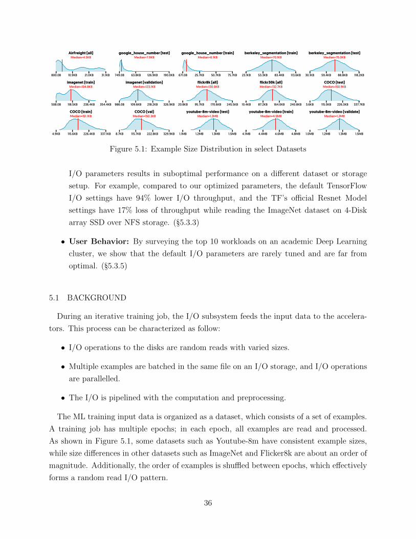
Figure 5.1: Example Size Distribution in select Datasets

I/O parameters results in suboptimal performance on a different dataset or storage

setup. For example, compared to our optimized parameters, the default TensorFlow

I/O settings have 94% lower I/O throughput, and the TF’s official Resnet Model

settings have 17% loss of throughput while reading the ImageNet dataset on 4-Disk

array SSD over NFS storage. (§5.3.3)

• User Behavior: By surveying the top 10 workloads on an academic Deep Learning

cluster, we show that the default I/O parameters are rarely tuned and are far from

optimal. (§5.3.5)

5.1 BACKGROUND

During an iterative training job, the I/O subsystem feeds the input data to the accelera-

tors. This process can be characterized as follow:

• I/O operations to the disks are random reads with varied sizes.

• Multiple examples are batched in the same file on an I/O storage, and I/O operations

are parallelled.

• The I/O is pipelined with the computation and preprocessing.

The ML training input data is organized as a dataset, which consists of a set of examples.

A training job has multiple epochs; in each epoch, all examples are read and processed.

As shown in Figure 5.1, some datasets such as Youtube-8m have consistent example sizes,

while size differences in other datasets such as ImageNet and Flicker8k are about an order of

magnitude. Additionally, the order of examples is shuffled between epochs, which effectively

forms a random read I/O pattern.

36

After an example is read from an I/O storage, it may go through a preprocessing phase,

including transformation (e.g., resizing images [49], or “Fourier transform” on speech [7]) and

augmentation (e.g., cropping or adding noise). Later, the preprocessed example is loaded on

the accelerator and processed by the ML model.

In the current modern ML systems, these phases, 1) reading from an I/O storage, 2)

preprocessing examples, and 3) computation on an accelerator are pipelined to improve

the computation utilization (Figure 5.2). The intended behavior of the I/O pipelining is

to make the computation the only bounding resource. However, if the I/O storage is too

slow to deliver the examples, it becomes the bottleneck in the job wasting computational

resources.

5.1.1 I/O Optimizations

There are two common practices to improve the I/O throughput in the current imple-

mentations: Parallelization and Batching. Both optimizations are essential to achieving

high I/O throughput and are controlled by performance knobs: I/O depth and batch size,

respectively.

Parallelization: In parallelization, multiple I/O requests are sent to storage simultane-

ously, which in turn increases the chance of activating more disks at the same time in disk

arrays and allows better scheduling and pipelining at disk-level. The number of concurrent

I/O requests is referred to as I/O depth. While increasing I/O depth is shown to improve the

I/O performance, huge I/O depth could cause contention in the storage and kernel, which

in turn hurts the I/O performance.

Batching: In batching, examples are grouped to form larger blocks; blocks are accessed

randomly, but examples in a block are read sequentially and get shuffled in the memory

afterward. This optimization improves the I/O throughput and effectively converts the I/O

pattern from the random read to the sequential read. Additionally, it avoids the I/O channel

underutilization of small I/O requests.

Current ML systems achieve batching through merging dataset files into larger sequence

files. This transformation is statically done prior to the training, and depending on the

dataset size could take a long time to finish.

37

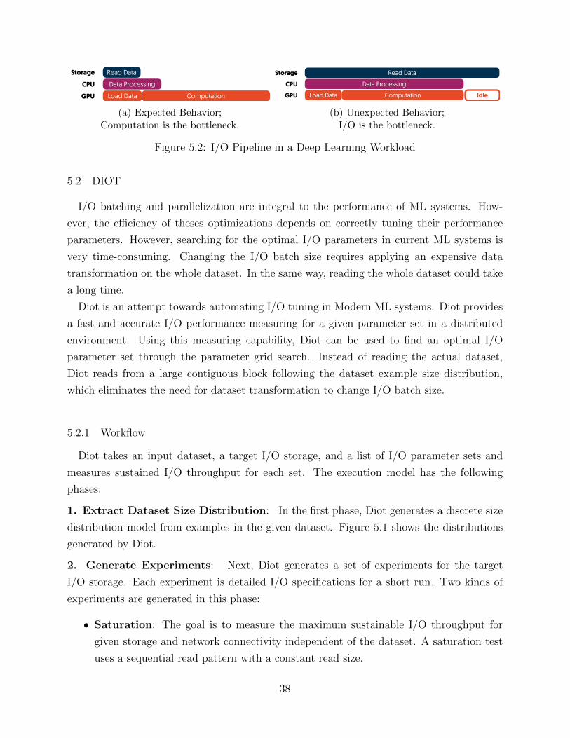
Read Data

Data Processing

Load Data Computation

Storage

CPU

GPU

(a) Expected Behavior;Computation is the bottleneck.

Read Data

Data Processing

Load Data Computation Idle

Storage

CPU

GPU

(b) Unexpected Behavior;I/O is the bottleneck.

Figure 5.2: I/O Pipeline in a Deep Learning Workload

5.2 DIOT

I/O batching and parallelization are integral to the performance of ML systems. How-

ever, the efficiency of theses optimizations depends on correctly tuning their performance

parameters. However, searching for the optimal I/O parameters in current ML systems is

very time-consuming. Changing the I/O batch size requires applying an expensive data

transformation on the whole dataset. In the same way, reading the whole dataset could take

a long time.

Diot is an attempt towards automating I/O tuning in Modern ML systems. Diot provides

a fast and accurate I/O performance measuring for a given parameter set in a distributed

environment. Using this measuring capability, Diot can be used to find an optimal I/O

parameter set through the parameter grid search. Instead of reading the actual dataset,

Diot reads from a large contiguous block following the dataset example size distribution,

which eliminates the need for dataset transformation to change I/O batch size.

5.2.1 Workflow

Diot takes an input dataset, a target I/O storage, and a list of I/O parameter sets and

measures sustained I/O throughput for each set. The execution model has the following

phases:

1. Extract Dataset Size Distribution: In the first phase, Diot generates a discrete size

distribution model from examples in the given dataset. Figure 5.1 shows the distributions

generated by Diot.

2. Generate Experiments: Next, Diot generates a set of experiments for the target

I/O storage. Each experiment is detailed I/O specifications for a short run. Two kinds of

experiments are generated in this phase:

• Saturation: The goal is to measure the maximum sustainable I/O throughput for

given storage and network connectivity independent of the dataset. A saturation test

uses a sequential read pattern with a constant read size.

38

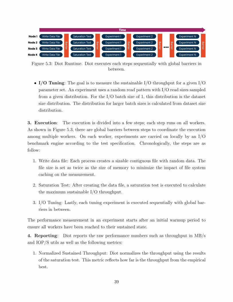
Write Data File

Write Data File

Write Data File

Write Data File

Barrier

Node 1

Node 2

Node 3

Node 4

Saturation Test

Saturation Test

Saturation Test

Saturation Test

Barrier

Experiment 1

Experiment 1

Experiment 1

Experiment 1

Barrier

Experiment 2

Experiment 2

Experiment 2

Experiment 2

Barrier

Experiment N

Experiment N

Experiment N

Experiment N

Barrier

Barrier…

Time

Figure 5.3: Diot Runtime. Diot executes each steps sequentially with global barriers inbetween.

• I/O Tuning: The goal is to measure the sustainable I/O throughput for a given I/O

parameter set. An experiment uses a random read pattern with I/O read sizes sampled

from a given distribution. For the I/O batch size of 1, this distribution is the dataset

size distribution. The distribution for larger batch sizes is calculated from dataset size

distribution.

3. Execution: The execution is divided into a few steps; each step runs on all workers.

As shown in Figure 5.3, there are global barriers between steps to coordinate the execution

among multiple workers. On each worker, experiments are carried on locally by an I/O

benchmark engine according to the test specification. Chronologically, the steps are as

follow:

1. Write data file: Each process creates a sizable contiguous file with random data. The

file size is set as twice as the size of memory to minimize the impact of file system

caching on the measurement.

2. Saturation Test: After creating the data file, a saturation test is executed to calculate

the maximum sustainable I/O throughput.

3. I/O Tuning: Lastly, each tuning experiment is executed sequentially with global bar-

riers in between.

The performance measurement in an experiment starts after an initial warmup period to

ensure all workers have been reached to their sustained state.

4. Reporting: Diot reports the raw performance numbers such as throughput in MB/s

and IOP/S utils as well as the following metrics:

1. Normalized Sustained Throughput: Diot normalizes the throughput using the results

of the saturation test. This metric reflects how far is the throughput from the empirical

best.

39

2. Example per Seconds: Diot also reports the throughput in terms of the number of

examples per second. This metric is particularly is useful when it is used with compu-

tation performance metrics in ML training.

5.2.2 Implementation

Diot is implemented in Python (900 LOC) and is publicly available at https://github.

com/xldrx/diot under GPL-3 open-source license. The implementation uses OpenMPI [38]

to spawn local processes and global barrier implementation. It also uses fio[9] as the local

I/O benchmark engine.

5.3 EXPERIMENTAL STUDY

We have conducted an experimental study on the effect of parameter tuning on I/O

throughput. More specifically, we try to answer the following questions:

• What is the performance gap between the best and the worst I/O parameters?

• Do optimized parameters hold across all datasets or storage setups?

• What is the impact of a distributed filesystem?

• How well are I/O parameters tuned in real applications?

5.3.1 Setup

We have used Diot to study on the effects of I/O tuning on modern ML systems. This

experimental study uses eight ML datasets: AirFreight [73], Berkley Segmentation [71],

Flickr8k, Flickr30k [84], Google Street View House Numbers [78], ImageNet [33], and YouTube

8m [2].

Four different storages on two clusters have been evaluated: (1) Single Disk NVMe SSD,

(2) 4-Disk Array NVMe SSD, and (3) 12-Disk SATA HDD on NCSA Hal Cluster [34] shared

through an NFSv4 remote filesystem using Infiniband 2-port EDR network. (4) a 60-Disk

Array SATA HDD on UIUC Campus Cluster [79] shared through a GPFS distributed filesys-

tem using Infiniband 2-port FDR network.

We explore two I/O parameters: I/O Batch Size with search space of {1, 4, 8, 16, 32, 128},and I/O Depth with search space of {1, 4, 8, 16, 32, 64, 128}. Using these ranges, we could

40

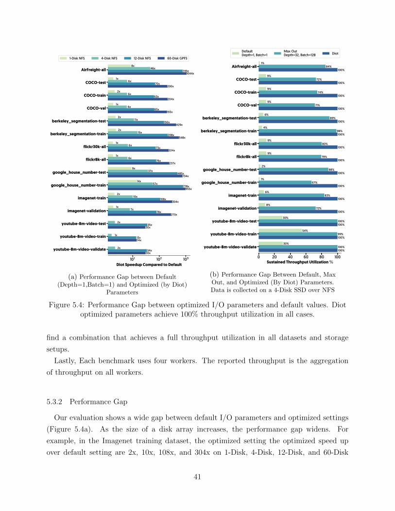
101 102 103

Diot Speedup Compared to Default

AirFreight-all

COCO-test

COCO-train

COCO-val

berkeley_segmentation-test

berkeley_segmentation-train

flickr30k-all

flickr8k-all

google_house_number-test

google_house_number-train

imagenet-train

imagenet-validation

youtube-8m-video-test

youtube-8m-video-train

youtube-8m-video-validate

8x

1x

2x

1x

2x

2x

1x

1x

9x

14x

2x

1x

46x

6x

6x

6x

11x

15x

6x

6x

37x

57x

10x

7x

2x

1x

2x

745x

70x

63x

65x

150x

208x

73x

76x

485x

778x

108x

78x

35x

13x

34x

1044x

200x

204x

193x

429x

548x

224x

237x

734x

955x

304x

273x

30x

14x

30x

1-Disk NFS 4-Disk NFS 12-Disk NFS 60-Disk GPFS

(a) Performance Gap between Default(Depth=1,Batch=1) and Optimized (by Diot)

Parameters

0 20 40 60 80 100Sustained Throughput Utilization %

AirFreight-all

COCO-test

COCO-train

COCO-val

berkeley_segmentation-test

berkeley_segmentation-train

flickr30k-all

flickr8k-all

google_house_number-test

google_house_number-train

imagenet-train

imagenet-validation

youtube-8m-video-test

youtube-8m-video-train

youtube-8m-video-validate

1%

9%

9%

9%

6%

4%

9%

9%

2%

1%

6%

8%

30%

54%

30%

84%

72%

74%

71%

89%

98%

80%

79%

88%

67%

83%

72%

100%

99%

100%

100%

100%

100%

100%

100%

100%

100%

100%

100%

100%

100%

100%

100%

100%

100%

DefaultDepth=1, Batch=1

Max OutDepth=32, Batch=128 Diot

(b) Performance Gap Between Default, MaxOut, and Optimized (By Diot) Parameters.Data is collected on a 4-Disk SSD over NFS

Figure 5.4: Performance Gap between optimized I/O parameters and default values. Diotoptimized parameters achieve 100% throughput utilization in all cases.

find a combination that achieves a full throughput utilization in all datasets and storage

setups.

Lastly, Each benchmark uses four workers. The reported throughput is the aggregation

of throughput on all workers.

5.3.2 Performance Gap

Our evaluation shows a wide gap between default I/O parameters and optimized settings

(Figure 5.4a). As the size of a disk array increases, the performance gap widens. For

example, in the Imagenet training dataset, the optimized setting the optimized speed up

over default setting are 2x, 10x, 108x, and 304x on 1-Disk, 4-Disk, 12-Disk, and 60-Disk

41

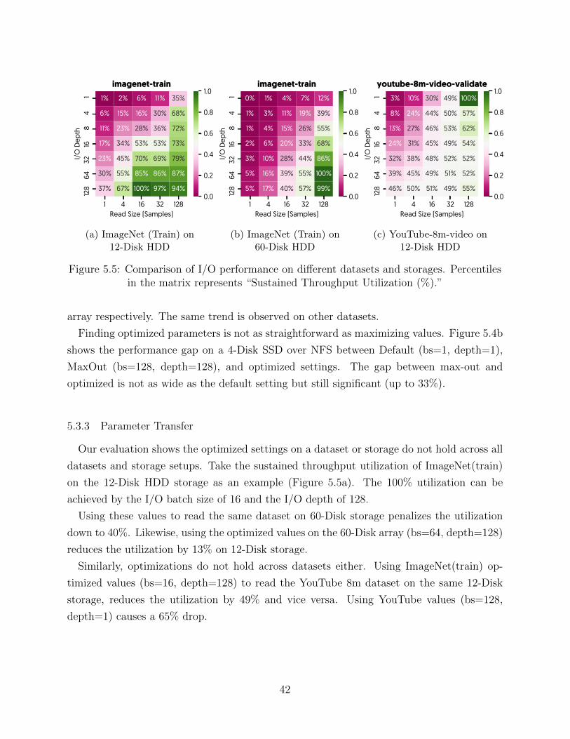
1 4 16 32 128Read Size (Samples)

14

816

3264

128

I/O

Dep

th

0% 1% 2% 3% 7%

1% 4% 14% 18% 19%

2% 7% 23% 28% 29%

3% 10% 35% 40% 52%

4% 15% 49% 54% 70%

6% 20% 64% 67% 87%

7% 25% 77% 80% 100%

AirFreight-all

1 4 16 32 128Read Size (Samples)

14

816

3264

128

I/O

Dep

th

1% 3% 9% 18% 52%

10% 20% 25% 43% 80%

17% 33% 32% 48% 84%

25% 48% 49% 59% 84%

36% 65% 64% 72% 86%

47% 82% 79% 85% 90%

57% 100% 91% 95% 100%

COCO-test

1 4 16 32 128Read Size (Samples)

14

816

3264

128

I/O

Dep

th

2% 5% 10% 18% 54%

10% 19% 26% 44% 84%

17% 32% 32% 51% 87%

26% 48% 51% 60% 87%

36% 65% 67% 74% 92%

47% 81% 82% 88% 95%

57% 97% 95% 97% 100%

COCO-train

1 4 16 32 128Read Size (Samples)

14

816

3264

128

I/O

Dep

th

2% 3% 9% 18% 52%

10% 21% 25% 44% 77%

17% 32% 31% 48% 82%

26% 48% 47% 59% 82%

36% 65% 62% 74% 84%

48% 82% 76% 88% 87%

58% 100% 88% 99% 91%

COCO-val

1 4 16 32 128Read Size (Samples)

14

816

3264

128

I/O

Dep

th

1% 2% 5% 10% 28%

5% 13% 13% 26% 60%

9% 21% 23% 33% 64%

13% 30% 43% 50% 71%

19% 40% 56% 68% 82%

25% 50% 69% 83% 93%

31% 61% 82% 95% 100%

berkeley_segmentation-test

1 4 16 32 128Read Size (Samples)

14

816

3264

128

I/O

Dep

th

0% 2% 3% 6% 21%

3% 10% 8% 16% 49%

6% 16% 15% 21% 55%

9% 24% 28% 32% 64%

13% 33% 37% 43% 77%

18% 43% 46% 52% 91%

22% 52% 53% 60% 100%

berkeley_segmentation-train

1 4 16 32 128Read Size (Samples)

14

816

3264

128

I/O

Dep

th

1% 3% 8% 16% 49%

10% 19% 23% 41% 79%

16% 30% 30% 45% 84%

25% 45% 50% 57% 84%

36% 60% 67% 72% 88%

47% 76% 80% 87% 93%

57% 91% 92% 96% 100%

flickr30k-all

1 4 16 32 128Read Size (Samples)

14

816

3264

128

I/O

Dep

th

1% 3% 8% 16% 46%

9% 18% 22% 39% 78%

16% 29% 28% 43% 83%

25% 43% 46% 55% 84%

35% 58% 62% 70% 87%

46% 73% 76% 84% 94%

56% 89% 88% 94% 100%

flickr8k-all

1 4 16 32 128Read Size (Samples)

14

816

3264

128

I/O

Dep

th

0% 1% 2% 3% 10%

2% 6% 15% 19% 25%

3% 10% 24% 32% 33%

4% 16% 35% 46% 53%

6% 23% 47% 61% 70%

9% 30% 60% 76% 87%

11% 37% 74% 91% 100%

google_house_number-test

1 4 16 32 128Read Size (Samples)

14

816

3264

128

I/O

Dep

th

0% 0% 2% 3% 6%

1% 4% 13% 19% 16%

2% 6% 21% 30% 27%

3% 10% 32% 43% 52%

4% 15% 45% 57% 69%

5% 19% 58% 73% 85%

7% 24% 71% 89% 100%

google_house_number-train

1 4 16 32 128Read Size (Samples)

14

816

3264

128

I/O

Dep

th

1% 2% 6% 11% 35%

6% 15% 16% 30% 68%

11% 23% 28% 36% 72%

17% 34% 53% 53% 73%

23% 45% 70% 69% 79%

30% 55% 85% 86% 87%

37% 67% 100% 97% 94%

imagenet-train

1 4 16 32 128Read Size (Samples)

14

816

3264

128

I/O

Dep

th

1% 3% 8% 15% 42%

9% 19% 21% 37% 75%

14% 30% 30% 41% 79%

22% 43% 53% 55% 81%

31% 57% 70% 72% 86%

41% 71% 86% 85% 91%

51% 85% 100% 96% 97%

imagenet-validation

1 4 16 32 128Read Size (Samples)

14

816

3264

128

I/O

Dep

th

3% 11% 30% 51% 100%

8% 25% 46% 52% 59%

14% 28% 48% 54% 65%

26% 33% 46% 52% 55%

34% 39% 49% 52% 54%

41% 46% 50% 52% 52%

47% 50% 39% 52% 52%

youtube-8m-video-test

1 4 16 32 128Read Size (Samples)

14

816

3264

128

I/O

Dep

th

7% 21% 54% 73% 100%

18% 33% 42% 42% 50%

20% 35% 43% 44% 51%

23% 35% 40% 42% 40%

30% 37% 41% 40% 45%

34% 39% 38% 39% 42%

38% 40% 38% 40% 43%

youtube-8m-video-train

1 4 16 32 128Read Size (Samples)

14

816

3264

128

I/O

Dep

th

3% 10% 30% 49% 100%

8% 24% 44% 50% 57%

13% 27% 46% 53% 62%

24% 31% 45% 49% 54%

32% 38% 48% 52% 52%

39% 45% 49% 51% 52%

46% 50% 51% 49% 55%

youtube-8m-video-validate

0.0

0.2

0.4

0.6

0.8

1.0

0.0

0.2

0.4

0.6

0.8

1.0

0.0

0.2

0.4

0.6

0.8

1.0

0.0

0.2

0.4

0.6

0.8

1.0

0.0

0.2

0.4

0.6

0.8

1.0

0.0

0.2

0.4

0.6

0.8

1.0

0.0

0.2

0.4

0.6

0.8

1.0

0.0

0.2

0.4

0.6

0.8

1.0

0.0

0.2

0.4

0.6

0.8

1.0

0.0

0.2

0.4

0.6

0.8

1.0

0.0

0.2

0.4

0.6

0.8

1.0

0.0

0.2

0.4

0.6

0.8

1.0

0.0

0.2

0.4

0.6

0.8

1.0

0.0

0.2

0.4

0.6

0.8

1.0

0.0

0.2

0.4

0.6

0.8

1.0

(a) ImageNet (Train) on12-Disk HDD

1 4 16 32 128Read Size (Samples)

14

816

3264

128

I/O

Dep

th

0% 0% 2% 3% 9%

0% 1% 4% 8% 27%

0% 1% 6% 11% 38%

1% 2% 8% 16% 51%

1% 4% 15% 27% 70%

2% 7% 25% 42% 95%

2% 8% 27% 45% 100%

AirFreight-all

1 4 16 32 128Read Size (Samples)

14

816

3264

128

I/O

Dep

th

0% 2% 6% 10% 15%

1% 4% 15% 23% 44%

2% 6% 21% 33% 63%

2% 9% 26% 42% 76%

5% 15% 34% 54% 96%

8% 22% 44% 67% 100%

8% 24% 45% 69% 99%

COCO-test

1 4 16 32 128Read Size (Samples)

14

816

3264

128

I/O

Dep

th

0% 2% 6% 9% 15%

1% 4% 15% 24% 41%

2% 6% 21% 34% 63%

2% 9% 26% 42% 77%

4% 14% 34% 53% 95%

8% 22% 43% 67% 100%

8% 24% 45% 69% 99%

COCO-train

1 4 16 32 128Read Size (Samples)

14

816

3264

128

I/O

Dep

th

1% 2% 6% 10% 15%

1% 5% 15% 25% 44%

2% 6% 22% 36% 63%

3% 9% 27% 45% 77%

5% 15% 35% 57% 96%

8% 23% 45% 72% 100%

9% 25% 46% 74% 99%

COCO-val

1 4 16 32 128Read Size (Samples)

14

816

3264

128

I/O

Dep

th

0% 1% 3% 6% 14%

1% 2% 8% 14% 34%

1% 3% 11% 20% 50%

1% 4% 15% 26% 62%

2% 8% 21% 35% 79%

4% 12% 29% 46% 97%

4% 13% 31% 47% 100%

berkeley_segmentation-test

1 4 16 32 128Read Size (Samples)

14

816

3264

128

I/O

Dep

th

0% 1% 2% 5% 13%

0% 2% 6% 11% 33%

1% 2% 9% 16% 47%

1% 4% 12% 20% 61%

2% 6% 17% 27% 78%

3% 10% 24% 35% 97%

4% 11% 25% 36% 100%

berkeley_segmentation-train

1 4 16 32 128Read Size (Samples)

14

816

3264

128

I/O

Dep

th

0% 2% 5% 7% 14%

1% 4% 13% 22% 42%

2% 6% 19% 31% 59%

2% 8% 24% 39% 75%

4% 13% 32% 51% 94%

7% 20% 41% 64% 100%

8% 21% 42% 65% 99%

flickr30k-all

1 4 16 32 128Read Size (Samples)

14

816

3264

128

I/O

Dep

th

0% 2% 5% 9% 14%

1% 4% 13% 22% 42%

1% 5% 18% 31% 60%

2% 8% 23% 38% 74%

4% 13% 31% 49% 92%

7% 19% 39% 62% 100%

8% 21% 40% 63% 99%

flickr8k-all

1 4 16 32 128Read Size (Samples)

14

816

3264

128

I/O

Dep

th

0% 1% 2% 3% 12%

0% 1% 5% 9% 32%

0% 2% 7% 13% 45%

1% 3% 10% 19% 57%

1% 5% 18% 31% 75%

2% 9% 29% 47% 96%

3% 10% 31% 50% 100%

google_house_number-test

1 4 16 32 128Read Size (Samples)

14

816

3264

128

I/O

Dep

th

0% 0% 2% 3% 11%

0% 1% 4% 8% 26%

0% 1% 6% 11% 37%

1% 2% 8% 15% 49%

1% 4% 15% 27% 70%

2% 7% 25% 44% 95%

2% 8% 27% 47% 100%

google_house_number-train

1 4 16 32 128Read Size (Samples)

14

816

3264

128

I/O

Dep

th

0% 1% 4% 7% 12%

1% 3% 11% 19% 39%

1% 4% 15% 26% 55%

2% 6% 20% 33% 68%

3% 10% 28% 44% 86%

5% 16% 39% 55% 100%

5% 17% 40% 57% 99%

imagenet-train

1 4 16 32 128Read Size (Samples)

14

816

3264

128

I/O

Dep

th

0% 1% 5% 8% 14%

1% 4% 12% 21% 41%

1% 5% 18% 30% 58%

2% 7% 23% 37% 72%

4% 12% 31% 48% 91%

6% 19% 41% 61% 100%

7% 21% 43% 62% 99%

imagenet-validation

1 4 16 32 128Read Size (Samples)

14

816

3264

128

I/O

Dep

th

3% 9% 13% 15% 36%

8% 22% 38% 47% 87%

11% 32% 57% 67% 99%

15% 39% 69% 80% 100%

21% 50% 86% 94% 99%

28% 62% 88% 93% 97%

29% 64% 87% 92% 93%

youtube-8m-video-test

1 4 16 32 128Read Size (Samples)

14

816

3264

128

I/O

Dep

th

7% 12% 23% 32% 44%

19% 34% 63% 77% 93%

27% 49% 80% 87% 99%

33% 60% 80% 88% 100%

42% 75% 80% 87% 98%

52% 80% 79% 85% 97%

54% 78% 78% 82% 85%

youtube-8m-video-train

1 4 16 32 128Read Size (Samples)

14

816

3264

128

I/O

Dep

th

3% 9% 14% 15% 37%

8% 22% 40% 48% 89%

11% 31% 57% 67% 100%

15% 39% 70% 80% 100%

20% 50% 86% 95% 100%

28% 62% 88% 93% 97%

29% 63% 88% 93% 93%

youtube-8m-video-validate

0.0

0.2

0.4

0.6

0.8

1.0

0.0

0.2

0.4

0.6

0.8

1.0

0.0

0.2

0.4

0.6

0.8

1.0

0.0

0.2

0.4

0.6

0.8

1.0

0.0

0.2

0.4

0.6

0.8

1.0

0.0

0.2

0.4

0.6

0.8

1.0

0.0

0.2

0.4

0.6

0.8

1.0

0.0

0.2

0.4

0.6

0.8

1.0

0.0

0.2

0.4

0.6

0.8

1.0

0.0

0.2

0.4

0.6

0.8

1.0

0.0

0.2

0.4

0.6

0.8

1.0

0.0

0.2

0.4

0.6

0.8

1.0

0.0

0.2

0.4

0.6

0.8

1.0

0.0

0.2

0.4

0.6

0.8

1.0

0.0

0.2

0.4

0.6

0.8

1.0

(b) ImageNet (Train) on60-Disk HDD

1 4 16 32 128Read Size (Samples)

14

816

3264

128

I/O

Dep

th

0% 1% 2% 3% 7%

1% 4% 14% 18% 19%

2% 7% 23% 28% 29%

3% 10% 35% 40% 52%

4% 15% 49% 54% 70%

6% 20% 64% 67% 87%

7% 25% 77% 80% 100%

AirFreight-all

1 4 16 32 128Read Size (Samples)

14

816

3264

128

I/O

Dep

th

1% 3% 9% 18% 52%

10% 20% 25% 43% 80%

17% 33% 32% 48% 84%

25% 48% 49% 59% 84%

36% 65% 64% 72% 86%

47% 82% 79% 85% 90%

57% 100% 91% 95% 100%

COCO-test

1 4 16 32 128Read Size (Samples)

14

816

3264

128

I/O

Dep

th

2% 5% 10% 18% 54%

10% 19% 26% 44% 84%

17% 32% 32% 51% 87%

26% 48% 51% 60% 87%

36% 65% 67% 74% 92%

47% 81% 82% 88% 95%

57% 97% 95% 97% 100%

COCO-train

1 4 16 32 128Read Size (Samples)

14

816

3264

128

I/O

Dep

th

2% 3% 9% 18% 52%

10% 21% 25% 44% 77%

17% 32% 31% 48% 82%

26% 48% 47% 59% 82%

36% 65% 62% 74% 84%

48% 82% 76% 88% 87%

58% 100% 88% 99% 91%

COCO-val

1 4 16 32 128Read Size (Samples)

14

816

3264

128

I/O

Dep

th

1% 2% 5% 10% 28%

5% 13% 13% 26% 60%

9% 21% 23% 33% 64%

13% 30% 43% 50% 71%

19% 40% 56% 68% 82%

25% 50% 69% 83% 93%

31% 61% 82% 95% 100%

berkeley_segmentation-test

1 4 16 32 128Read Size (Samples)

14

816

3264

128

I/O

Dep

th

0% 2% 3% 6% 21%

3% 10% 8% 16% 49%

6% 16% 15% 21% 55%

9% 24% 28% 32% 64%

13% 33% 37% 43% 77%

18% 43% 46% 52% 91%

22% 52% 53% 60% 100%

berkeley_segmentation-train

1 4 16 32 128Read Size (Samples)

14

816

3264

128

I/O

Dep

th

1% 3% 8% 16% 49%

10% 19% 23% 41% 79%

16% 30% 30% 45% 84%

25% 45% 50% 57% 84%

36% 60% 67% 72% 88%

47% 76% 80% 87% 93%

57% 91% 92% 96% 100%

flickr30k-all

1 4 16 32 128Read Size (Samples)

14

816

3264

128

I/O

Dep

th

1% 3% 8% 16% 46%

9% 18% 22% 39% 78%

16% 29% 28% 43% 83%

25% 43% 46% 55% 84%

35% 58% 62% 70% 87%

46% 73% 76% 84% 94%

56% 89% 88% 94% 100%

flickr8k-all

1 4 16 32 128Read Size (Samples)

14

816

3264

128

I/O

Dep

th

0% 1% 2% 3% 10%

2% 6% 15% 19% 25%

3% 10% 24% 32% 33%

4% 16% 35% 46% 53%

6% 23% 47% 61% 70%

9% 30% 60% 76% 87%

11% 37% 74% 91% 100%

google_house_number-test

1 4 16 32 128Read Size (Samples)

14

816

3264

128

I/O

Dep

th

0% 0% 2% 3% 6%

1% 4% 13% 19% 16%

2% 6% 21% 30% 27%

3% 10% 32% 43% 52%

4% 15% 45% 57% 69%

5% 19% 58% 73% 85%

7% 24% 71% 89% 100%

google_house_number-train

1 4 16 32 128Read Size (Samples)

14

816

3264

128

I/O

Dep

th

1% 2% 6% 11% 35%

6% 15% 16% 30% 68%

11% 23% 28% 36% 72%

17% 34% 53% 53% 73%

23% 45% 70% 69% 79%

30% 55% 85% 86% 87%

37% 67% 100% 97% 94%

imagenet-train

1 4 16 32 128Read Size (Samples)

14

816

3264

128

I/O

Dep

th

1% 3% 8% 15% 42%

9% 19% 21% 37% 75%

14% 30% 30% 41% 79%

22% 43% 53% 55% 81%

31% 57% 70% 72% 86%

41% 71% 86% 85% 91%

51% 85% 100% 96% 97%

imagenet-validation

1 4 16 32 128Read Size (Samples)

14

816

3264

128

I/O

Dep

th

3% 11% 30% 51% 100%

8% 25% 46% 52% 59%

14% 28% 48% 54% 65%

26% 33% 46% 52% 55%

34% 39% 49% 52% 54%

41% 46% 50% 52% 52%

47% 50% 39% 52% 52%

youtube-8m-video-test

1 4 16 32 128Read Size (Samples)

14

816

3264

128

I/O

Dep

th

7% 21% 54% 73% 100%

18% 33% 42% 42% 50%

20% 35% 43% 44% 51%

23% 35% 40% 42% 40%

30% 37% 41% 40% 45%

34% 39% 38% 39% 42%

38% 40% 38% 40% 43%

youtube-8m-video-train

1 4 16 32 128Read Size (Samples)

14

816

3264

128

I/O

Dep

th

3% 10% 30% 49% 100%

8% 24% 44% 50% 57%

13% 27% 46% 53% 62%

24% 31% 45% 49% 54%

32% 38% 48% 52% 52%

39% 45% 49% 51% 52%

46% 50% 51% 49% 55%

youtube-8m-video-validate

0.0

0.2

0.4

0.6

0.8

1.0

0.0

0.2

0.4

0.6

0.8

1.0

0.0

0.2

0.4

0.6

0.8

1.0

0.0

0.2

0.4

0.6

0.8

1.0

0.0

0.2

0.4

0.6

0.8

1.0

0.0

0.2

0.4

0.6

0.8

1.0

0.0

0.2

0.4

0.6

0.8

1.0

0.0

0.2

0.4

0.6

0.8

1.0

0.0

0.2

0.4

0.6

0.8

1.0

0.0

0.2

0.4

0.6

0.8

1.0

0.0

0.2

0.4

0.6

0.8

1.0

0.0

0.2

0.4

0.6

0.8

1.0

0.0

0.2

0.4

0.6

0.8

1.0

0.0

0.2

0.4

0.6

0.8

1.0

0.0

0.2

0.4

0.6

0.8

1.0

(c) YouTube-8m-video on12-Disk HDD

Figure 5.5: Comparison of I/O performance on different datasets and storages. Percentilesin the matrix represents “Sustained Throughput Utilization (%).”

array respectively. The same trend is observed on other datasets.

Finding optimized parameters is not as straightforward as maximizing values. Figure 5.4b

shows the performance gap on a 4-Disk SSD over NFS between Default (bs=1, depth=1),

MaxOut (bs=128, depth=128), and optimized settings. The gap between max-out and

optimized is not as wide as the default setting but still significant (up to 33%).

5.3.3 Parameter Transfer

Our evaluation shows the optimized settings on a dataset or storage do not hold across all

datasets and storage setups. Take the sustained throughput utilization of ImageNet(train)

on the 12-Disk HDD storage as an example (Figure 5.5a). The 100% utilization can be

achieved by the I/O batch size of 16 and the I/O depth of 128.

Using these values to read the same dataset on 60-Disk storage penalizes the utilization

down to 40%. Likewise, using the optimized values on the 60-Disk array (bs=64, depth=128)

reduces the utilization by 13% on 12-Disk storage.

Similarly, optimizations do not hold across datasets either. Using ImageNet(train) op-

timized values (bs=16, depth=128) to read the YouTube 8m dataset on the same 12-Disk

storage, reduces the utilization by 49% and vice versa. Using YouTube values (bs=128,

depth=1) causes a 65% drop.

42

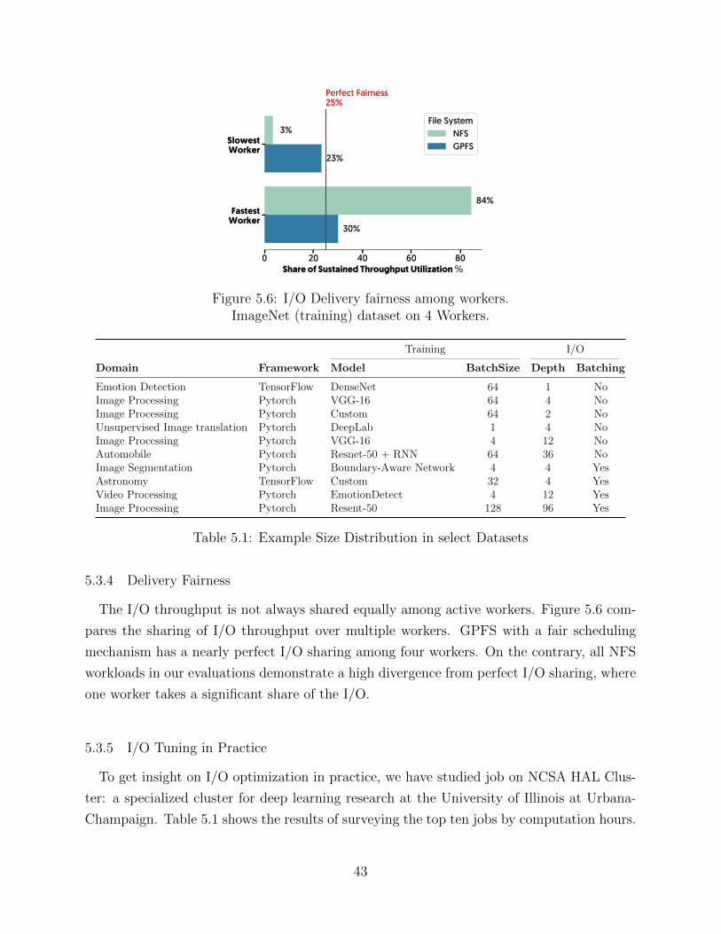
0 20 40 60 80Share of Sustained Throughput Utilization %

SlowestWorker

FastestWorker

Perfect Fairness25%

3%

84%

23%

30%

File SystemNFSGPFS

Figure 5.6: I/O Delivery fairness among workers.ImageNet (training) dataset on 4 Workers.

Training I/O

Domain Framework Model BatchSize Depth Batching

Emotion Detection TensorFlow DenseNet 64 1 NoImage Processing Pytorch VGG-16 64 4 NoImage Processing Pytorch Custom 64 2 NoUnsupervised Image translation Pytorch DeepLab 1 4 NoImage Processing Pytorch VGG-16 4 12 NoAutomobile Pytorch Resnet-50 + RNN 64 36 NoImage Segmentation Pytorch Boundary-Aware Network 4 4 YesAstronomy TensorFlow Custom 32 4 YesVideo Processing Pytorch EmotionDetect 4 12 YesImage Processing Pytorch Resent-50 128 96 Yes

Table 5.1: Example Size Distribution in select Datasets

5.3.4 Delivery Fairness

The I/O throughput is not always shared equally among active workers. Figure 5.6 com-

pares the sharing of I/O throughput over multiple workers. GPFS with a fair scheduling

mechanism has a nearly perfect I/O sharing among four workers. On the contrary, all NFS

workloads in our evaluations demonstrate a high divergence from perfect I/O sharing, where

one worker takes a significant share of the I/O.

5.3.5 I/O Tuning in Practice

To get insight on I/O optimization in practice, we have studied job on NCSA HAL Clus-

ter: a specialized cluster for deep learning research at the University of Illinois at Urbana-

Champaign. Table 5.1 shows the results of surveying the top ten jobs by computation hours.

43

Out of 10 jobs, six do not use I/O batching at all, and six use a small I/O depth (¡=4). Only

in 2 jobs, both I/O batch and depth are set significantly beyond the default behavior.

5.4 CONCLUSION

In this chapter, we show that I/O tuning has a huge impact on the I/O throughput,

which could be as wide as three orders of magnitude improvement on throughput. Optimized

settings do not hold across all datasets and storages, and simply maximizing I/O parameters

does not usually lead to optimal throughput. Lastly, our user survey shows that users in

practice are not properly tuning the I/O.

We propose Diot to automate the I/O tuning for modern ML workloads by accelerating

the parameter grid search. Diot improves the I/O throughput up to 3 orders of magnitude

compared to default I/O settings.

44

CHAPTER 6: COMMUNICATION SCHEDULING OF CAUSALDEPENDENCIES

State-of-the-art deep learning systems rely on iterative distributed training to tackle the

increasing complexity of models and input data. In this work, we identify an opportunity for

accelerating distributed DNN training in systems that rely on graph representation for com-

putation, such as TensorFlow and PyTorch, through communication scheduling. We develop

a system, TicTac, that reduces the iteration time by identifying and enforcing parameter

transfers in the order in which the parameters are consumed by the underlying computational

model, thereby guaranteeing near-optimal overlap of communication and computation. Our

system is implemented over TensorFlow and enforces the optimal ordering by prioritization

of parameter transfers at the Parameter Server in data parallel training. TicTac requires

no changes to the model or developer inputs and improves the throughput by up to 37.7%

in inference and 19.2% in training, while also reducing straggler effect by up to 2.3×. Our

code is publicly available.

6.1 INTRODUCTION

Deep learning has grown significantly in the past decade, fuelled by the flexibility of de-

velopment offered by machine learning frameworks, availability of rich data, and readily

accessible distributed high-performance computing. The computational cost of training so-

phisticated deep learning models has long outgrown the capabilities of a single high-end

machine, leading to distributed training being the norm in a typical AI pipeline. Training

a deep learning model is an iterative job which may take days to weeks in high-end clusters

today.

Computational graphs are used to represent the training jobs in state-of-the-art systems [1,

21, 80]. In the commonly-used Model Replica or data parallel mode of training, the input

data is partitioned and processed at participating workers using identical computational

graphs. Each iteration typically lasts milliseconds to seconds. At the end of each iteration,

servers exchange a relatively large amount of data associated with parameter updates to

aggregate the results of the iteration. This communication overhead has a substantial impact

on throughput of the system and also limits its scalability [96, 5]. Even a small improvement

in communication overhead can improve the learning time by hours in these long-running

learning jobs.

The iteration time in deep learning systems depends on the time taken by (i) computation,

(ii) communication and (iii) the overlap between the two. When workers receive the param-

45

eters from the parameter server at the beginning of each iteration, all parameters are not

used simultaneously; they are consumed based on the dependencies in the underlying DAG.

While one particular schedule of parameter transfers (over the complete set of parameters

in a given model in a single iteration) may facilitate faster computation, another may cause

blockage. Hence, identifying the best schedule of parameter transfers is critical for reducing

the blocking on computation (determined by DAG dependencies), and in turn improving

the overlap and the iteration time.

We observe that the schedule of data transfers in current systems [1, 21, 80] is deter-

mined arbitrarily during execution without considering the impact on overlap. We quantify

the observed combinations in TensorFlow and find that in a trial with 1000 iterations on

ResNet-V2-50, every iteration had a unique order of received parameters which has not been

observed previously. This random order of parameter transfers at workers has two perfor-

mance implications. First, the iteration time, and in turn throughput (number of samples

processed per second), suffers significantly due to sub-optimal overlap. Second, even in the

same iteration, multiple workers might follow different schedules of data transfers, leading

to stragglers during synchronized training.

Past work has attempted to address this issue by enforcing the same order of parameter

transfers at all workers. However, these solutions are restricted to earlier systems with

layer-by-layer model representation [8, 29, 116] where finding the optimal order of execution

is trivial [28]. In modern systems with DAG representation [1, 80], this is a non-trivial

challenge.

In this work, we devise a systematic methodology for deriving near-optimal schedules of

parameter transfers through critical path analysis on the underlying computational graph.

This allows maximal overlap of computation and communication and prevents stragglers

arising from random order of parameter transfers at workers. We also develop a lightweight

resource-level enforcement mechanism over TensorFlow [1]. These techniques form the core

of our system, TicTac, which achieves substantial performance improvement while requiring

no changes in the model or developer inputs.

In summary, we make the following contributions:

• We identify an opportunity for improving performance in state-of-the-art deep learning

systems with Parameter Server-based aggregation through prioritized parameter transfers

(§6.2).

• We define a metric to quantify the efficiency of a given execution: the overlap coefficient

(§6.3).

• We propose two heuristics, TIC and TAC, for near-optimal scheduling of computation and

46

communication in Model Replica with Parameter Server.

• We implement our system over TensorFlow (§ 6.5). The code is publicly available1.

• We extensively evaluate the performance of our system in GPU and high-end CPU envi-

ronments under training and inference of DNN models and show that throughput can be

improved by up to 37% (§6.6).

6.2 BACKGROUND AND MOTIVATION

Our system focuses on network optimization in deep learning frameworks with DAG rep-

resentation of computational graphs [1, 80], Model Replica (MR) mode of distribution and

Parameter Servers. The performance improvement provided by TicTac is beneficial in two

key environments. First, it improves throughput and iteration time in clud environment

with commodity hardware or on-demand clusters where high resiliency is critical (workers

may be preempted). Second, in online reinforcement learning with workers for training and

separate active agents for inference, enforced ordering can improve the inference time. In this

environment, the active agents are reading parameters from the PS or decentralized workers

as shown in Figure 6.3. While decentralized aggregation techniques (such as all-reduce and

Horovod [90]) are gaining traction in high performance networking, TicTac does not address

such systems and is focused on PS.

In this section, we give a brief overview of deep learning systems, prior techniques proposed

in these systems to mitigate network overhead, and opportunities for further optimization.

6.2.1 Network Optimization in DNN training

In deep learning systems, high GPU utilization can be achieved in two ways: (i) when

total communication time is less than or equal to the computation time and (ii) with effi-

cient overlap of communication and computation. Several techniques have been proposed to

improve GPU utilization.

Increasing computation time: The fraction of computation time relative to commu-

nication time can be increased by increasing the batch size [52]. However, this approach

suffers from decreased accuracy [60] and may not be generally applicable under resource

constraints. [37, 25, 113, 4].

Decreasing communication time: Solutions for reducing network communication have

1https://github.com/xldrx/tictac

47

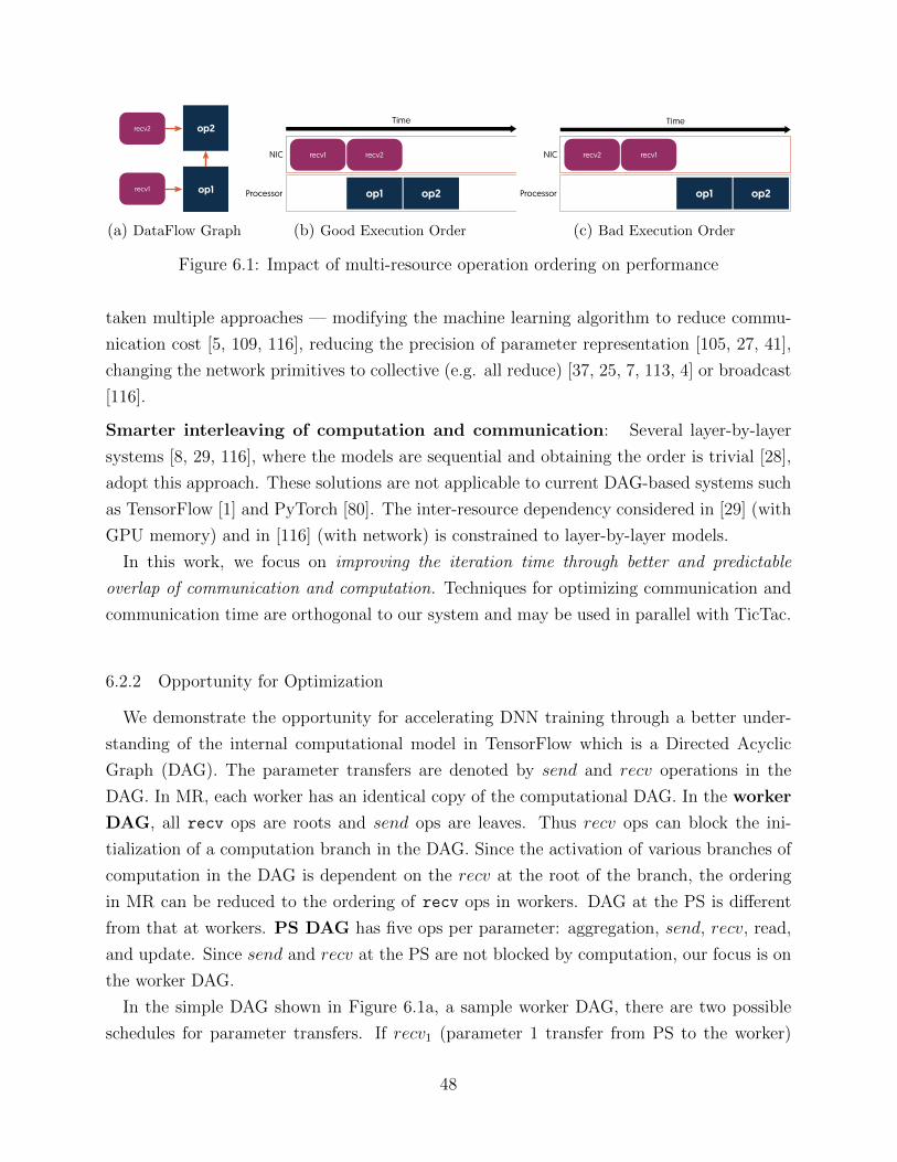
op2

op1recv1

recv2

(a) DataFlow Graph

op2op1

recv2recv1NIC

Processor

Time

(b) Good Execution Order

op2op1

recv1recv2NIC

Processor

Time

(c) Bad Execution Order

Figure 6.1: Impact of multi-resource operation ordering on performance

taken multiple approaches — modifying the machine learning algorithm to reduce commu-

nication cost [5, 109, 116], reducing the precision of parameter representation [105, 27, 41],

changing the network primitives to collective (e.g. all reduce) [37, 25, 7, 113, 4] or broadcast

[116].

Smarter interleaving of computation and communication: Several layer-by-layer

systems [8, 29, 116], where the models are sequential and obtaining the order is trivial [28],

adopt this approach. These solutions are not applicable to current DAG-based systems such

as TensorFlow [1] and PyTorch [80]. The inter-resource dependency considered in [29] (with

GPU memory) and in [116] (with network) is constrained to layer-by-layer models.

In this work, we focus on improving the iteration time through better and predictable

overlap of communication and computation. Techniques for optimizing communication and

communication time are orthogonal to our system and may be used in parallel with TicTac.

6.2.2 Opportunity for Optimization

We demonstrate the opportunity for accelerating DNN training through a better under-

standing of the internal computational model in TensorFlow which is a Directed Acyclic

Graph (DAG). The parameter transfers are denoted by send and recv operations in the

DAG. In MR, each worker has an identical copy of the computational DAG. In the worker

DAG, all recv ops are roots and send ops are leaves. Thus recv ops can block the ini-

tialization of a computation branch in the DAG. Since the activation of various branches of

computation in the DAG is dependent on the recv at the root of the branch, the ordering

in MR can be reduced to the ordering of recv ops in workers. DAG at the PS is different

from that at workers. PS DAG has five ops per parameter: aggregation, send, recv, read,

and update. Since send and recv at the PS are not blocked by computation, our focus is on

the worker DAG.

In the simple DAG shown in Figure 6.1a, a sample worker DAG, there are two possible

schedules for parameter transfers. If recv1 (parameter 1 transfer from PS to the worker)

48

happens before recv2 (parameter 2 transfer), it reduces the blocking on computation time and

improves the overlap. The reverse order results in increased iteration time due to blocking

on computation. Thus, in a distributed environment, network can block computation based

on dependencies in the DAG. This can lead to under-utilization of computational capacity,

in turn resulting in sub-optimal performance. In addition, variation in iteration time caused

by random order of parameter transfers across multiple workers can lead to straggling effect.

The impact of poor overlap can be significant in DNN training due to complexity of state-

of-the-art models. For instance, ResNet-v2-152 [50] has 363 parameters with an aggregate

size of 229.5MB. The computational graph associated with this neural network has 4655

operations in the TensorFlow framework. Finding the optimal schedule in this complex DAG

involves evaluating 363! combinations. We run 1000 iterations of learning over ResNet-v2-

50, Inception-v3 and VGG-16 networks and observe the order of network transfers at a single

worker. The observed order of parameter transfer is unique in ResNet-v2-50 and Inception-

v3 networks across the 1000 runs. In VGG-16, we observe 493 unique combinations across

1000 runs.

6.2.3 Comparison with Other Distributed Systems

It is worth noting that deep learning systems with computational graphs are fundamentally

different from graph processing systems [70, 51, 110]. In deep learning, the graph is a

representation of the computation to be done on the input data. In graph processing systems,

the graph itself is the input to the computation. As a result, graphs in DNN frameworks

are a few orders of magnitude smaller than a typical large-scale graph processing system.

Iterations in DNN frameworks are identical, and network communication pattern is fixed.

This may not be true for graph processing systems.

In stream processing systems, the relationship between processing elements are represented

using graphs. These systems allow pipelining, with different partitions of input data being

processed in different elements along the pipeline at the same time. In contrast, DNN

frameworks process the entire batch of input at a processing element at a worker. Pipelining

is not employed in this environment. Hence, optimizations proposed for stream processing

cannot be borrowed here.

6.3 QUANTIFYING PERFORMANCE

In this section, we explore methods for quantitatively comparing the efficiency of multiple

schedules. Towards this goal, we formally define the scheduling problem and investigate the

49

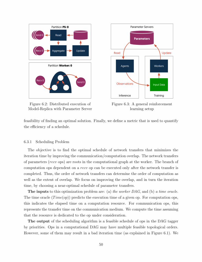
Partition Worker: 0

Partition PS: 0

Aggregate

Recv 0Send 0

Recv 0

Send 0

Update

Read

Figure 6.2: Distributed execution ofModel-Replica with Parameter Server

Parameter Servers

Inference

Parameters

Agents

Training

Workers

Input Data

Read Update

Observations

Figure 6.3: A general reinforcementlearning setup

feasibility of finding an optimal solution. Finally, we define a metric that is used to quantify

the efficiency of a schedule.

6.3.1 Scheduling Problem

The objective is to find the optimal schedule of network transfers that minimizes the

iteration time by improving the communication/computation overlap. The network transfers

of parameters (recv ops) are roots in the computational graph at the worker. The branch of

computation ops dependent on a recv op can be executed only after the network transfer is

completed. Thus, the order of network transfers can determine the order of computation as

well as the extent of overlap. We focus on improving the overlap, and in turn the iteration

time, by choosing a near-optimal schedule of parameter transfers.

The inputs to this optimization problem are: (a) the worker DAG, and (b) a time oracle.

The time oracle (Time(op)) predicts the execution time of a given op. For computation ops,

this indicates the elapsed time on a computation resource. For communication ops, this

represents the transfer time on the communication medium. We compute the time assuming

that the resource is dedicated to the op under consideration.

The output of the scheduling algorithm is a feasible schedule of ops in the DAG tagger

by priorities. Ops in a computational DAG may have multiple feasible topological orders.

However, some of them may result in a bad iteration time (as explained in Figure 6.1). We

50

want to limit the execution path to take the one that improves the training performance.

We achieve this with priority numbers. Priority number is a positive integer assigned to an

op in the DAG. A higher priority op is given a lower priority number. An op may not be

assigned a priority if it need not be ordered. Multiple ops may be assigned the same priority

if their relative order is insignificant.

The order is enforced in the following manner. When we need to select a new op from

the ready-to-execute queue, we randomly choose from among the set of ops that contain

the lowest priority number and those without any priority number. It is worth noting that

priority only specifies relative order among candidate ops in the ready-to-execute queue at

a given resource, and the resulting order will still respect the topological order specified by

the DAG.

The problem of finding the optimal schedule is NP-hard. A simpler version of the optimal

execution problem with homogeneous hardware can be formally defined as follow (Using

notation in [83]): Pm|Mi, prec|CmaxIn this formulation, Pm represents multiple parallel resources with identical performance.

Mi assigns the operations to specific resources, i.e., computation ops vs. communication.

prec describes the dependency relation of ops in the DAG. The Cmax represents the goal of

scheduling is to minimize the last node completion time.

This problem is still open [19] and simpler cases are proven to be NP-Hard. While there

exist approximations for relaxed versions of this problem, to the best of our knowledge, there

is no solution or approximation with guaranteed bounds for our original problem.

6.3.2 Defining Overlap Coefficient

The two major contributors to total DNN iteration time (T ) are network transfer time

or the communication time (N) and the computation time (C). Since the computation

and communication may overlap, the total time T ≤ N + C. Given a GPU/CPU/TPU

environment, we assume the computation time, C, to be constant. We ignore the case of

computation stragglers and focus on communication.

We define two metrics that define the DNN iteration time: (a) the communication/compu-

tation ratio, ρ and (b) the overlap coefficient, α. The ratio of communication to computation,

denoted by ρ, determines the extent of benefits achievable. When ρ < 1, communication

time is smaller than the total computation time, providing ample opportunity for running

GPUs at high utilization.

The second factor affecting the GPU utilization is the overlap coefficient, α = N+C−Tmin(N ,C)

.

N +C is the iteration time when there is no overlap, and T is the actual iteration time. The

51

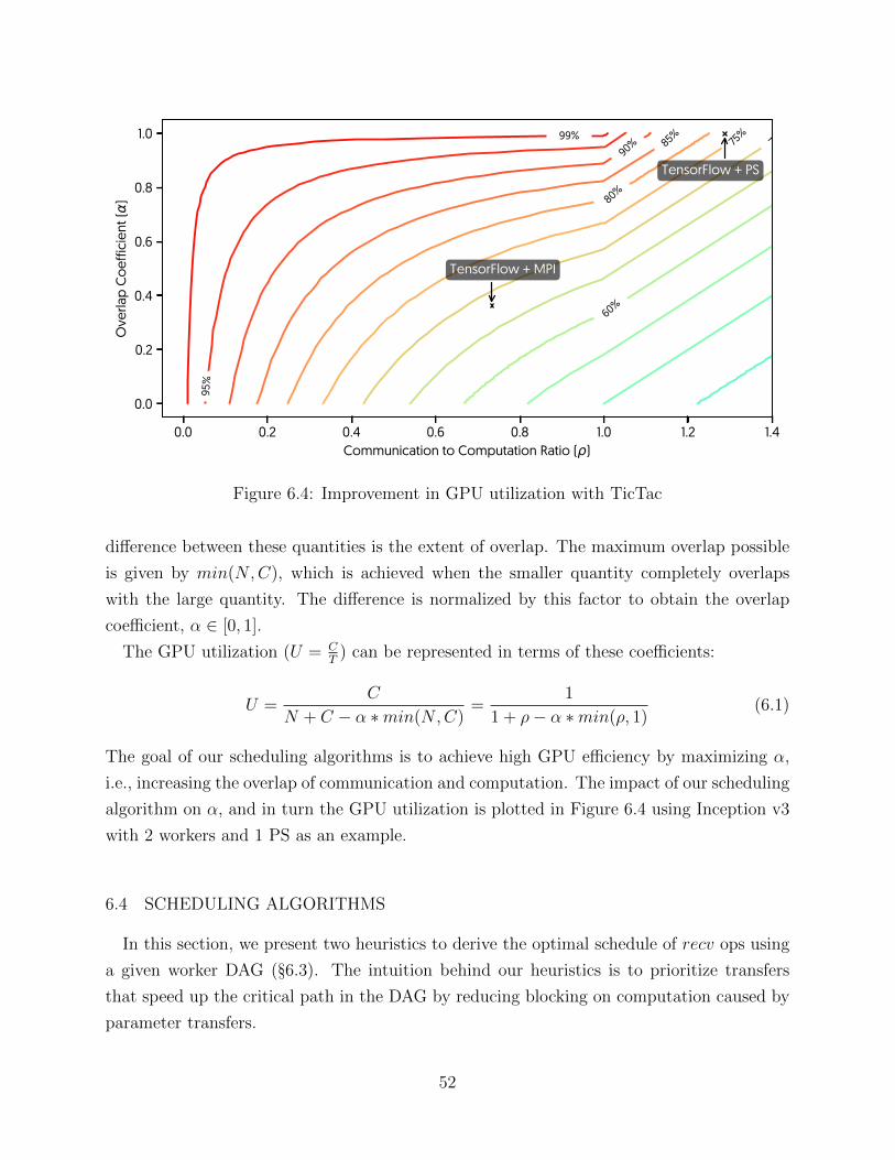
0.0 0.2 0.4 0.6 0.8 1.0 1.2 1.4Communication to Computation Ratio ( )

0.0

0.2

0.4

0.6

0.8

1.0O

verla

p C

oeffi

cien

t ()

TensorFlow + MPI

TensorFlow + PS

35%

40%

45%

50%

55%

60%

65%70%

75%

80%

85%

90%

95%

99%

Figure 6.4: Improvement in GPU utilization with TicTac

difference between these quantities is the extent of overlap. The maximum overlap possible

is given by min(N ,C), which is achieved when the smaller quantity completely overlaps

with the large quantity. The difference is normalized by this factor to obtain the overlap

coefficient, α ∈ [0, 1].

The GPU utilization (U = CT

) can be represented in terms of these coefficients:

U =C

N + C − α ∗min(N ,C)=

1

1 + ρ− α ∗min(ρ, 1)(6.1)

The goal of our scheduling algorithms is to achieve high GPU efficiency by maximizing α,

i.e., increasing the overlap of communication and computation. The impact of our scheduling

algorithm on α, and in turn the GPU utilization is plotted in Figure 6.4 using Inception v3

with 2 workers and 1 PS as an example.

6.4 SCHEDULING ALGORITHMS

In this section, we present two heuristics to derive the optimal schedule of recv ops using

a given worker DAG (§6.3). The intuition behind our heuristics is to prioritize transfers

that speed up the critical path in the DAG by reducing blocking on computation caused by

parameter transfers.

52

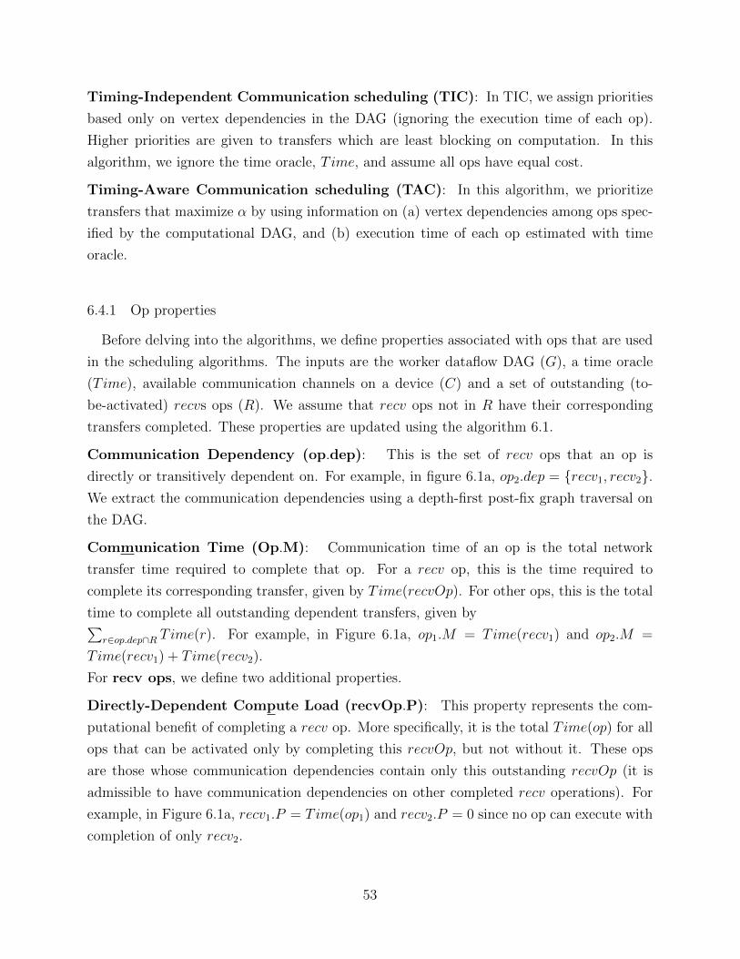
Timing-Independent Communication scheduling (TIC): In TIC, we assign priorities

based only on vertex dependencies in the DAG (ignoring the execution time of each op).

Higher priorities are given to transfers which are least blocking on computation. In this

algorithm, we ignore the time oracle, Time, and assume all ops have equal cost.

Timing-Aware Communication scheduling (TAC): In this algorithm, we prioritize

transfers that maximize α by using information on (a) vertex dependencies among ops spec-

ified by the computational DAG, and (b) execution time of each op estimated with time

oracle.

6.4.1 Op properties

Before delving into the algorithms, we define properties associated with ops that are used

in the scheduling algorithms. The inputs are the worker dataflow DAG (G), a time oracle

(Time), available communication channels on a device (C) and a set of outstanding (to-

be-activated) recvs ops (R). We assume that recv ops not in R have their corresponding

transfers completed. These properties are updated using the algorithm 6.1.

Communication Dependency (op.dep): This is the set of recv ops that an op is

directly or transitively dependent on. For example, in figure 6.1a, op2.dep = {recv1, recv2}.We extract the communication dependencies using a depth-first post-fix graph traversal on

the DAG.

Communication Time (Op.M): Communication time of an op is the total network

transfer time required to complete that op. For a recv op, this is the time required to

complete its corresponding transfer, given by Time(recvOp). For other ops, this is the total

time to complete all outstanding dependent transfers, given by∑r∈op.dep∩R Time(r). For example, in Figure 6.1a, op1.M = Time(recv1) and op2.M =

Time(recv1) + Time(recv2).

For recv ops, we define two additional properties.

Directly-Dependent Compute Load (recvOp.P): This property represents the com-

putational benefit of completing a recv op. More specifically, it is the total Time(op) for all

ops that can be activated only by completing this recvOp, but not without it. These ops

are those whose communication dependencies contain only this outstanding recvOp (it is

admissible to have communication dependencies on other completed recv operations). For

example, in Figure 6.1a, recv1.P = Time(op1) and recv2.P = 0 since no op can execute with

completion of only recv2.

53

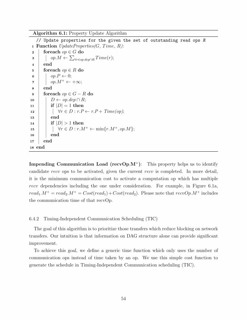
Algorithm 6.1: Property Update Algorithm

// Update properties for the given the set of outstanding read ops R

1 Function UpdateProperties(G, Time, R):2 foreach op ∈ G do3 op.M ←

∑∀r∈op.dep∩R Time(r);

4 end5 foreach op ∈ R do6 op.P ← 0;7 op.M+ ← +∞;

8 end9 foreach op ∈ G−R do

10 D ← op.dep ∩R;11 if |D| = 1 then12 ∀r ∈ D : r.P← r.P + Time(op);13 end14 if |D| > 1 then15 ∀r ∈ D : r.M+ ← min{r.M+, op.M};16 end

17 end

18 end

Impending Communication Load (recvOp.M+): This property helps us to identify

candidate recv ops to be activated, given the current recv is completed. In more detail,

it is the minimum communication cost to activate a computation op which has multiple

recv dependencies including the one under consideration. For example, in Figure 6.1a,

read1.M+ = read2.M

+ = Cost(read1)+Cost(read2). Please note that recvOp.M+ includes

the communication time of that recvOp.

6.4.2 Timing-Independent Communication Scheduling (TIC)

The goal of this algorithm is to prioritize those transfers which reduce blocking on network

transfers. Our intuition is that information on DAG structure alone can provide significant

improvement.

To achieve this goal, we define a generic time function which only uses the number of

communication ops instead of time taken by an op. We use this simple cost function to

generate the schedule in Timing-Independent Communication scheduling (TIC).

54

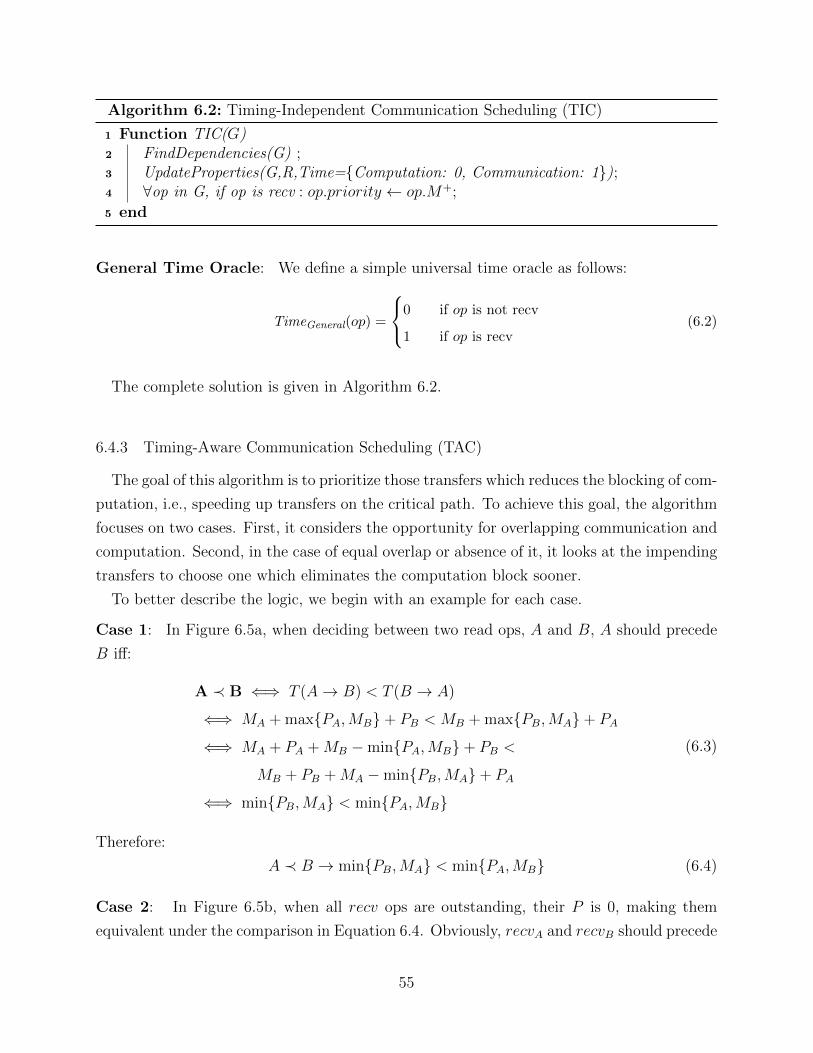
Algorithm 6.2: Timing-Independent Communication Scheduling (TIC)

1 Function TIC(G)2 FindDependencies(G) ;3 UpdateProperties(G,R,Time={Computation: 0, Communication: 1});4 ∀op in G, if op is recv : op.priority ← op.M+;

5 end

General Time Oracle: We define a simple universal time oracle as follows:

TimeGeneral(op) =

0 if op is not recv

1 if op is recv(6.2)

The complete solution is given in Algorithm 6.2.

6.4.3 Timing-Aware Communication Scheduling (TAC)

The goal of this algorithm is to prioritize those transfers which reduces the blocking of com-

putation, i.e., speeding up transfers on the critical path. To achieve this goal, the algorithm

focuses on two cases. First, it considers the opportunity for overlapping communication and

computation. Second, in the case of equal overlap or absence of it, it looks at the impending

transfers to choose one which eliminates the computation block sooner.

To better describe the logic, we begin with an example for each case.

Case 1: In Figure 6.5a, when deciding between two read ops, A and B, A should precede

B iff:

A ≺ B ⇐⇒ T (A→ B) < T (B → A)

⇐⇒ MA + max{PA,MB}+ PB < MB + max{PB,MA}+ PA

⇐⇒ MA + PA +MB −min{PA,MB}+ PB <

MB + PB +MA −min{PB,MA}+ PA

⇐⇒ min{PB,MA} < min{PA,MB}

(6.3)

Therefore:

A ≺ B → min{PB,MA} < min{PA,MB} (6.4)

Case 2: In Figure 6.5b, when all recv ops are outstanding, their P is 0, making them

equivalent under the comparison in Equation 6.4. Obviously, recvA and recvB should precede

55

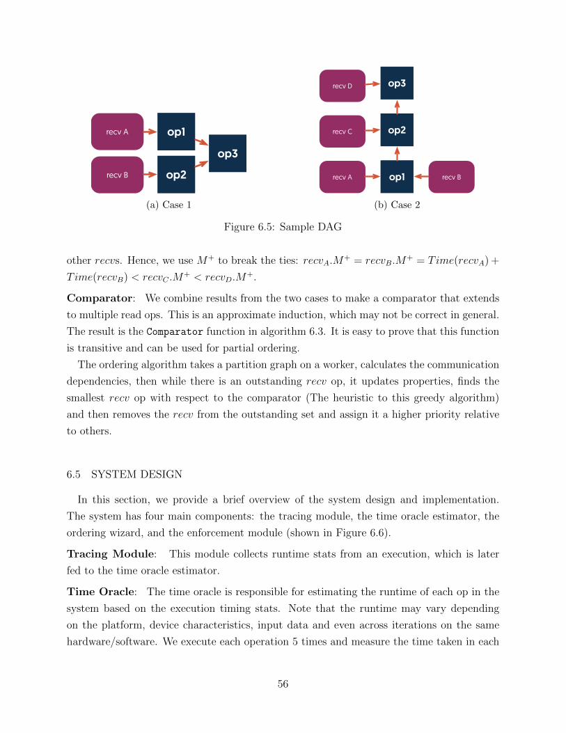
op3

op1recv A

recv B op2

(a) Case 1

op3

op1recv A

recv C op2

recv D

recv B

(b) Case 2

Figure 6.5: Sample DAG

other recvs. Hence, we use M+ to break the ties: recvA.M+ = recvB.M+ = Time(recvA) +

Time(recvB) < recvC .M+ < recvD.M+.

Comparator: We combine results from the two cases to make a comparator that extends

to multiple read ops. This is an approximate induction, which may not be correct in general.

The result is the Comparator function in algorithm 6.3. It is easy to prove that this function

is transitive and can be used for partial ordering.

The ordering algorithm takes a partition graph on a worker, calculates the communication

dependencies, then while there is an outstanding recv op, it updates properties, finds the

smallest recv op with respect to the comparator (The heuristic to this greedy algorithm)

and then removes the recv from the outstanding set and assign it a higher priority relative

to others.

6.5 SYSTEM DESIGN

In this section, we provide a brief overview of the system design and implementation.

The system has four main components: the tracing module, the time oracle estimator, the

ordering wizard, and the enforcement module (shown in Figure 6.6).

Tracing Module: This module collects runtime stats from an execution, which is later

fed to the time oracle estimator.

Time Oracle: The time oracle is responsible for estimating the runtime of each op in the

system based on the execution timing stats. Note that the runtime may vary depending

on the platform, device characteristics, input data and even across iterations on the same

hardware/software. We execute each operation 5 times and measure the time taken in each

56

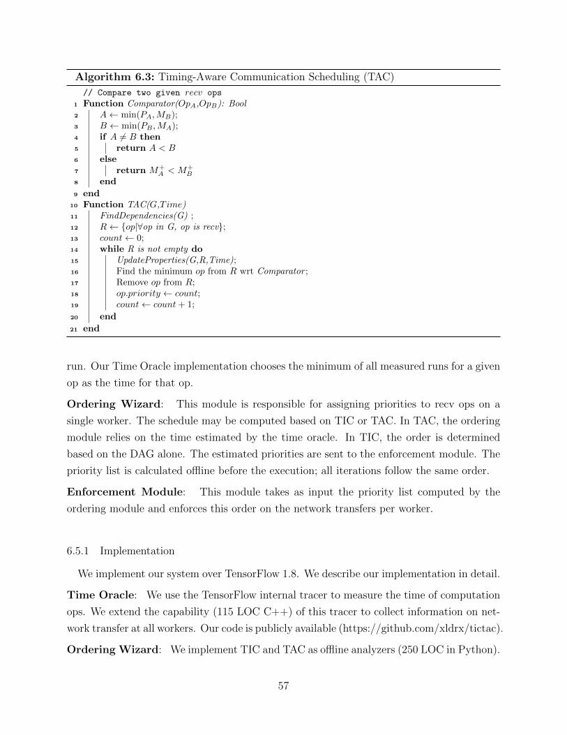
Algorithm 6.3: Timing-Aware Communication Scheduling (TAC)

// Compare two given recv ops

1 Function Comparator(OpA,OpB): Bool2 A← min(PA,MB);3 B ← min(PB ,MA);4 if A 6= B then5 return A < B6 else7 return M+

A < M+B

8 end

9 end10 Function TAC(G,Time)11 FindDependencies(G) ;12 R← {op|∀op in G, op is recv};13 count← 0;14 while R is not empty do15 UpdateProperties(G,R,Time);16 Find the minimum op from R wrt Comparator ;17 Remove op from R;18 op.priority ← count;19 count← count + 1;

20 end

21 end

run. Our Time Oracle implementation chooses the minimum of all measured runs for a given

op as the time for that op.

Ordering Wizard: This module is responsible for assigning priorities to recv ops on a

single worker. The schedule may be computed based on TIC or TAC. In TAC, the ordering

module relies on the time estimated by the time oracle. In TIC, the order is determined

based on the DAG alone. The estimated priorities are sent to the enforcement module. The

priority list is calculated offline before the execution; all iterations follow the same order.

Enforcement Module: This module takes as input the priority list computed by the

ordering module and enforces this order on the network transfers per worker.

6.5.1 Implementation

We implement our system over TensorFlow 1.8. We describe our implementation in detail.

Time Oracle: We use the TensorFlow internal tracer to measure the time of computation

ops. We extend the capability (115 LOC C++) of this tracer to collect information on net-

work transfer at all workers. Our code is publicly available (https://github.com/xldrx/tictac).

Ordering Wizard: We implement TIC and TAC as offline analyzers (250 LOC in Python).

57

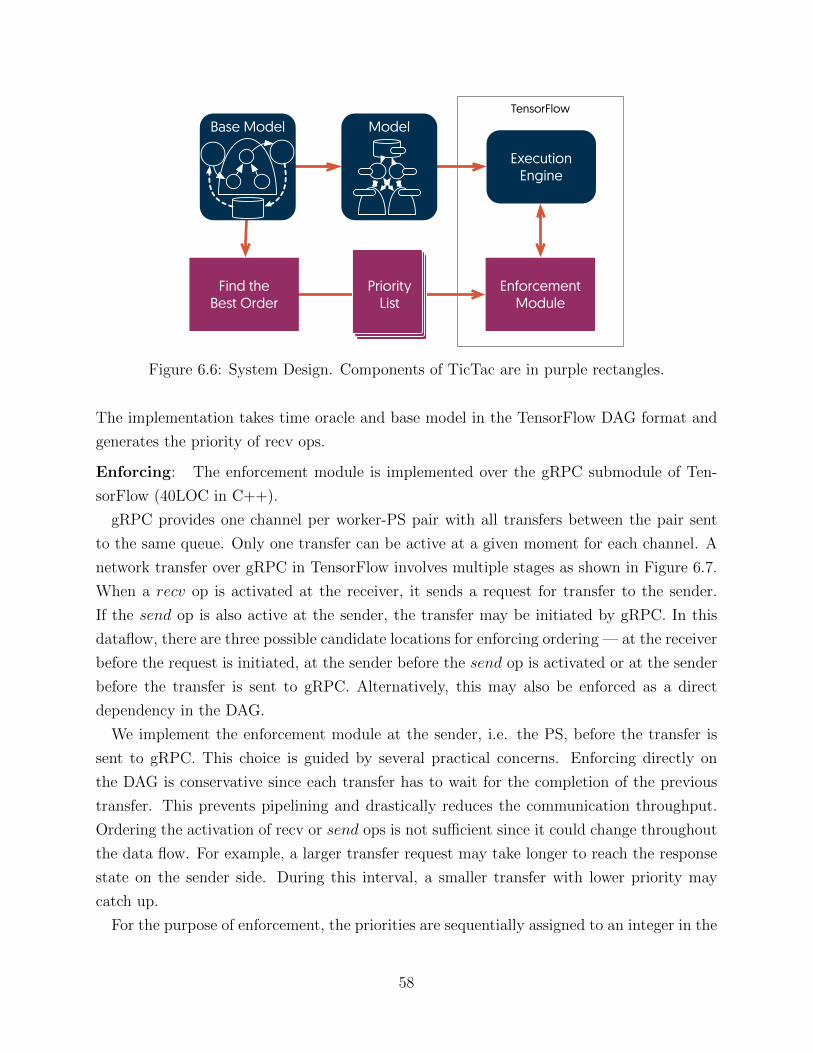
TensorFlow

Base Model Model

Find theBest Order

Enforcement Module

Execution Engine

Priority List

Figure 6.6: System Design. Components of TicTac are in purple rectangles.

The implementation takes time oracle and base model in the TensorFlow DAG format and

generates the priority of recv ops.

Enforcing: The enforcement module is implemented over the gRPC submodule of Ten-

sorFlow (40LOC in C++).

gRPC provides one channel per worker-PS pair with all transfers between the pair sent

to the same queue. Only one transfer can be active at a given moment for each channel. A

network transfer over gRPC in TensorFlow involves multiple stages as shown in Figure 6.7.

When a recv op is activated at the receiver, it sends a request for transfer to the sender.

If the send op is also active at the sender, the transfer may be initiated by gRPC. In this

dataflow, there are three possible candidate locations for enforcing ordering — at the receiver

before the request is initiated, at the sender before the send op is activated or at the sender

before the transfer is sent to gRPC. Alternatively, this may also be enforced as a direct

dependency in the DAG.

We implement the enforcement module at the sender, i.e. the PS, before the transfer is

sent to gRPC. This choice is guided by several practical concerns. Enforcing directly on

the DAG is conservative since each transfer has to wait for the completion of the previous

transfer. This prevents pipelining and drastically reduces the communication throughput.

Ordering the activation of recv or send ops is not sufficient since it could change throughout

the data flow. For example, a larger transfer request may take longer to reach the response

state on the sender side. During this interval, a smaller transfer with lower priority may

catch up.

For the purpose of enforcement, the priorities are sequentially assigned to an integer in the

58

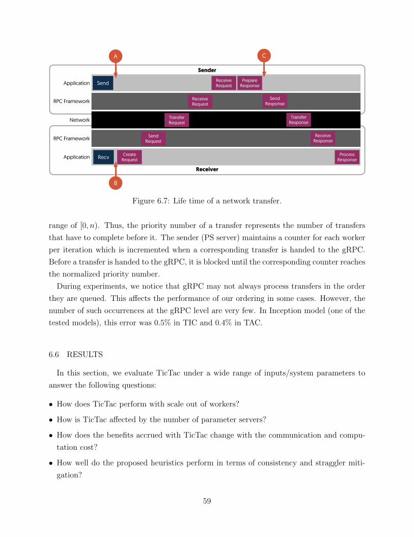
Receiver

Sender

Application

RPC Framework

Network

RPC Framework

Application

Recv

Send

Create Request

Send Request

TransferRequest

Receive Request

Receive Request

Prepare Response

Send Response

Process Response

Receive Response

TransferResponse

A C

B

Figure 6.7: Life time of a network transfer.

range of [0,n). Thus, the priority number of a transfer represents the number of transfers

that have to complete before it. The sender (PS server) maintains a counter for each worker

per iteration which is incremented when a corresponding transfer is handed to the gRPC.

Before a transfer is handed to the gRPC, it is blocked until the corresponding counter reaches

the normalized priority number.

During experiments, we notice that gRPC may not always process transfers in the order

they are queued. This affects the performance of our ordering in some cases. However, the

number of such occurrences at the gRPC level are very few. In Inception model (one of the

tested models), this error was 0.5% in TIC and 0.4% in TAC.

6.6 RESULTS

In this section, we evaluate TicTac under a wide range of inputs/system parameters to

answer the following questions:

• How does TicTac perform with scale out of workers?

• How is TicTac affected by the number of parameter servers?

• How does the benefits accrued with TicTac change with the communication and compu-

tation cost?

• How well do the proposed heuristics perform in terms of consistency and straggler miti-

gation?

59

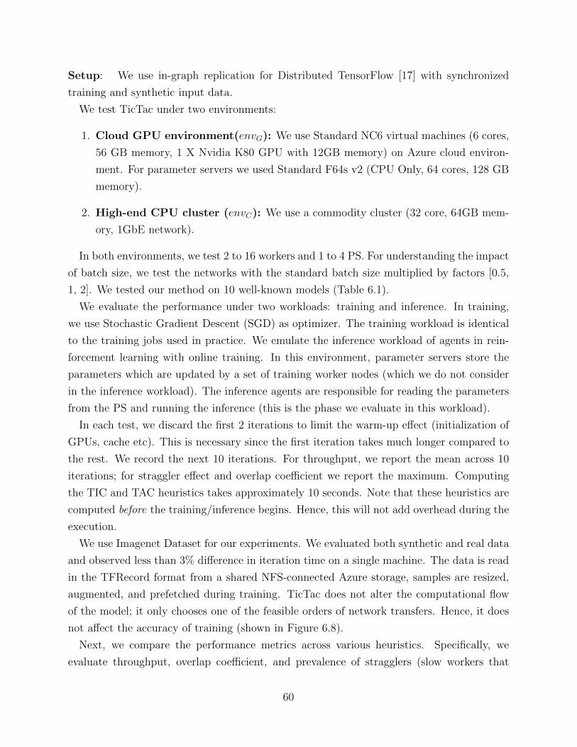
Setup: We use in-graph replication for Distributed TensorFlow [17] with synchronized

training and synthetic input data.

We test TicTac under two environments:

1. Cloud GPU environment(envG): We use Standard NC6 virtual machines (6 cores,

56 GB memory, 1 X Nvidia K80 GPU with 12GB memory) on Azure cloud environ-

ment. For parameter servers we used Standard F64s v2 (CPU Only, 64 cores, 128 GB

memory).

2. High-end CPU cluster (envC): We use a commodity cluster (32 core, 64GB mem-

ory, 1GbE network).

In both environments, we test 2 to 16 workers and 1 to 4 PS. For understanding the impact

of batch size, we test the networks with the standard batch size multiplied by factors [0.5,

1, 2]. We tested our method on 10 well-known models (Table 6.1).

We evaluate the performance under two workloads: training and inference. In training,

we use Stochastic Gradient Descent (SGD) as optimizer. The training workload is identical

to the training jobs used in practice. We emulate the inference workload of agents in rein-

forcement learning with online training. In this environment, parameter servers store the

parameters which are updated by a set of training worker nodes (which we do not consider

in the inference workload). The inference agents are responsible for reading the parameters

from the PS and running the inference (this is the phase we evaluate in this workload).

In each test, we discard the first 2 iterations to limit the warm-up effect (initialization of

GPUs, cache etc). This is necessary since the first iteration takes much longer compared to

the rest. We record the next 10 iterations. For throughput, we report the mean across 10

iterations; for straggler effect and overlap coefficient we report the maximum. Computing

the TIC and TAC heuristics takes approximately 10 seconds. Note that these heuristics are

computed before the training/inference begins. Hence, this will not add overhead during the

execution.

We use Imagenet Dataset for our experiments. We evaluated both synthetic and real data

and observed less than 3% difference in iteration time on a single machine. The data is read

in the TFRecord format from a shared NFS-connected Azure storage, samples are resized,

augmented, and prefetched during training. TicTac does not alter the computational flow

of the model; it only chooses one of the feasible orders of network transfers. Hence, it does

not affect the accuracy of training (shown in Figure 6.8).

Next, we compare the performance metrics across various heuristics. Specifically, we

evaluate throughput, overlap coefficient, and prevalence of stragglers (slow workers that

60

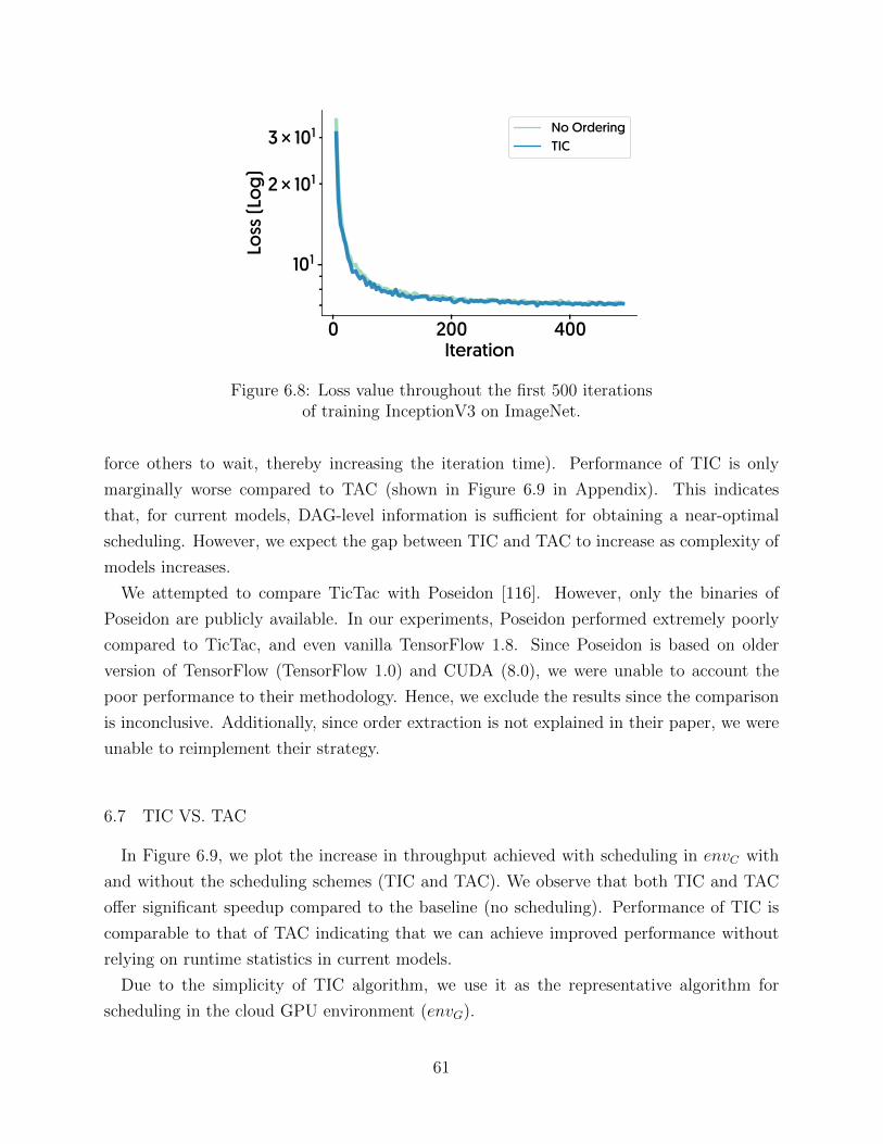
0 200 400Iteration

101

2 × 101

3 × 101

Loss

(Log

)

No OrderingTIC

Figure 6.8: Loss value throughout the first 500 iterationsof training InceptionV3 on ImageNet.

force others to wait, thereby increasing the iteration time). Performance of TIC is only

marginally worse compared to TAC (shown in Figure 6.9 in Appendix). This indicates

that, for current models, DAG-level information is sufficient for obtaining a near-optimal

scheduling. However, we expect the gap between TIC and TAC to increase as complexity of

models increases.

We attempted to compare TicTac with Poseidon [116]. However, only the binaries of

Poseidon are publicly available. In our experiments, Poseidon performed extremely poorly

compared to TicTac, and even vanilla TensorFlow 1.8. Since Poseidon is based on older

version of TensorFlow (TensorFlow 1.0) and CUDA (8.0), we were unable to account the

poor performance to their methodology. Hence, we exclude the results since the comparison

is inconclusive. Additionally, since order extraction is not explained in their paper, we were

unable to reimplement their strategy.

6.7 TIC VS. TAC

In Figure 6.9, we plot the increase in throughput achieved with scheduling in envC with

and without the scheduling schemes (TIC and TAC). We observe that both TIC and TAC

offer significant speedup compared to the baseline (no scheduling). Performance of TIC is

comparable to that of TAC indicating that we can achieve improved performance without

relying on runtime statistics in current models.

Due to the simplicity of TIC algorithm, we use it as the representative algorithm for

scheduling in the cloud GPU environment (envG).

61

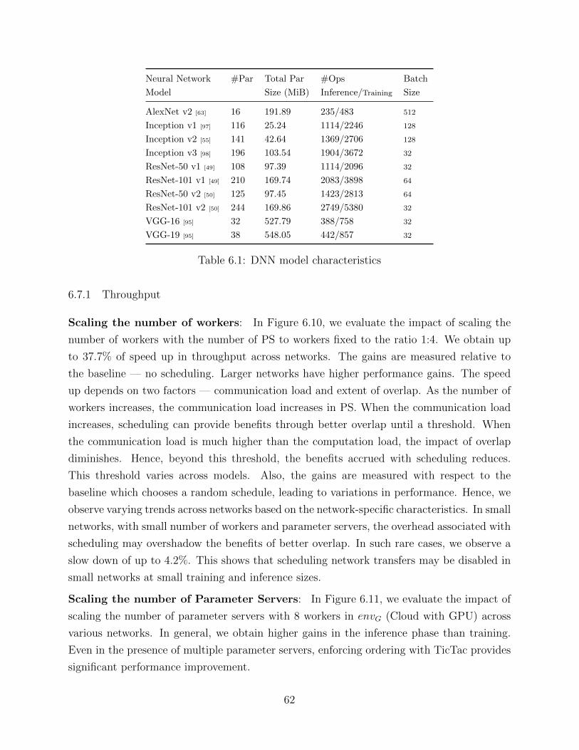
Neural Network

Model

#Par Total Par

Size (MiB)

#Ops

Inference/Training

Batch

Size

AlexNet v2 [63] 16 191.89 235/483 512

Inception v1 [97] 116 25.24 1114/2246 128

Inception v2 [55] 141 42.64 1369/2706 128

Inception v3 [98] 196 103.54 1904/3672 32

ResNet-50 v1 [49] 108 97.39 1114/2096 32

ResNet-101 v1 [49] 210 169.74 2083/3898 64

ResNet-50 v2 [50] 125 97.45 1423/2813 64

ResNet-101 v2 [50] 244 169.86 2749/5380 32

VGG-16 [95] 32 527.79 388/758 32

VGG-19 [95] 38 548.05 442/857 32

Table 6.1: DNN model characteristics

6.7.1 Throughput

Scaling the number of workers: In Figure 6.10, we evaluate the impact of scaling the

number of workers with the number of PS to workers fixed to the ratio 1:4. We obtain up

to 37.7% of speed up in throughput across networks. The gains are measured relative to

the baseline — no scheduling. Larger networks have higher performance gains. The speed

up depends on two factors — communication load and extent of overlap. As the number of

workers increases, the communication load increases in PS. When the communication load

increases, scheduling can provide benefits through better overlap until a threshold. When

the communication load is much higher than the computation load, the impact of overlap

diminishes. Hence, beyond this threshold, the benefits accrued with scheduling reduces.

This threshold varies across models. Also, the gains are measured with respect to the

baseline which chooses a random schedule, leading to variations in performance. Hence, we

observe varying trends across networks based on the network-specific characteristics. In small

networks, with small number of workers and parameter servers, the overhead associated with

scheduling may overshadow the benefits of better overlap. In such rare cases, we observe a

slow down of up to 4.2%. This shows that scheduling network transfers may be disabled in

small networks at small training and inference sizes.

Scaling the number of Parameter Servers: In Figure 6.11, we evaluate the impact of

scaling the number of parameter servers with 8 workers in envG (Cloud with GPU) across

various networks. In general, we obtain higher gains in the inference phase than training.

Even in the presence of multiple parameter servers, enforcing ordering with TicTac provides

significant performance improvement.

62

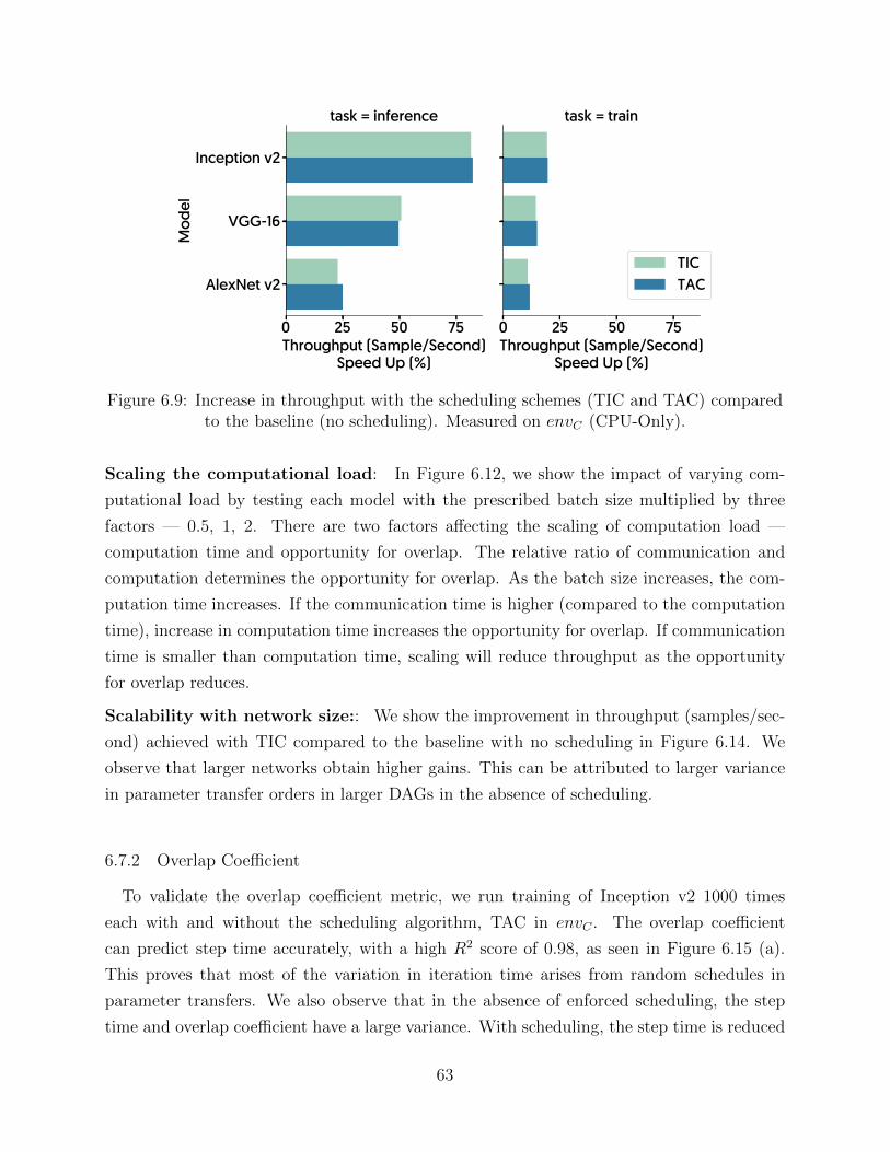
0 25 50 75Throughput (Sample/Second)

Speed Up (%)

Inception v2

VGG-16

AlexNet v2

Mod

el

task = inference

0 25 50 75Throughput (Sample/Second)

Speed Up (%)

task = train

TICTAC

Figure 6.9: Increase in throughput with the scheduling schemes (TIC and TAC) comparedto the baseline (no scheduling). Measured on envC (CPU-Only).

Scaling the computational load: In Figure 6.12, we show the impact of varying com-

putational load by testing each model with the prescribed batch size multiplied by three

factors — 0.5, 1, 2. There are two factors affecting the scaling of computation load —

computation time and opportunity for overlap. The relative ratio of communication and

computation determines the opportunity for overlap. As the batch size increases, the com-

putation time increases. If the communication time is higher (compared to the computation

time), increase in computation time increases the opportunity for overlap. If communication

time is smaller than computation time, scaling will reduce throughput as the opportunity

for overlap reduces.

Scalability with network size:: We show the improvement in throughput (samples/sec-

ond) achieved with TIC compared to the baseline with no scheduling in Figure 6.14. We

observe that larger networks obtain higher gains. This can be attributed to larger variance

in parameter transfer orders in larger DAGs in the absence of scheduling.

6.7.2 Overlap Coefficient

To validate the overlap coefficient metric, we run training of Inception v2 1000 times

each with and without the scheduling algorithm, TAC in envC . The overlap coefficient

can predict step time accurately, with a high R2 score of 0.98, as seen in Figure 6.15 (a).

This proves that most of the variation in iteration time arises from random schedules in

parameter transfers. We also observe that in the absence of enforced scheduling, the step

time and overlap coefficient have a large variance. With scheduling, the step time is reduced

63

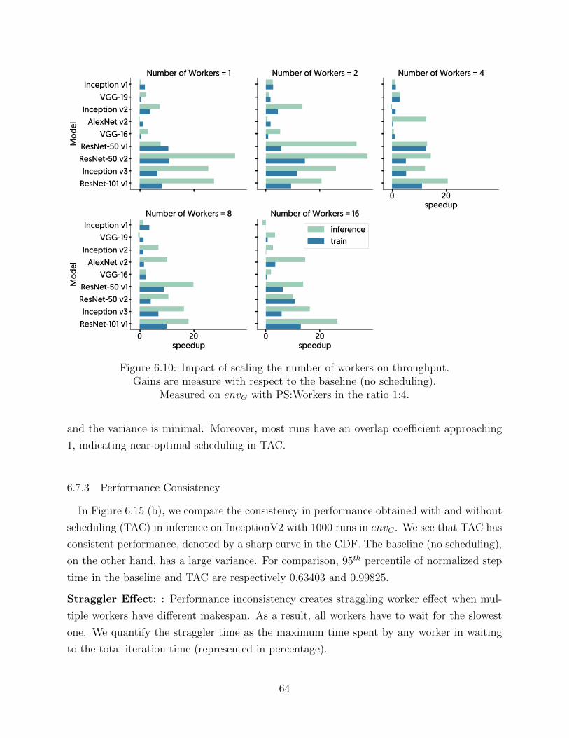
Inception v1VGG-19

Inception v2AlexNet v2

VGG-16ResNet-50 v1ResNet-50 v2Inception v3

ResNet-101 v1

Mod

elNumber of Workers = 1 Number of Workers = 2

0 20speedup

Number of Workers = 4

0 20speedup

Inception v1VGG-19

Inception v2AlexNet v2

VGG-16ResNet-50 v1ResNet-50 v2Inception v3

ResNet-101 v1

Mod

el

Number of Workers = 8

0 20speedup

Number of Workers = 16

inferencetrain

Figure 6.10: Impact of scaling the number of workers on throughput.Gains are measure with respect to the baseline (no scheduling).

Measured on envG with PS:Workers in the ratio 1:4.

and the variance is minimal. Moreover, most runs have an overlap coefficient approaching

1, indicating near-optimal scheduling in TAC.

6.7.3 Performance Consistency

In Figure 6.15 (b), we compare the consistency in performance obtained with and without

scheduling (TAC) in inference on InceptionV2 with 1000 runs in envC . We see that TAC has

consistent performance, denoted by a sharp curve in the CDF. The baseline (no scheduling),

on the other hand, has a large variance. For comparison, 95th percentile of normalized step

time in the baseline and TAC are respectively 0.63403 and 0.99825.

Straggler Effect: : Performance inconsistency creates straggling worker effect when mul-

tiple workers have different makespan. As a result, all workers have to wait for the slowest

one. We quantify the straggler time as the maximum time spent by any worker in waiting

to the total iteration time (represented in percentage).

64

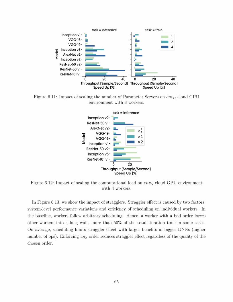
0 20 40Throughput (Sample/Second)

Speed Up (%)

Inception v1VGG-16VGG-19

Inception v3AlexNet v2

Inception v2ResNet-50 v2ResNet-50 v1ResNet-101 v1

Mod

el

task = inference

0 20 40Throughput (Sample/Second)

Speed Up (%)

task = train

124

Figure 6.11: Impact of scaling the number of Parameter Servers on envG cloud GPUenvironment with 8 workers.

0 20Throughput (Sample/Second)

Speed Up (%)

Inception v2ResNet-50 v1

AlexNet v2VGG-19VGG-16

Inception v1ResNet-50 v2Inception v3

ResNet-101 v1

Mod

el

task = inference

×12

×1×2

Figure 6.12: Impact of scaling the computational load on envG cloud GPU environmentwith 4 workers.

In Figure 6.13, we show the impact of stragglers. Straggler effect is caused by two factors:

system-level performance variations and efficiency of scheduling on individual workers. In

the baseline, workers follow arbitrary scheduling. Hence, a worker with a bad order forces

other workers into a long wait, more than 50% of the total iteration time in some cases.

On average, scheduling limits straggler effect with larger benefits in bigger DNNs (higher

number of ops). Enforcing any order reduces straggler effect regardless of the quality of the

chosen order.

65

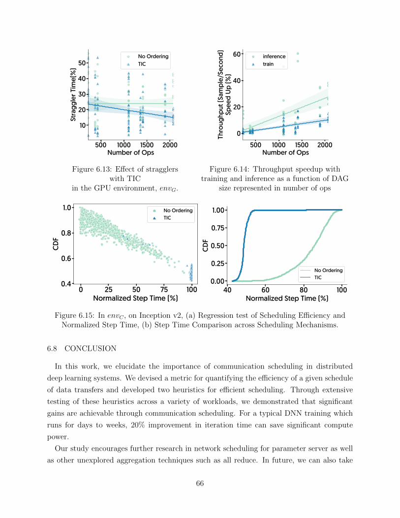
500 1000 1500 2000Number of Ops

10

20

30

40

50St

ragg

ler T

ime(

%)

No OrderingTIC

Figure 6.13: Effect of stragglerswith TIC

in the GPU environment, envG.

500 1000 1500 2000Number of Ops

0

20

40

60

Thro

ughp

ut (S

ampl

e/Se

cond

)Sp

eed

Up

(%)

inferencetrain

Figure 6.14: Throughput speedup withtraining and inference as a function of DAG

size represented in number of ops

0 25 50 75 100Normalized Step Time (%)

0.4

0.6

0.8

1.0

CD

F

No OrderingTIC

40 60 80 100Normalized Step Time (%)

0.00

0.25

0.50

0.75

1.00C

DF

No OrderingTIC

Figure 6.15: In envC , on Inception v2, (a) Regression test of Scheduling Efficiency andNormalized Step Time, (b) Step Time Comparison across Scheduling Mechanisms.

6.8 CONCLUSION

In this work, we elucidate the importance of communication scheduling in distributed

deep learning systems. We devised a metric for quantifying the efficiency of a given schedule

of data transfers and developed two heuristics for efficient scheduling. Through extensive

testing of these heuristics across a variety of workloads, we demonstrated that significant

gains are achievable through communication scheduling. For a typical DNN training which

runs for days to weeks, 20% improvement in iteration time can save significant compute

power.

Our study encourages further research in network scheduling for parameter server as well

as other unexplored aggregation techniques such as all reduce. In future, we can also take

66

into account additional metrics such as congestion from the network fabric for better net-

work performance. These results also provide motivation for extending the scheduling to

additional resources types such as memory and storage.

67

CHAPTER 7: ACHIEVING NETWORK EFFICIENCY THROUGHCOMPUTATION SCHEDULING

7.1 INTRODUCTION

Deep Neural Networks (DNNs) form the crux of advanced solutions in a variety of fields

such as computer vision and natural language processing. In frameworks such as Tensor-

Flow [1], interdependence of computation and communication operations involved in training

a model is represented using a dataflow graph which is a Directed Acyclic Graph (DAG).

The state of the DNN is represented by a vector of parameters. Each iteration involves

the computation of parameter updates, followed by its exchange between the participating

nodes.

Today, performance and scalability of distributed DNN training in the cloud is bottle-

necked by this parameter aggregation [52, 61]. Recently, decentralized aggregation schemes [13,

102, 32], initially introduced in the HPC environment [7, 89], have emerged as a popular

choice of aggregation in many frameworks [11, 90, 101]. In these schemes, unlike in the Pa-

rameter Server model, all workers store a copy of parameters which are aggregated through

collective transfers such as MPI allreduce() in MPI [40] or ncclAllReduce() in Nvidia’s

NCCL. However, in spite of recent optimizations [37], current decentralized implementa-

tions fail to achieve the guaranteed performance gains since they overlook interdependency

of communication and computation, especially in the cloud, which can leave GPUs idle for

a significant fraction of time.

In this paper, we introduce Caramel to improve efficiency of decentralized DNN train-

ing, in terms of iteration time and GPU utilization, through model-aware dataflow DAG

optimizations. Caramel achieves this goal by (a) expanding the feasible window of trans-

fer for each parameter (transfer boundaries) and (b) improving the network efficiency by

smoothening the load.

The transfer boundaries of a parameter represent the window when that parameter can

be aggregated without blocking the computation. When the transfer boundaries are farther

apart, the performance is less sensitive to slow network. Caramel expands these boundaries

through precise computation scheduling where it (i) moves the start boundaries earlier while

also reducing variance and (ii) pushes the end boundary by postponing the execution of

some computation operations to the next iteration.

Optimizations for smoothening the network load include (iii) batching of small parameters

to reduce the network overhead, and (iv) adaptive splitting and pipelining of parameters

to accelerate aggregation of large data which involves multi-stage network transfers with

68

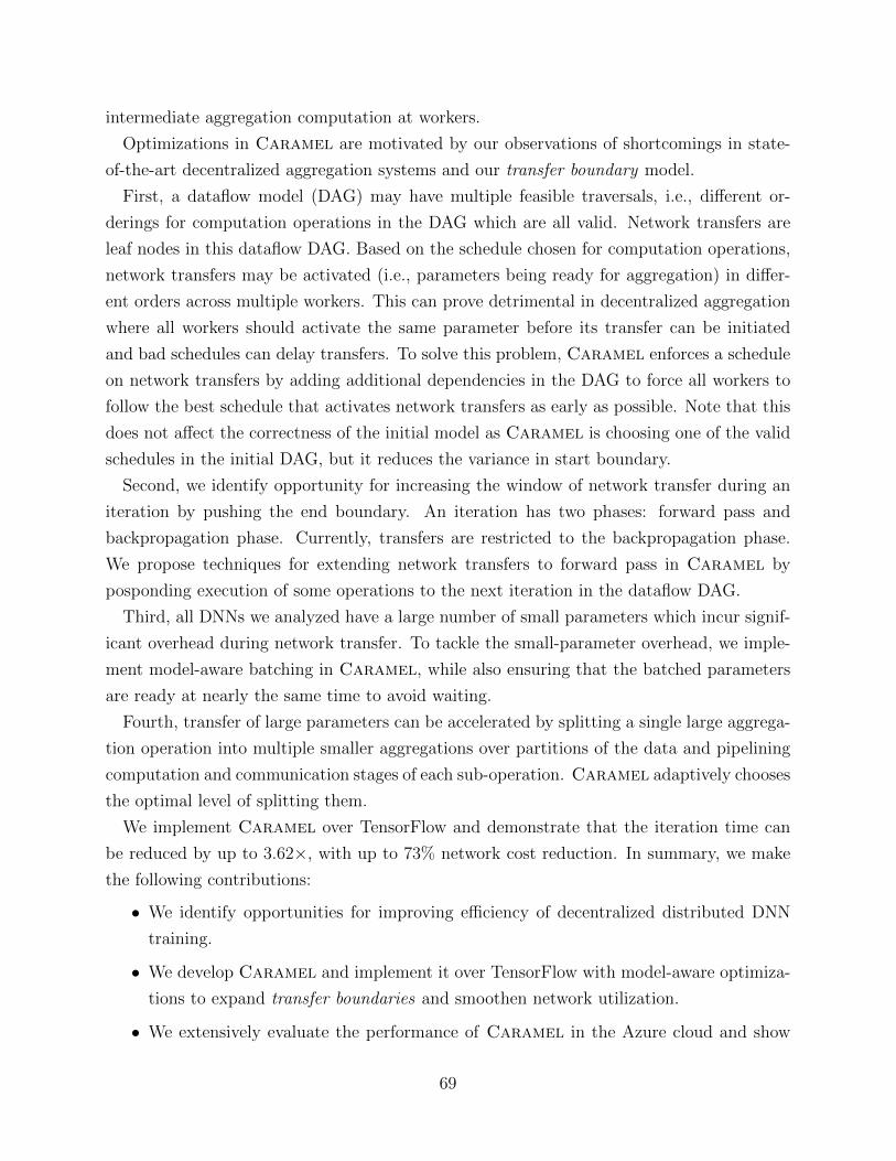
intermediate aggregation computation at workers.

Optimizations in Caramel are motivated by our observations of shortcomings in state-

of-the-art decentralized aggregation systems and our transfer boundary model.

First, a dataflow model (DAG) may have multiple feasible traversals, i.e., different or-

derings for computation operations in the DAG which are all valid. Network transfers are

leaf nodes in this dataflow DAG. Based on the schedule chosen for computation operations,

network transfers may be activated (i.e., parameters being ready for aggregation) in differ-

ent orders across multiple workers. This can prove detrimental in decentralized aggregation

where all workers should activate the same parameter before its transfer can be initiated

and bad schedules can delay transfers. To solve this problem, Caramel enforces a schedule

on network transfers by adding additional dependencies in the DAG to force all workers to

follow the best schedule that activates network transfers as early as possible. Note that this

does not affect the correctness of the initial model as Caramel is choosing one of the valid

schedules in the initial DAG, but it reduces the variance in start boundary.

Second, we identify opportunity for increasing the window of network transfer during an

iteration by pushing the end boundary. An iteration has two phases: forward pass and

backpropagation phase. Currently, transfers are restricted to the backpropagation phase.

We propose techniques for extending network transfers to forward pass in Caramel by

posponding execution of some operations to the next iteration in the dataflow DAG.

Third, all DNNs we analyzed have a large number of small parameters which incur signif-

icant overhead during network transfer. To tackle the small-parameter overhead, we imple-

ment model-aware batching in Caramel, while also ensuring that the batched parameters

are ready at nearly the same time to avoid waiting.

Fourth, transfer of large parameters can be accelerated by splitting a single large aggrega-

tion operation into multiple smaller aggregations over partitions of the data and pipelining

computation and communication stages of each sub-operation. Caramel adaptively chooses

the optimal level of splitting them.

We implement Caramel over TensorFlow and demonstrate that the iteration time can

be reduced by up to 3.62×, with up to 73% network cost reduction. In summary, we make

the following contributions:

• We identify opportunities for improving efficiency of decentralized distributed DNN

training.

• We develop Caramel and implement it over TensorFlow with model-aware optimiza-

tions to expand transfer boundaries and smoothen network utilization.

• We extensively evaluate the performance of Caramel in the Azure cloud and show

69

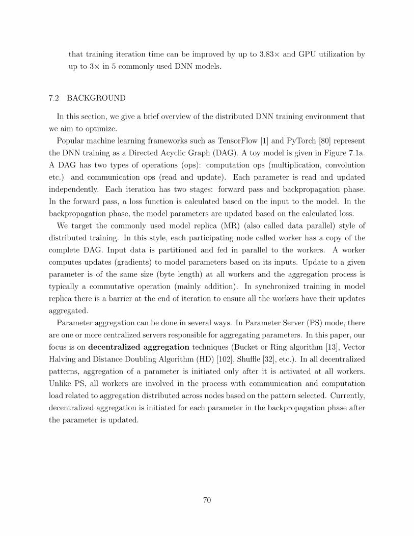
that training iteration time can be improved by up to 3.83× and GPU utilization by

up to 3× in 5 commonly used DNN models.

7.2 BACKGROUND

In this section, we give a brief overview of the distributed DNN training environment that

we aim to optimize.

Popular machine learning frameworks such as TensorFlow [1] and PyTorch [80] represent

the DNN training as a Directed Acyclic Graph (DAG). A toy model is given in Figure 7.1a.

A DAG has two types of operations (ops): computation ops (multiplication, convolution

etc.) and communication ops (read and update). Each parameter is read and updated

independently. Each iteration has two stages: forward pass and backpropagation phase.

In the forward pass, a loss function is calculated based on the input to the model. In the

backpropagation phase, the model parameters are updated based on the calculated loss.

We target the commonly used model replica (MR) (also called data parallel) style of

distributed training. In this style, each participating node called worker has a copy of the

complete DAG. Input data is partitioned and fed in parallel to the workers. A worker

computes updates (gradients) to model parameters based on its inputs. Update to a given

parameter is of the same size (byte length) at all workers and the aggregation process is

typically a commutative operation (mainly addition). In synchronized training in model

replica there is a barrier at the end of iteration to ensure all the workers have their updates

aggregated.

Parameter aggregation can be done in several ways. In Parameter Server (PS) mode, there

are one or more centralized servers responsible for aggregating parameters. In this paper, our

focus is on decentralized aggregation techniques (Bucket or Ring algorithm [13], Vector

Halving and Distance Doubling Algorithm (HD) [102], Shuffle [32], etc.). In all decentralized

patterns, aggregation of a parameter is initiated only after it is activated at all workers.

Unlike PS, all workers are involved in the process with communication and computation

load related to aggregation distributed across nodes based on the pattern selected. Currently,

decentralized aggregation is initiated for each parameter in the backpropagation phase after

the parameter is updated.

70

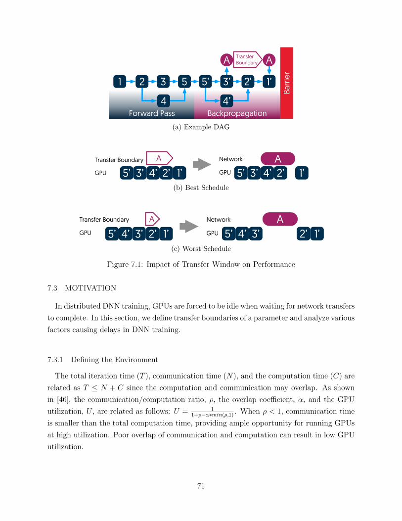
Forward Pass Backpropagation

Transfer Boundary

Barr

ier

5’ 2’2

4’

53

4

3’ 1’1

A A

(a) Example DAG

5’ 3’ 4’ 2’ 1’ ATransfer Boundary

GPU

A5’ 3’ 4’ 2’ 1’

Network

GPU

(b) Best Schedule

5’ 4’ 3’ 2’ 1’ ATransfer Boundary

GPU

A5’ 4’ 3’ 2’ 1’

Network

GPU

(c) Worst Schedule

Figure 7.1: Impact of Transfer Window on Performance

7.3 MOTIVATION

In distributed DNN training, GPUs are forced to be idle when waiting for network transfers

to complete. In this section, we define transfer boundaries of a parameter and analyze various

factors causing delays in DNN training.

7.3.1 Defining the Environment

The total iteration time (T ), communication time (N), and the computation time (C) are

related as T ≤ N + C since the computation and communication may overlap. As shown

in [46], the communication/computation ratio, ρ, the overlap coefficient, α, and the GPU

utilization, U , are related as follows: U = 11+ρ−α∗min(ρ,1) . When ρ < 1, communication time

is smaller than the total computation time, providing ample opportunity for running GPUs

at high utilization. Poor overlap of communication and computation can result in low GPU

utilization.

71

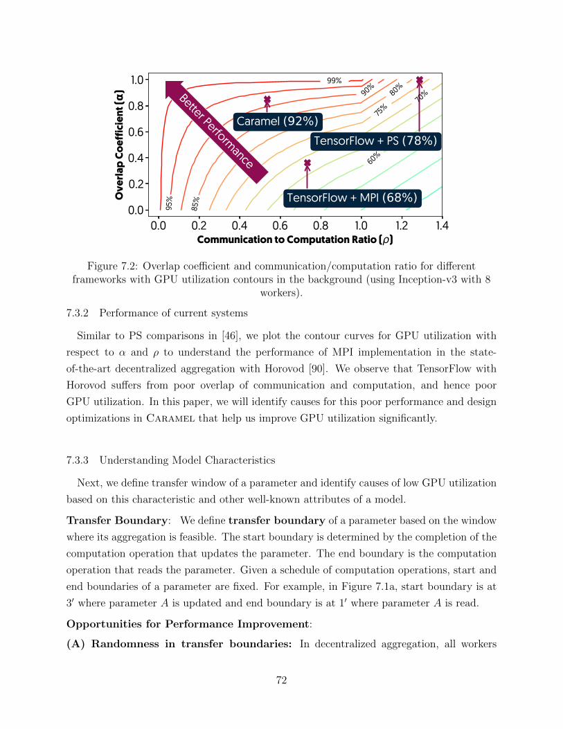
0.0 0.2 0.4 0.6 0.8 1.0 1.2 1.4Communication to Computation Ratio ( )

0.0

0.2

0.4

0.6

0.8

1.0

Ove

rlap

Coef

ficie

nt (

)

TensorFlow + MPI (68%)

TensorFlow + PS (78%)Caramel (92%)

Better Performance

35%

40%

45%

50%

55%

60%

65%

70%

75%

80%

85%

90%

95%

99%

Figure 7.2: Overlap coefficient and communication/computation ratio for differentframeworks with GPU utilization contours in the background (using Inception-v3 with 8

workers).

7.3.2 Performance of current systems

Similar to PS comparisons in [46], we plot the contour curves for GPU utilization with

respect to α and ρ to understand the performance of MPI implementation in the state-

of-the-art decentralized aggregation with Horovod [90]. We observe that TensorFlow with

Horovod suffers from poor overlap of communication and computation, and hence poor

GPU utilization. In this paper, we will identify causes for this poor performance and design

optimizations in Caramel that help us improve GPU utilization significantly.

7.3.3 Understanding Model Characteristics

Next, we define transfer window of a parameter and identify causes of low GPU utilization

based on this characteristic and other well-known attributes of a model.

Transfer Boundary: We define transfer boundary of a parameter based on the window

where its aggregation is feasible. The start boundary is determined by the completion of the

computation operation that updates the parameter. The end boundary is the computation

operation that reads the parameter. Given a schedule of computation operations, start and

end boundaries of a parameter are fixed. For example, in Figure 7.1a, start boundary is at

3′ where parameter A is updated and end boundary is at 1′ where parameter A is read.

Opportunities for Performance Improvement:

(A) Randomness in transfer boundaries: In decentralized aggregation, all workers

72

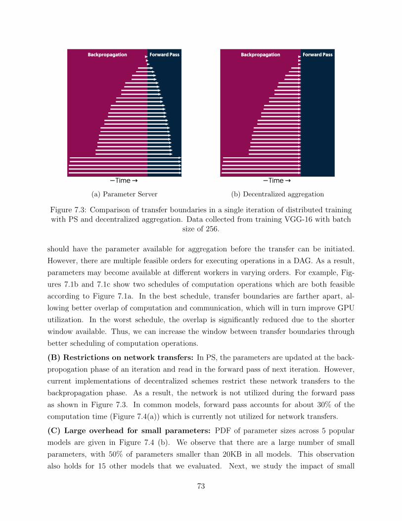
Time

Backpropagation Forward Pass

(a) Parameter Server

Time

Backpropagation Forward Pass

(b) Decentralized aggregation

Figure 7.3: Comparison of transfer boundaries in a single iteration of distributed trainingwith PS and decentralized aggregation. Data collected from training VGG-16 with batch

size of 256.

should have the parameter available for aggregation before the transfer can be initiated.

However, there are multiple feasible orders for executing operations in a DAG. As a result,

parameters may become available at different workers in varying orders. For example, Fig-

ures 7.1b and 7.1c show two schedules of computation operations which are both feasible

according to Figure 7.1a. In the best schedule, transfer boundaries are farther apart, al-

lowing better overlap of computation and communication, which will in turn improve GPU

utilization. In the worst schedule, the overlap is significantly reduced due to the shorter

window available. Thus, we can increase the window between transfer boundaries through

better scheduling of computation operations.

(B) Restrictions on network transfers: In PS, the parameters are updated at the back-

propogation phase of an iteration and read in the forward pass of next iteration. However,

current implementations of decentralized schemes restrict these network transfers to the

backpropagation phase. As a result, the network is not utilized during the forward pass

as shown in Figure 7.3. In common models, forward pass accounts for about 30% of the

computation time (Figure 7.4(a)) which is currently not utilized for network transfers.

(C) Large overhead for small parameters: PDF of parameter sizes across 5 popular

models are given in Figure 7.4 (b). We observe that there are a large number of small

parameters, with 50% of parameters smaller than 20KB in all models. This observation

also holds for 15 other models that we evaluated. Next, we study the impact of small

73

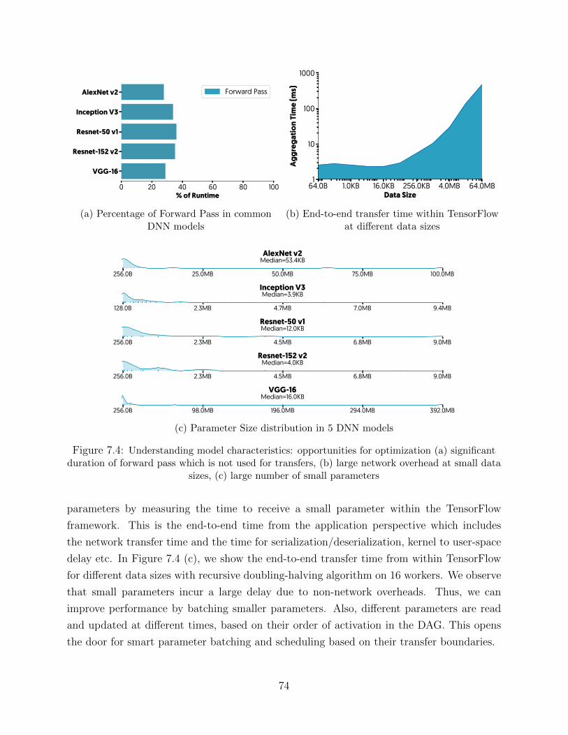
0 20 40 60 80 100% of Runtime

AlexNet v2

Inception V3

Resnet-50 v1

Resnet-152 v2

VGG-16

Forward Pass

(a) Percentage of Forward Pass in commonDNN models

64.0B 1.0KB 16.0KB 256.0KB 4.0MB 64.0MBData Size

1

10

100

1000

Agg

rega

tion

Tim

e (m

s)

(b) End-to-end transfer time within TensorFlowat different data sizes

256.0B 25.0MB 50.0MB 75.0MB 100.0MB

Median=53.4KBAlexNet v2

128.0B 2.3MB 4.7MB 7.0MB 9.4MB

Median=3.9KBInception V3

256.0B 2.3MB 4.5MB 6.8MB 9.0MB

Median=12.0KBResnet-50 v1

256.0B 2.3MB 4.5MB 6.8MB 9.0MB

Median=4.0KBResnet-152 v2

256.0B 98.0MB 196.0MB 294.0MB 392.0MB

Median=16.0KBVGG-16

(c) Parameter Size distribution in 5 DNN models

Figure 7.4: Understanding model characteristics: opportunities for optimization (a) significantduration of forward pass which is not used for transfers, (b) large network overhead at small data

sizes, (c) large number of small parameters

parameters by measuring the time to receive a small parameter within the TensorFlow

framework. This is the end-to-end time from the application perspective which includes

the network transfer time and the time for serialization/deserialization, kernel to user-space

delay etc. In Figure 7.4 (c), we show the end-to-end transfer time from within TensorFlow

for different data sizes with recursive doubling-halving algorithm on 16 workers. We observe

that small parameters incur a large delay due to non-network overheads. Thus, we can

improve performance by batching smaller parameters. Also, different parameters are read

and updated at different times, based on their order of activation in the DAG. This opens

the door for smart parameter batching and scheduling based on their transfer boundaries.

74

5’ 2’

4’

3’ 1’

A

(a) Before

5’ 2’

4’

3’ 1’

A

(b) After

Figure 7.5: DAG Optimization in Caramel

7.4 Caramel DESIGN

Network transfer optimization in Caramel involves four functionalities: (i) dataflow DAG

optimizer, (ii) small-parameter batcher, (iii) network transfer scheduler, and (iv) adaptive

depth enforcer.

7.4.1 Dataflow DAG Optimizer

In decentralized aggregation patterns, it is necessary to have a parameter ready for ag-

gregation at all workers before it can be aggregated (§ 7.3.3 B). This module is responsible

for (i) determining the best executing order of ops in the DAG and (ii) adding additional

dependencies in the model to ensure that there is only a single feasible order of execution.

Stage 1 — Determining the best order: To maximize the overlap coefficient, α, the

computations should be prioritized in a manner that activates the communication operations

as early as possible (early start boundary for parameters). We add the minimal number of

additional dependencies to ensure desired ordering on the parameter updates/activation.

First, we trace execution of an iteration on a single machine 10 times. The execution

time of a computation operation is determined as the minimum observed time across all

runs. Empirically, we find that our method can accurately predict the computation time of

execution (with less than 3% error in the worst case) with only 5 runs.

Next, we use an iterative greedy algorithm to find the best order of parameter updates. In

each step, we calculate the total time taken by computation ops that need to be completed

before each parameter can be activated. The parameter with the least cost of computation

required to activate it is chosen and the computation ops that it depends on are marked as

completed (their are not counted as dependencies in the next iterations). This process is

repeated until all parameter updates are visited.

75

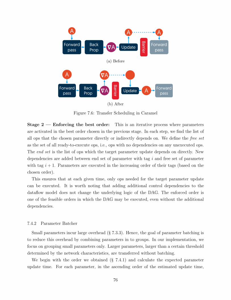
Forward pass

A

Back Prop

Update

Barrier!A

A A

Forward pass

(a) Before

Forward pass

A

Back Prop Update

Barrier!A

!A

Forward passA

(b) After

Figure 7.6: Transfer Scheduling in Caramel

Stage 2 — Enforcing the best order: This is an iterative process where parameters

are activated in the best order chosen in the previous stage. In each step, we find the list of

all ops that the chosen parameter directly or indirectly depends on. We define the free set

as the set of all ready-to-execute ops, i.e., ops with no dependencies on any unexecuted ops.

The end set is the list of ops which the target parameter update depends on directly. New

dependencies are added between end set of parameter with tag i and free set of parameter

with tag i + 1. Parameters are executed in the increasing order of their tags (based on the

chosen order).

This ensures that at each given time, only ops needed for the target parameter update

can be executed. It is worth noting that adding additional control dependencies to the

dataflow model does not change the underlying logic of the DAG. The enforced order is

one of the feasible orders in which the DAG may be executed, even without the additional

dependencies.

7.4.2 Parameter Batcher

Small parameters incur large overhead (§ 7.3.3). Hence, the goal of parameter batching is

to reduce this overhead by combining parameters in to groups. In our implementation, we

focus on grouping small parameters only. Larger parameters, larger than a certain threshold

determined by the network characteristics, are transferred without batching.

We begin with the order we obtained (§ 7.4.1) and calculate the expected parameter

update time. For each parameter, in the ascending order of the estimated update time,

76

we determine whether to batch it or not. If the size of the parameter is larger than the

threshold (the choice of the threshold explained in the next paragraph), it is transferred

without batching. If the parameter is smaller than the threshold, we decide whether to

transfer immediately (effectively, putting the transfer in a queue to transfer eventually) or

add to the current active batch. The current batch is transferred when the active batch size

exceeds the threshold or if the transfers in the queue are done before the next parameter

update.

This algorithm ensures that parameters are batched whenever there is an opportunity,

i.e., the network is busy with other transfers. The threshold plays an important role in this

algorithm. If the threshold is too small, too few parameters will be batched. If it is too

large, the batching overhead will exceed the benefit. The threshold can be set manually.

We use a network model to predict the total transfer time for a given data size. Empirically,

we find that a simple linear regression model can accurately predict the transfer time for a

given data size in the network. In order to generate this model, we run two sets of network

microbenchmarks for two data sizes: 64B, and 4MB. The choice of data size is arbitrary;

we get very similar results with different combinations. For each chosen data size, we run

sequential aggregation transfers and record the time. Next, we fit this data to a linear model.

Using this network model, we estimate the best threshold as follows:

Threshold = minxf(2x)

2f(x)> 0.8 (7.1)

where f(d) is the network transfer time for data size d. We obtain the minimum overhead

using this threshold.

7.4.3 Network Transfer Scheduler

The network transfer scheduler is responsible for increasing the overlap coefficient by

scheduling parameter transfers efficiently. Transfers are scheduled in both backward pass

and forward pass to overcome the shortcomings discussed in § 7.3.3, without affecting the

computation (Figure 7.6).

Moving a network transfer to the forward pass has the possibility of causing delay in com-

putation. We avoid this problem through model-awareness. A parameter cannot be updated

beyond its transfer boundaries. For batched parameters, this boundary is determined by the

parameter that is read at the earliest time/updated at the latest time.

We implement a greedy 2D-Bin packing algorithm to pack the parameters based on their

feasible window. The two dimensions are time and data size. The algorithm proceeds as

77

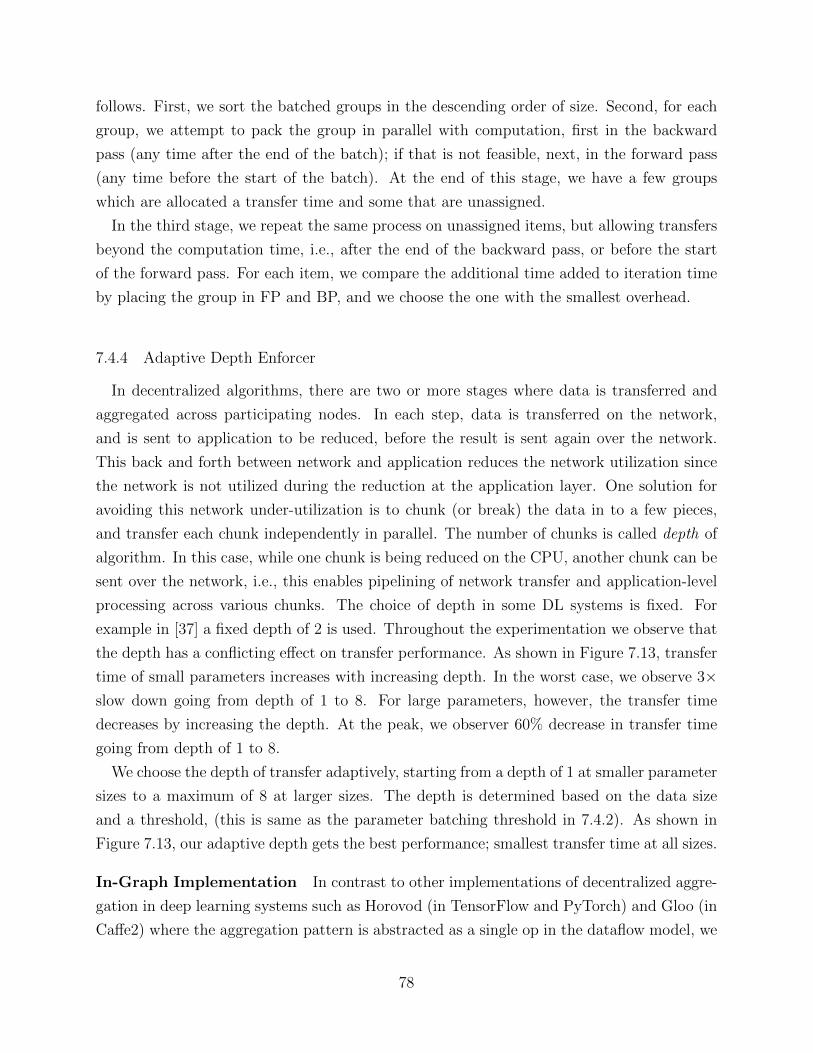
follows. First, we sort the batched groups in the descending order of size. Second, for each

group, we attempt to pack the group in parallel with computation, first in the backward

pass (any time after the end of the batch); if that is not feasible, next, in the forward pass

(any time before the start of the batch). At the end of this stage, we have a few groups

which are allocated a transfer time and some that are unassigned.

In the third stage, we repeat the same process on unassigned items, but allowing transfers

beyond the computation time, i.e., after the end of the backward pass, or before the start

of the forward pass. For each item, we compare the additional time added to iteration time

by placing the group in FP and BP, and we choose the one with the smallest overhead.

7.4.4 Adaptive Depth Enforcer

In decentralized algorithms, there are two or more stages where data is transferred and

aggregated across participating nodes. In each step, data is transferred on the network,

and is sent to application to be reduced, before the result is sent again over the network.

This back and forth between network and application reduces the network utilization since

the network is not utilized during the reduction at the application layer. One solution for

avoiding this network under-utilization is to chunk (or break) the data in to a few pieces,

and transfer each chunk independently in parallel. The number of chunks is called depth of

algorithm. In this case, while one chunk is being reduced on the CPU, another chunk can be

sent over the network, i.e., this enables pipelining of network transfer and application-level

processing across various chunks. The choice of depth in some DL systems is fixed. For

example in [37] a fixed depth of 2 is used. Throughout the experimentation we observe that

the depth has a conflicting effect on transfer performance. As shown in Figure 7.13, transfer

time of small parameters increases with increasing depth. In the worst case, we observe 3×slow down going from depth of 1 to 8. For large parameters, however, the transfer time

decreases by increasing the depth. At the peak, we observer 60% decrease in transfer time

going from depth of 1 to 8.

We choose the depth of transfer adaptively, starting from a depth of 1 at smaller parameter

sizes to a maximum of 8 at larger sizes. The depth is determined based on the data size

and a threshold, (this is same as the parameter batching threshold in 7.4.2). As shown in

Figure 7.13, our adaptive depth gets the best performance; smallest transfer time at all sizes.

In-Graph Implementation In contrast to other implementations of decentralized aggre-

gation in deep learning systems such as Horovod (in TensorFlow and PyTorch) and Gloo (in

Caffe2) where the aggregation pattern is abstracted as a single op in the dataflow model, we

78

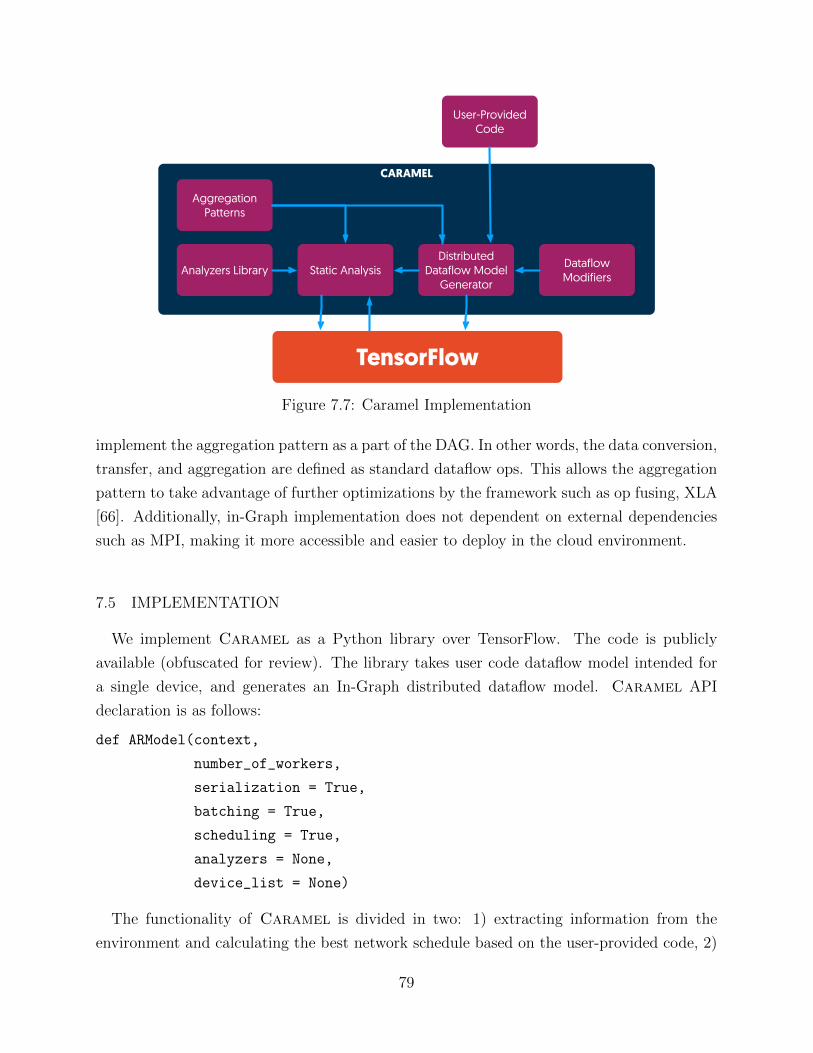
CARAMEL

Static AnalysisDistributed

Dataflow Model Generator

User-Provided Code

TensorFlow

Analyzers Library Dataflow Modifiers

Aggregation Patterns

Figure 7.7: Caramel Implementation

implement the aggregation pattern as a part of the DAG. In other words, the data conversion,

transfer, and aggregation are defined as standard dataflow ops. This allows the aggregation

pattern to take advantage of further optimizations by the framework such as op fusing, XLA

[66]. Additionally, in-Graph implementation does not dependent on external dependencies

such as MPI, making it more accessible and easier to deploy in the cloud environment.

7.5 IMPLEMENTATION

We implement Caramel as a Python library over TensorFlow. The code is publicly

available (obfuscated for review). The library takes user code dataflow model intended for

a single device, and generates an In-Graph distributed dataflow model. Caramel API

declaration is as follows:

def ARModel(context,

number_of_workers,

serialization = True,

batching = True,

scheduling = True,

analyzers = None,

device_list = None)

The functionality of Caramel is divided in two: 1) extracting information from the

environment and calculating the best network schedule based on the user-provided code, 2)

79

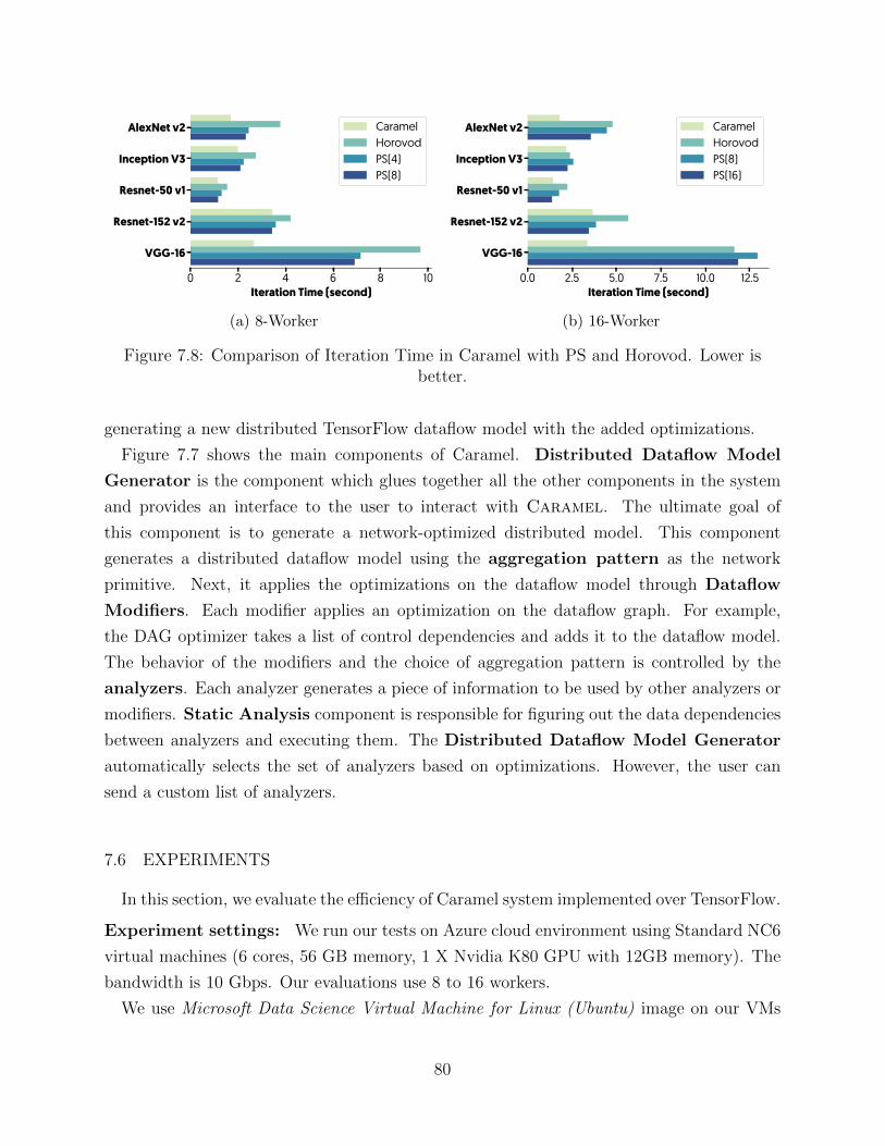
0 2 4 6 8 10Iteration Time (second)

AlexNet v2

Inception V3

Resnet-50 v1

Resnet-152 v2

VGG-16

CaramelHorovodPS(4)PS(8)

(a) 8-Worker

0.0 2.5 5.0 7.5 10.0 12.5Iteration Time (second)

AlexNet v2

Inception V3

Resnet-50 v1

Resnet-152 v2

VGG-16

CaramelHorovodPS(8)PS(16)

(b) 16-Worker

Figure 7.8: Comparison of Iteration Time in Caramel with PS and Horovod. Lower isbetter.

generating a new distributed TensorFlow dataflow model with the added optimizations.

Figure 7.7 shows the main components of Caramel. Distributed Dataflow Model

Generator is the component which glues together all the other components in the system

and provides an interface to the user to interact with Caramel. The ultimate goal of

this component is to generate a network-optimized distributed model. This component

generates a distributed dataflow model using the aggregation pattern as the network

primitive. Next, it applies the optimizations on the dataflow model through Dataflow

Modifiers. Each modifier applies an optimization on the dataflow graph. For example,

the DAG optimizer takes a list of control dependencies and adds it to the dataflow model.

The behavior of the modifiers and the choice of aggregation pattern is controlled by the

analyzers. Each analyzer generates a piece of information to be used by other analyzers or

modifiers. Static Analysis component is responsible for figuring out the data dependencies

between analyzers and executing them. The Distributed Dataflow Model Generator

automatically selects the set of analyzers based on optimizations. However, the user can

send a custom list of analyzers.

7.6 EXPERIMENTS

In this section, we evaluate the efficiency of Caramel system implemented over TensorFlow.

Experiment settings: We run our tests on Azure cloud environment using Standard NC6

virtual machines (6 cores, 56 GB memory, 1 X Nvidia K80 GPU with 12GB memory). The

bandwidth is 10 Gbps. Our evaluations use 8 to 16 workers.

We use Microsoft Data Science Virtual Machine for Linux (Ubuntu) image on our VMs

80

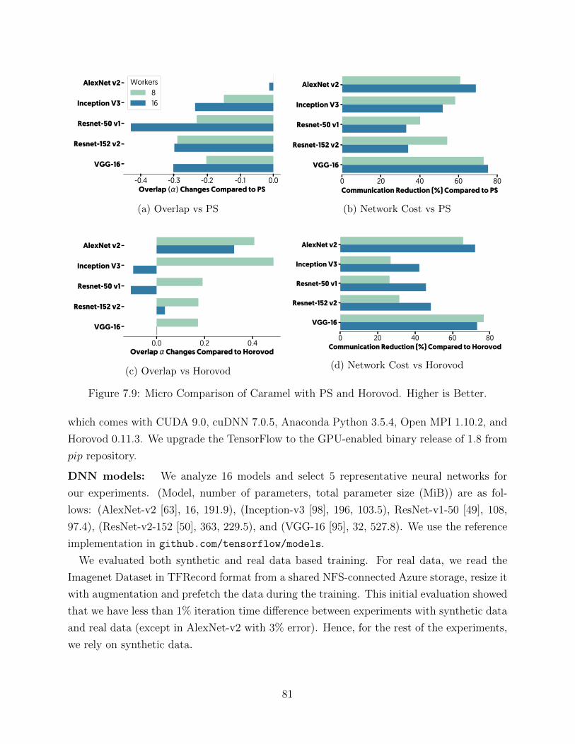
-0.4 -0.3 -0.2 -0.1 0.0Overlap ( ) Changes Compared to PS

AlexNet v2

Inception V3

Resnet-50 v1

Resnet-152 v2

VGG-16

Workers816

(a) Overlap vs PS

0 20 40 60 80Communication Reduction (%) Compared to PS

AlexNet v2

Inception V3

Resnet-50 v1

Resnet-152 v2

VGG-16

(b) Network Cost vs PS

0.0 0.2 0.4Overlap Changes Compared to Horovod

AlexNet v2

Inception V3

Resnet-50 v1

Resnet-152 v2

VGG-16

(c) Overlap vs Horovod

0 20 40 60 80Communication Reduction (%) Compared to Horovod

AlexNet v2

Inception V3

Resnet-50 v1

Resnet-152 v2

VGG-16

(d) Network Cost vs Horovod

Figure 7.9: Micro Comparison of Caramel with PS and Horovod. Higher is Better.

which comes with CUDA 9.0, cuDNN 7.0.5, Anaconda Python 3.5.4, Open MPI 1.10.2, and

Horovod 0.11.3. We upgrade the TensorFlow to the GPU-enabled binary release of 1.8 from

pip repository.

DNN models: We analyze 16 models and select 5 representative neural networks for

our experiments. (Model, number of parameters, total parameter size (MiB)) are as fol-

lows: (AlexNet-v2 [63], 16, 191.9), (Inception-v3 [98], 196, 103.5), ResNet-v1-50 [49], 108,

97.4), (ResNet-v2-152 [50], 363, 229.5), and (VGG-16 [95], 32, 527.8). We use the reference

implementation in github.com/tensorflow/models.

We evaluated both synthetic and real data based training. For real data, we read the

Imagenet Dataset in TFRecord format from a shared NFS-connected Azure storage, resize it

with augmentation and prefetch the data during the training. This initial evaluation showed

that we have less than 1% iteration time difference between experiments with synthetic data

and real data (except in AlexNet-v2 with 3% error). Hence, for the rest of the experiments,

we rely on synthetic data.

81

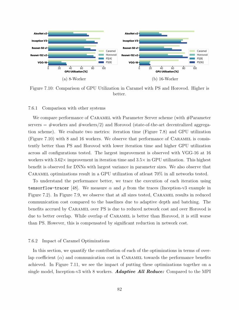
0 20 40 60 80 100GPU Utilization (%)

AlexNet v2

Inception V3

Resnet-50 v1

Resnet-152 v2

VGG-16

CaramelHorovodPS(4)PS(8)

(a) 8-Worker

0 20 40 60 80 100GPU Utilization (%)

AlexNet v2

Inception V3

Resnet-50 v1

Resnet-152 v2

VGG-16

CaramelHorovodPS(8)PS(16)

(b) 16-Worker

Figure 7.10: Comparison of GPU Utilization in Caramel with PS and Horovod. Higher isbetter.

7.6.1 Comparison with other systems

We compare performance of Caramel with Parameter Server scheme (with #Parameter

servers = #workers and #workers/2) and Horovod (state-of-the-art decentralized aggrega-

tion scheme). We evaluate two metrics: iteration time (Figure 7.8) and GPU utilization

(Figure 7.10) with 8 and 16 workers. We observe that performance of Caramel is consis-

tently better than PS and Horovod with lower iteration time and higher GPU utilization

across all configurations tested. The largest improvement is observed with VGG-16 at 16

workers with 3.62× improvement in iteration time and 3.5× in GPU utilization. This highest

benefit is observed for DNNs with largest variance in parameter sizes. We also observe that

Caramel optimizations result in a GPU utilization of atleast 70% in all networks tested.

To understand the performance better, we trace the execution of each iteration using

tensorflow-tracer [48]. We measure α and ρ from the traces (Inception-v3 example in

Figure 7.2). In Figure 7.9, we observe that at all sizes tested, Caramel results in reduced

communication cost compared to the baselines due to adaptive depth and batching. The

benefits accrued by Caramel over PS is due to reduced network cost and over Horovod is

due to better overlap. While overlap of Caramel is better than Horovod, it is still worse

than PS. However, this is compensated by significant reduction in network cost.

7.6.2 Impact of Caramel Optimizations

In this section, we quantify the contribution of each of the optimizations in terms of over-

lap coefficient (α) and communication cost in Caramel towards the performance benefits

achieved. In Figure 7.11, we see the impact of putting these optimizations together on a

single model, Inception-v3 with 8 workers. Adaptive All Reduce: Compared to the MPI

82

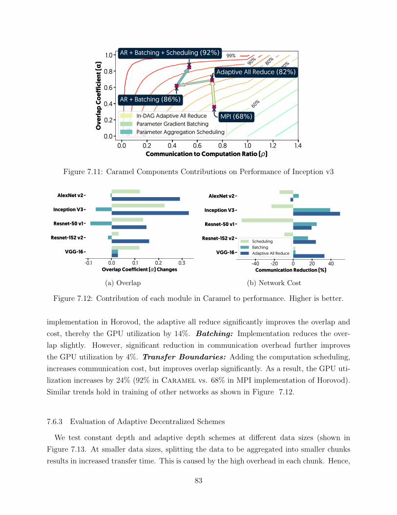
0.0 0.2 0.4 0.6 0.8 1.0 1.2 1.4Communication to Computation Ratio ( )

0.0

0.2

0.4

0.6

0.8

1.0

Ove

rlap

Coef

ficie

nt (

)

35%

40%

45%

50%

55%

60%

65%

70%

75%

80%

85%

90%

95%

99%

In-DAG Adaptive All ReduceParameter Gradient BatchingParameter Aggregation Scheduling

MPI (68%)

AR + Batching + Scheduling (92%)

Adaptive All Reduce (82%)

AR + Batching (86%)

Figure 7.11: Caramel Components Contributions on Performance of Inception v3

-0.1 0.0 0.1 0.2 0.3Overlap Coefficient ( ) Changes

AlexNet v2

Inception V3

Resnet-50 v1

Resnet-152 v2

VGG-16

(a) Overlap

-40 -20 0 20 40Communication Reduction (%)

AlexNet v2

Inception V3

Resnet-50 v1

Resnet-152 v2

VGG-16

SchedulingBatchingAdaptive All Reduce

(b) Network Cost

Figure 7.12: Contribution of each module in Caramel to performance. Higher is better.

implementation in Horovod, the adaptive all reduce significantly improves the overlap and

cost, thereby the GPU utilization by 14%. Batching: Implementation reduces the over-

lap slightly. However, significant reduction in communication overhead further improves

the GPU utilization by 4%. Transfer Boundaries: Adding the computation scheduling,

increases communication cost, but improves overlap significantly. As a result, the GPU uti-

lization increases by 24% (92% in Caramel vs. 68% in MPI implementation of Horovod).

Similar trends hold in training of other networks as shown in Figure 7.12.

7.6.3 Evaluation of Adaptive Decentralized Schemes

We test constant depth and adaptive depth schemes at different data sizes (shown in

Figure 7.13. At smaller data sizes, splitting the data to be aggregated into smaller chunks

results in increased transfer time. This is caused by the high overhead in each chunk. Hence,

83

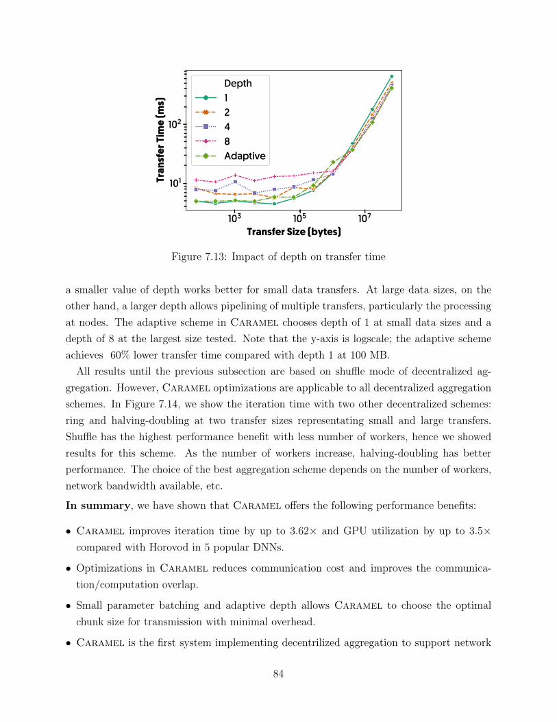
103 105 107

Transfer Size (bytes)

101

102

Tran

sfer

Tim

e (m

s)

Depth1248Adaptive

Figure 7.13: Impact of depth on transfer time

a smaller value of depth works better for small data transfers. At large data sizes, on the

other hand, a larger depth allows pipelining of multiple transfers, particularly the processing

at nodes. The adaptive scheme in Caramel chooses depth of 1 at small data sizes and a

depth of 8 at the largest size tested. Note that the y-axis is logscale; the adaptive scheme

achieves 60% lower transfer time compared with depth 1 at 100 MB.

All results until the previous subsection are based on shuffle mode of decentralized ag-

gregation. However, Caramel optimizations are applicable to all decentralized aggregation

schemes. In Figure 7.14, we show the iteration time with two other decentralized schemes:

ring and halving-doubling at two transfer sizes representating small and large transfers.

Shuffle has the highest performance benefit with less number of workers, hence we showed

results for this scheme. As the number of workers increase, halving-doubling has better

performance. The choice of the best aggregation scheme depends on the number of workers,

network bandwidth available, etc.

In summary, we have shown that Caramel offers the following performance benefits:

• Caramel improves iteration time by up to 3.62× and GPU utilization by up to 3.5×compared with Horovod in 5 popular DNNs.

• Optimizations in Caramel reduces communication cost and improves the communica-

tion/computation overlap.

• Small parameter batching and adaptive depth allows Caramel to choose the optimal

chunk size for transmission with minimal overhead.

• Caramel is the first system implementing decentrilized aggregation to support network

84

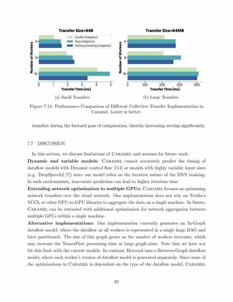
0 1 2 3 4 5Transfer Time (ms)

4

8

16Num

ber o

f Wor

kers

Transfer Size=64BShuffle (Adaptive)Ring (Adaptive)Halving Doubling (Adaptive)

(a) Small Transfers

0 100 200 300 400Transfer Time (ms)

4

8

16Num

ber o

f Wor

kers

Transfer Size=64MB

(b) Large Transfers

Figure 7.14: Performance Comparison of Different Collective Transfer Implementation inCaramel. Lower is better.

transfers during the forward pass of computation, thereby increasing overlap significantly.

7.7 DISCUSSION

In this section, we discuss limitations of Caramel and avenues for future work.

Dynamic and variable models: Caramel cannot accurately predict the timing of

dataflow models with Dynamic control flow [114] or models with highly variable input sizes

(e.g. DeepSpeech2 [7]) since our model relies on the iterative nature of the DNN training.

In such environments, inaccurate prediction can lead to higher iteration time.

Extending network optimization to multiple GPUs: Caramel focuses on optimizing

network transfers over the cloud network. Our implementation does not rely on Nvidia’s

NCCL or other GPU-to-GPU libraries to aggregate the data on a single machine. In future,

Caramel can be extended with additional optimization for network aggregation between

multiple GPUs within a single machine.

Alternative implementations: Our implementation currently generates an In-Graph

dataflow model, where the dataflow at all workers is represented in a single large DAG and

later partitioned. The size of this graph grows as the number of workers increases, which

may increase the TensorFlow processing time at large graph sizes. Note that we have not

hit this limit with the current models. In contrast, Horovod uses a Between-Graph dataflow

model, where each worker’s version of dataflow model is generated separately. Since none of

the optimizations in Caramel is dependent on the type of the dataflow model, Caramel

85

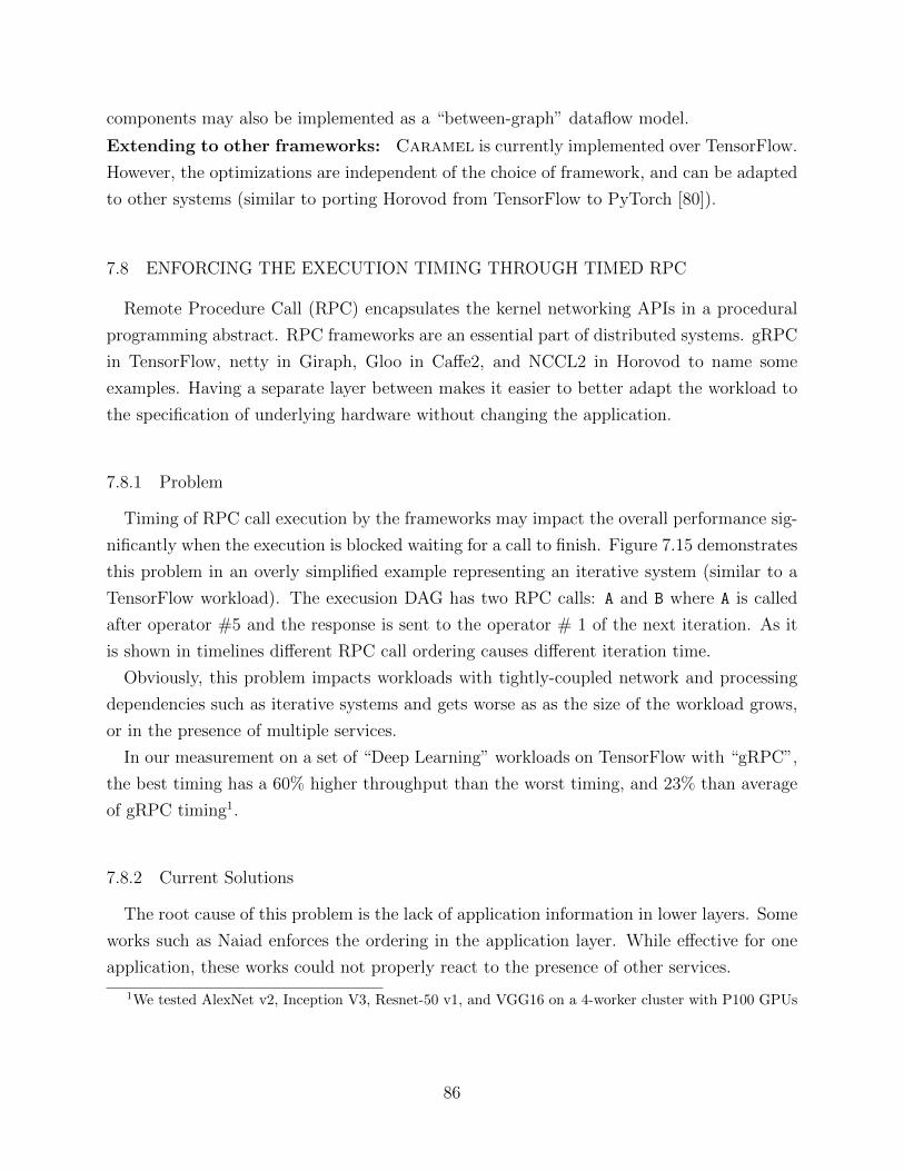
components may also be implemented as a “between-graph” dataflow model.

Extending to other frameworks: Caramel is currently implemented over TensorFlow.

However, the optimizations are independent of the choice of framework, and can be adapted

to other systems (similar to porting Horovod from TensorFlow to PyTorch [80]).

7.8 ENFORCING THE EXECUTION TIMING THROUGH TIMED RPC

Remote Procedure Call (RPC) encapsulates the kernel networking APIs in a procedural

programming abstract. RPC frameworks are an essential part of distributed systems. gRPC

in TensorFlow, netty in Giraph, Gloo in Caffe2, and NCCL2 in Horovod to name some

examples. Having a separate layer between makes it easier to better adapt the workload to

the specification of underlying hardware without changing the application.

7.8.1 Problem

Timing of RPC call execution by the frameworks may impact the overall performance sig-

nificantly when the execution is blocked waiting for a call to finish. Figure 7.15 demonstrates

this problem in an overly simplified example representing an iterative system (similar to a

TensorFlow workload). The execusion DAG has two RPC calls: A and B where A is called

after operator #5 and the response is sent to the operator # 1 of the next iteration. As it

is shown in timelines different RPC call ordering causes different iteration time.

Obviously, this problem impacts workloads with tightly-coupled network and processing

dependencies such as iterative systems and gets worse as as the size of the workload grows,

or in the presence of multiple services.

In our measurement on a set of “Deep Learning” workloads on TensorFlow with “gRPC”,

the best timing has a 60% higher throughput than the worst timing, and 23% than average

of gRPC timing1.

7.8.2 Current Solutions

The root cause of this problem is the lack of application information in lower layers. Some

works such as Naiad enforces the ordering in the application layer. While effective for one

application, these works could not properly react to the presence of other services.

1We tested AlexNet v2, Inception V3, Resnet-50 v1, and VGG16 on a 4-worker cluster with P100 GPUs

86

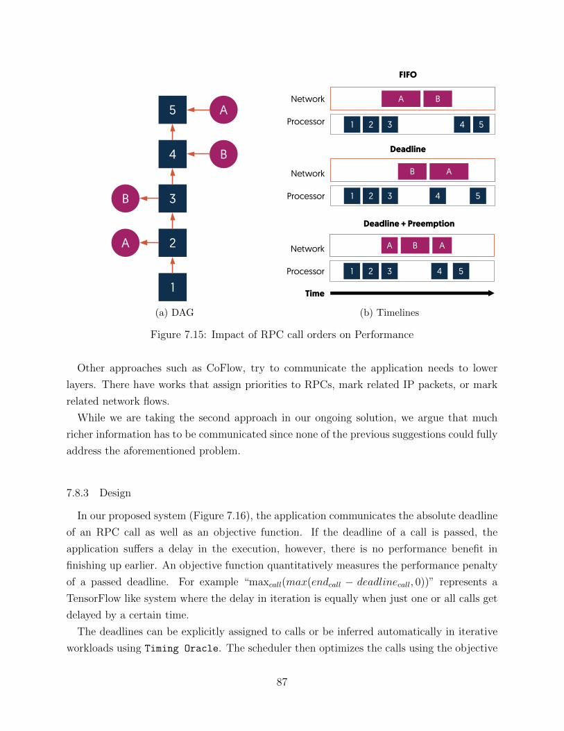
1

2

3

4

5

B

A

B

A

(a) DAG

Network

Processor

1 2 3

B

4 5

A

1 2 3

B

4 5

A

1 2 3

B

4 5

A A

Network

Processor

Network

Processor

FIFO

Deadline

Deadline + Preemption

Time

(b) Timelines

Figure 7.15: Impact of RPC call orders on Performance

Other approaches such as CoFlow, try to communicate the application needs to lower

layers. There have works that assign priorities to RPCs, mark related IP packets, or mark

related network flows.

While we are taking the second approach in our ongoing solution, we argue that much

richer information has to be communicated since none of the previous suggestions could fully

address the aforementioned problem.

7.8.3 Design

In our proposed system (Figure 7.16), the application communicates the absolute deadline

of an RPC call as well as an objective function. If the deadline of a call is passed, the

application suffers a delay in the execution, however, there is no performance benefit in

finishing up earlier. An objective function quantitatively measures the performance penalty

of a passed deadline. For example “maxcall(max(endcall − deadlinecall, 0))” represents a

TensorFlow like system where the delay in iteration is equally when just one or all calls get

delayed by a certain time.

The deadlines can be explicitly assigned to calls or be inferred automatically in iterative

workloads using Timing Oracle. The scheduler then optimizes the calls using the objective

87

Application

Timed RPC

Network

RequestRe

spon

se

Compression

Batching

Splitting

Scheduling

Reconstruction

Unbatching

Decompression

Figure 7.16: Timed RPC Architecture

function.

7.8.4 Results

We have implemented an RPC framework simulator and replaced it with gRPC in Ten-

sorFlow. In our implementation deadlines are pre-calculated from analyzing the data flow

DAG. We split the large RPC calls to make the bin packing problem in scheduling easier.

Our results show that our RPC framework achieves up to 20% higher throughput compares

to default gRPC.

7.9 RELATED WORK

Several solutions have been proposed for reducing iteration time through network accel-

eration in distributed DNN training. The first category focuses on modifying the machine

learning algorithm with the objective of optimizing network tranfers [5, 109, 116]. Caramel

does not change the DNN; it only adds additional dependencies in the dataflow DAG without

altering the underlying logic. The second class of solutions decreases network overhead by

reducing the precision of parameters [105, 27, 41]. Caramel does not change the parame-

88

ters of the DNN. The third approach is to optimize the aggregation pattern for accelerated

DNN training [37, 25, 7, 113, 4, 116]. Caramel belongs to this category.

However, prior solutions for improving communication/computation overlap [8, 29, 116]

developed for earlier layer-by-layer systems where the model is sequential cannot be adapted

to modern DAG-based systems. Caramel algorithms are not related to these prior so-

lutions. Solutions for improving communication/computation overlap in Parameter Server

(PS) based systems cannot optimize Collective communication (AR) due to significant dif-

ferences in the execution model. PS has three steps: “Push” gradients to PS, “Update”

parameters on PS, and “Pull” parameters to workers. Poseidon [116], P3 [56], and Tic-

Tac [46] overlap Pull, Update, and Push across different parameters at the same time in

PS-based aggregation. AllReduce (which Caramel tackles) has only 2 steps: “collective

reduce” of gradients followed by “Update” parameters at each worker (Fig 1). More impor-

tantly, similar techniques are used differently in Caramel and past work. E.g., Caramel

splits transfers to overlap “time on the wire” with kernel context switching and aggrega-

tion op within a single transfer. P3 splits a transfer to overlap Push and Pull of subparts.

Caramel transfers all subparts in parallel while P3 transfers sequentially.

Finally, some systems focus on increasing the communication/computation overlap. How-

ever, these solutions [8, 29, 116] were developed for earlier layer-by-layer systems where the

model is sequential. These techniques cannot be adapted to modern DAG-based systems.

Caramel algorithms are not related to these prior solutions.

Kylix [117] proposed the use of allreduce primitives (such as recursive halving-doubling

used by Caramel) in commodity clusters primarily for big data processing systems such

as Hadoop and PowerGraph. It leverages the sparsity of data to optimize network trans-

fers. While Caramel relies on the same primitives, we implement additional optimizations

tailored to the TensorFlow framework. Moreover, Caramel chooses when to do the ag-

gregation and on what data size based on the model and network characteristics. Another

work [69] that optimizes allreduce for machine learning frameworks is tailored for the HPC

environment with high speeds and not suitable for the cloud environment (InfiniBand is

54+Gbps, and Azure cloud environment provides the highest cloud bandwidth of 10Gbps.)

Horovod [90], built atop an earlier work [11], uses a decentralized aggregation pattern with

model-replica training jobs similar to Caramel. Horovod also adds communication ops to

dataflow DAG of TensorFlow. However, it redirects the communication to MPI or NCCL

allreduce implementations with limited optimizations on transfer. In contrast with Horovod,

Caramel involves significant optimization for overlap improvement and communication

cost reduction using fine-grained scheduling and batching. The large performance benefits

of Caramel over Horovod is due to these model- and network-aware optimizations.

89

ByteScheduler [82], a generic scheduler for both PS and AllReduce with network-only op-

timizations, has limitations for AllReduce workloads. It needs custom implementation for

every accelerator and network fabric. Currently, it only supports NVIDIA GPUs but not

CPU/TPU. Caramel works with all hardware supported by TensorFlow out of the box.

ByteScheduler also requires an out-of-DAG implementation of parameter optimization and

only supports SGD, Adam and RMSprop currently2. Caramel supports all TensorFlow

optimizers and auxiliary services such as checkpointing without any modification. The ran-

dom execution order of transfers, which could cause deadlock and underutilized network and

pipelining of parameters, are other problems in AllReduce that only Caramel tackles.

More importantly, prior work in this space requires changes to the underlying framework:

P3 [56] modified KVServer in MXNet, TicTac [46] modified WorkerService in TensorFlow,

ByteScheduler [82] uses out-of-DAG scheduler. Caramel works with vanilla TensorFlow

without any changes to the underlying framework.

7.10 CONCLUSION

Iteration time in distributed DNN training in cloud environment is often bottlenecked

by network transfers. In this paper, we develop Caramel to accelerate DNN training

through network transfer optimizations. Caramel identifies the appropriate aggregation

pattern for a given network environment to reduce the communication cost. The communica-

tion/computation overlap is improved with model- and network-aware optimizations. High

performance gains achieved by decentralized aggregation patterns in Caramel motivates

further research in decentralized aggregation mechanisms tailored for cloud environments.

2https://github.com/bytedance/byteps/blob/e4bbd24747470941bb5b76f542d4e8b2a9d02e1a/

example/pytorch/benchmark_bytescheduler.py#L26

90

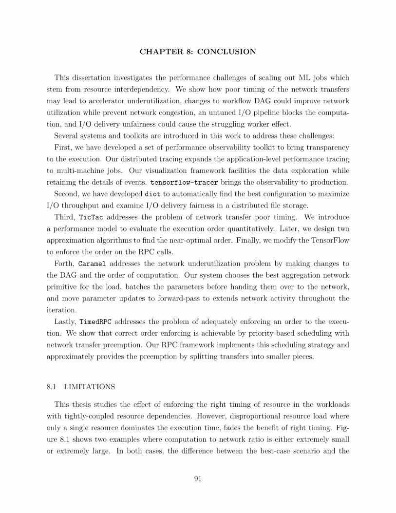
CHAPTER 8: CONCLUSION

This dissertation investigates the performance challenges of scaling out ML jobs which

stem from resource interdependency. We show how poor timing of the network transfers

may lead to accelerator underutilization, changes to workflow DAG could improve network

utilization while prevent network congestion, an untuned I/O pipeline blocks the computa-

tion, and I/O delivery unfairness could cause the struggling worker effect.

Several systems and toolkits are introduced in this work to address these challenges:

First, we have developed a set of performance observability toolkit to bring transparency

to the execution. Our distributed tracing expands the application-level performance tracing

to multi-machine jobs. Our visualization framework facilities the data exploration while

retaining the details of events. tensorflow-tracer brings the observability to production.

Second, we have developed diot to automatically find the best configuration to maximize

I/O throughput and examine I/O delivery fairness in a distributed file storage.

Third, TicTac addresses the problem of network transfer poor timing. We introduce

a performance model to evaluate the execution order quantitatively. Later, we design two

approximation algorithms to find the near-optimal order. Finally, we modify the TensorFlow

to enforce the order on the RPC calls.

Forth, Caramel addresses the network underutilization problem by making changes to

the DAG and the order of computation. Our system chooses the best aggregation network

primitive for the load, batches the parameters before handing them over to the network,

and move parameter updates to forward-pass to extends network activity throughout the

iteration.

Lastly, TimedRPC addresses the problem of adequately enforcing an order to the execu-

tion. We show that correct order enforcing is achievable by priority-based scheduling with

network transfer preemption. Our RPC framework implements this scheduling strategy and

approximately provides the preemption by splitting transfers into smaller pieces.

8.1 LIMITATIONS

This thesis studies the effect of enforcing the right timing of resource in the workloads

with tightly-coupled resource dependencies. However, disproportional resource load where

only a single resource dominates the execution time, fades the benefit of right timing. Fig-

ure 8.1 shows two examples where computation to network ratio is either extremely small

or extremely large. In both cases, the difference between the best-case scenario and the

91

0.00 0.02 0.04 0.06 0.08 0.10Communication to Computation Ratio ( )

0.0

0.2

0.4

0.6

0.8

1.0O

verla

p C

oeffi

cien

t ()

93% 95%

97%

99%

(a) Extreme Computation Load

4.00 4.25 4.50 4.75 5.00 5.25 5.50 5.75 6.00Communication to Computation Ratio ( )

16%

18%

20%

22%

(b) Extreme Network Load

Figure 8.1: Demonstration of Disproportional Resource Load

worth-case is less than 5%.

Furthermore, many of the assumptions and solutions in this dissertation presume work-

load is presented in a DAG form. However, this work needs to revisit if a more general

representation replaces DAG.

8.2 FUTURE WORKS

Explicitly timing the execution of distributed ML workload is the central idea in this

dissertation. This section discusses multiple directions to expand upon this idea:

Resources: This dissertation has explored the timing of I/O, network transfers, com-

putation, and their interplay. An organic expansion to this work is to explore other crit-

ical resources in an ML workload such as host memory, accelerator memory, caches, and

accelerator-host data bus. For example, timing can enforce the execution to reduce memory

utilization or increases cache efficiency. Moreover, a generalized solution could combine the

efficiency of multiple resources and their inter-dependency to introduce a holistic execution

executor in complex machine learning systems.

Timing Representation: DAG is an established workload representation for ML work-

loads, which clearly expresses the data and control dependencies. However, this representa-

tion leaves the runtime to choose an execution path from multiple options with very different

performance outcomes. To help the runtime to take the more performant path, in this work

we include additional data in the DAG representing the timing dependencies: TicTac used

per node priority metadata, and Caramel overloaded the control dependencies to put more

restrictions on the execution.

A research direction toward addressing this issue is a universal language to express the

timing dependencies between nodes. This language needs to be expressive enough to be able

92

to represent the complex resource inter-dependencies while keeps the runtime performance

in mind. Ultimately this universal timing language could decouple the process of finding an

optimal execution timing from the enforcing of such execution path in runtime.

Heuristics: The optimization problems in the execution timing are often NP-Hard or

harder. In this work, we used mostly empirical hand-crafted heuristics to approximate the

optimal solutions. Future researches could look at alternative approaches to solve these hard

problems. For example, with the current advancement in Deep Reinforcement Learning, it

seems ML could find approximations that are better suited for the workload in hand. Equally

important, this ML-driven approach could result in cost reduction in grid search optimization

methods such as one we used in Diot.

Workloads: This thesis mainly focuses on distributed training workloads with expensive

computation and frequent communication between steps. There are other classes of dis-

tributed ML workloads with vastly different characteristics that can benefit from execution

timing. Examples of such workloads are embarrassingly parallel jobs such as Hyperparameter

tuning or batch inferences.

93

REFERENCES

[1] Martin Abadi, Paul Barham, Jianmin Chen, Zhifeng Chen, Andy Davis, Jeffrey Dean, Matthieu Devin,Sanjay Ghemawat, Geoffrey Irving, Michael Isard, Manjunath Kudlur, Josh Levenberg, Rajat Monga,Sherry Moore, Derek G. Murray, Benoit Steiner, Paul Tucker, Vijay Vasudevan, Pete Warden, MartinWicke, Yuan Yu, and Xiaoqiang Zheng. 2016. TensorFlow: A system for large-scale machine learning.In 12th USENIX Symposium on Operating Systems Design and Implementation (OSDI 16). 265–283.

[2] Sami Abu-El-Haija, Nisarg Kothari, Joonseok Lee, Paul Natsev, George Toderici, BalakrishnanVaradarajan, and Sudheendra Vijayanarasimhan. 2016. Youtube-8m: A large-scale video classificationbenchmark. arXiv preprint arXiv:1609.08675 (2016).

[3] Akshay Agrawal, Akshay Naresh Modi, Alexandre Passos, Allen Lavoie, Ashish Agarwal, AsimShankar, Igor Ganichev, Josh Levenberg, Mingsheng Hong, Rajat Monga, and Shanqing Cai. 2019.TensorFlow Eager: A Multi-Stage, Python-Embedded DSL for Machine Learning. arXiv e-prints,Article arXiv:1903.01855 (Feb. 2019), arXiv:1903.01855 pages. arXiv:cs.PL/1903.01855

[4] Takuya Akiba, Shuji Suzuki, and Keisuke Fukuda. 2017. Extremely Large Minibatch SGD: TrainingResNet-50 on ImageNet in 15 Minutes. CoRR abs/1711.04325 (2017). arXiv:1711.04325 http:

//arxiv.org/abs/1711.04325

[5] Dan Alistarh, Demjan Grubic, Jerry Li, Ryota Tomioka, and Milan Vojnovic. 2017. QSGD:Communication-Efficient SGD via Gradient Quantization and Encoding. In Advances in Neural In-formation Processing Systems. 1707–1718.

[6] Gene M Amdahl. 1967. Validity of the single processor approach to achieving large scale computingcapabilities. In Proceedings of the April 18-20, 1967, spring joint computer conference. ACM, 483–485.

[7] Dario Amodei, Rishita Anubhai, Eric Battenberg, Carl Case, Jared Casper, Bryan Catanzaro, Jing-dong Chen, Mike Chrzanowski, Adam Coates, Greg Diamos, Erich Elsen, Jesse Engel, Linxi Fan,Christopher Fougner, Tony Han, Awni Y. Hannun, Billy Jun, Patrick LeGresley, Libby Lin, SharanNarang, Andrew Y. Ng, Sherjil Ozair, Ryan Prenger, Jonathan Raiman, Sanjeev Satheesh, David See-tapun, Shubho Sengupta, Yi Wang, Zhiqian Wang, Chong Wang, Bo Xiao, Dani Yogatama, Jun Zhan,and Zhenyao Zhu. 2015. Deep Speech 2: End-to-End Speech Recognition in English and Mandarin.CoRR abs/1512.02595 (2015). http://arxiv.org/abs/1512.02595

[8] Sebastien Arnold. 2016. An Introduction to Distributed Deep Learning. https://seba1511.com/

dist_blog/.

[9] Jens Axboe. 2019. Flexible I/O tester. Retrieved Augest (2019).

[10] Mohammad Babaeizadeh, Chelsea Finn, Dumitru Erhan, Roy Campbell, and Sergey Levine. 2018.Stochastic Variational Video Prediction. https://openreview.net/pdf?id=rk49Mg-CW

[11] Baidu Research. 2016. baidu-allreduce. https://github.com/baidu-research/baidu-allreduce.

[12] Paul Barham and Michael Isard. 2019. Machine Learning Systems Are Stuck in a Rut. In Proceedingsof the Workshop on Hot Topics in Operating Systems (HotOS ’19). ACM, New York, NY, USA,177–183. https://doi.org/10.1145/3317550.3321441

[13] Mike Barnett, Lance Shuler, Robert van De Geijn, Satya Gupta, David G Payne, and Jerrell Watts.1994. Interprocessor collective communication library (InterCom). In Scalable High-Performance Com-puting Conference, 1994., Proceedings of the. IEEE, 357–364.

94

[14] Tal Ben-Nun and Torsten Hoefler. 2018. Demystifying parallel and distributed deep learning: Anin-depth concurrency analysis. arXiv preprint arXiv:1802.09941 (2018).

[15] Leon Bottou. 2010. Large-Scale Machine Learning with Stochastic Gradient Descent. In Proceedingsof COMPSTAT’2010, Yves Lechevallier and Gilbert Saporta (Eds.). Physica-Verlag HD, Heidelberg,177–186.

[16] Leon Bottou and Olivier Bousquet. 2008. The tradeoffs of large scale learning. In Advances in neuralinformation processing systems. 161–168.

[17] Google Brain. [n. d.]. Distributed TensorFlow. https://www.tensorflow.org/deploy/distributed.

[18] Google Brain. Accessed: February 15, 2019. TensorBoard: Visualizing Learning. https://www.

tensorflow.org/guide/summaries_and_tensorboard.

[19] Peter Brucker and Sigrid Knust. 2007. Complexity results for scheduling problems.

[20] Liang-Chieh Chen, Yukun Zhu, George Papandreou, Florian Schroff, and Hartwig Adam. 2018.Encoder-decoder with atrous separable convolution for semantic image segmentation. In Proceedingsof the European conference on computer vision (ECCV). 801–818.

[21] Tianqi Chen, Mu Li, Yutian Li, Min Lin, Naiyan Wang, Minjie Wang, Tianjun Xiao, Bing Xu,Chiyuan Zhang, and Zheng Zhang. 2015. Mxnet: A flexible and efficient machine learning library forheterogeneous distributed systems. arXiv preprint arXiv:1512.01274 (2015).

[22] Tianqi Chen, Thierry Moreau, Ziheng Jiang, Haichen Shen, Eddie Q Yan, Leyuan Wang, Yuwei Hu,Luis Ceze, Carlos Guestrin, and Arvind Krishnamurthy. 2018. TVM: end-to-end optimization stackfor deep learning. arXiv preprint arXiv:1802.04799 (2018), 1–15.

[23] Yanpei Chen, Rean Griffith, Junda Liu, Randy H Katz, and Anthony D Joseph. 2009. UnderstandingTCP incast throughput collapse in datacenter networks. In Proceedings of the 1st ACM workshop onResearch on enterprise networking. ACM, 73–82.

[24] Trishul M Chilimbi, Yutaka Suzue, Johnson Apacible, and Karthik Kalyanaraman. 2014. ProjectAdam: Building an Efficient and Scalable Deep Learning Training System.. In OSDI, Vol. 14. 571–582.

[25] Minsik Cho, Ulrich Finkler, Sameer Kumar, David Kung, Vaibhav Saxena, and Dheeraj Sreedhar.2017. PowerAI DDL. arXiv preprint arXiv:1708.02188 (2017).

[26] Francois Chollet. 2015. Keras: Deep Learning for humans. https://keras.io.

[27] Matthieu Courbariaux, Yoshua Bengio, and Jean-Pierre David. 2015. Binaryconnect: Training deepneural networks with binary weights during propagations. In Advances in neural information processingsystems. 3123–3131.

[28] Henggang Cui, Alexey Tumanov, Jinliang Wei, Lianghong Xu, Wei Dai, Jesse Haber-Kucharsky,Qirong Ho, Gregory R Ganger, Phillip B Gibbons, Garth A Gibson, et al. 2014. Exploiting iterative-ness for parallel ML computations. In Proceedings of the ACM Symposium on Cloud Computing. ACM,1–14.

[29] Henggang Cui, Hao Zhang, Gregory R Ganger, Phillip B Gibbons, and Eric P Xing. 2016. GeePS:Scalable deep learning on distributed GPUs with a GPU-specialized parameter server. In Proceedingsof the Eleventh European Conference on Computer Systems. ACM, 4.

95

[30] Abdul Dakkak, Cheng Li, Abhishek Srivastava, Jinjun Xiong, and Wen-Mei Hwu. 2018. MLMod-elScope: Evaluate and Measure ML Models within AI Pipelines. arXiv preprint arXiv:1811.09737(2018).

[31] Jeffrey Dean, Greg Corrado, Rajat Monga, Kai Chen, Matthieu Devin, Mark Mao, Andrew Senior,Paul Tucker, Ke Yang, Quoc V Le, et al. 2012. Large scale distributed deep networks. In Advances inneural information processing systems. 1223–1231.

[32] Jeffrey Dean and Sanjay Ghemawat. 2004. MapReduce: Simplified Data Processing on Large Clusters.In Proceedings of the 6th Conference on Symposium on Opearting Systems Design & Implementation- Volume 6 (OSDI’04). USENIX Association, Berkeley, CA, USA, 10–10. http://dl.acm.org/

citation.cfm?id=1251254.1251264

[33] Jia Deng, Wei Dong, Richard Socher, Li-Jia Li, Kai Li, and Li Fei-Fei. 2009. Imagenet: A large-scalehierarchical image database. In 2009 IEEE conference on computer vision and pattern recognition.Ieee, 248–255.

[34] National Center for Supercomputing Applications (NCSA) at the University of Illinois. 2018. DeepLearning Major Research Instrument Project. http://www.ncsa.illinois.edu/enabling/data/

deep_learning

[35] Sanjay Ghemawat, Howard Gobioff, and Shun-Tak Leung. 2003. The Google file system. (2003).

[36] Ian Goodfellow, Yoshua Bengio, and Aaron Courville. 2016. Deep learning. MIT press.

[37] Priya Goyal, Piotr Dollar, Ross Girshick, Pieter Noordhuis, Lukasz Wesolowski, Aapo Kyrola, AndrewTulloch, Yangqing Jia, and Kaiming He. 2017. Accurate, Large Minibatch SGD: Training ImageNetin 1 Hour. arXiv preprint arXiv:1706.02677 (2017).

[38] Richard L Graham, Timothy S Woodall, and Jeffrey M Squyres. 2005. Open MPI: A flexible high per-formance MPI. In International Conference on Parallel Processing and Applied Mathematics. Springer,228–239.

[39] Brendan Gregg. 2013. Systems performance: enterprise and the cloud. Pearson Education.

[40] William Gropp, Ewing Lusk, and Anthony Skjellum. 1999. Using MPI: portable parallel programmingwith the message-passing interface. Vol. 1. MIT press.

[41] Suyog Gupta, Ankur Agrawal, Kailash Gopalakrishnan, and Pritish Narayanan. 2015. Deep learningwith limited numerical precision. In International Conference on Machine Learning. 1737–1746.

[42] Sayed Hadi Hashemi. 2018. TensorFlow Runtime Tracing Metadata Visualization. https://github.com/xldrx/tensorflow-runtime-metadata-visualization.

[43] Sayed Hadi Hashemi and Roy Campbell. 2018. Making a Case for Timed RPCs in Iterative Sys-tems. Poster Presentation in USENIX Symposium on Operating Systems Design and Implementation(OSDI).

[44] Sayed Hadi Hashemi, Sangeetha Abdu Jyothi, and Roy Campbell. 2018. Network Efficiency throughModel-Awareness in Distributed Machine Learning Systems. Poster Presentation in USENIX Sympo-sium on Networked Systems Design and Implementation (NSDI).

[45] Sayed Hadi Hashemi, Sangeetha Abdu Jyothi, and Roy Campbell. 2018. On The Importance of Exe-cution Ordering in Graph-Based Distributed Machine Learning Systems. The Conference of Systemsand Machine Learning.

96

[46] Sayed Hadi Hashemi, Sangeetha Abdu Jyothi, and Roy H Campbell. 2019. TicTac: Improving Dis-tributed Deep Learning with Communication Scheduling. The Conference of Systems and MachineLearning.

[47] Sayed Hadi Hashemi, Shadi A. Noghabi, William Gropp, and Roy H. Campbell. 2016. PerformanceModeling of Distributed Deep Neural Networks. CoRR abs/1612.00521 (2016). arXiv:1612.00521http://arxiv.org/abs/1612.00521

[48] Sayed Hadi Hashemi, Paul Rausch, Benjamin Rabe, Kuan-Yen Chou, Simeng Liu, Volodymyr Kin-dratenko, and Roy H Campbell. 2019. tensorflow-tracing: A Performance Tuning Framework forProduction. In 2019 {USENIX} Conference on Operational Machine Learning (OpML 19). 31–33.

[49] Kaiming He, Xiangyu Zhang, Shaoqing Ren, and Jian Sun. 2015. Deep Residual Learning for ImageRecognition. CoRR abs/1512.03385 (2015). arXiv:1512.03385 http://arxiv.org/abs/1512.03385

[50] Kaiming He, Xiangyu Zhang, Shaoqing Ren, and Jian Sun. 2016. Identity Mappings in Deep ResidualNetworks. CoRR abs/1603.05027 (2016). arXiv:1603.05027 http://arxiv.org/abs/1603.05027

[51] Imranul Hoque and Indranil Gupta. 2013. LFGraph: Simple and fast distributed graph analytics. InProceedings of the First ACM SIGOPS Conference on Timely Results in Operating Systems. ACM, 9.

[52] Forrest N. Iandola, Matthew W. Moskewicz, Khalid Ashraf, and Kurt Keutzer. 2016. FireCaffe: Near-Linear Acceleration of Deep Neural Network Training on Compute Clusters. In 2016 IEEE Conferenceon Computer Vision and Pattern Recognition, CVPR 2016, Las Vegas, NV, USA, June 27-30, 2016.2592–2600. https://doi.org/10.1109/CVPR.2016.284

[53] Grant Ingersoll. 2009. Introducing apache mahout. Scalable, commercialfriendly machine learning forbuilding intelligent applications. IBM (2009).

[54] Intel. 2019. PlaidML: a platform for making deep learning work everywhere. https://ai.intel.

com/plaidml

[55] Sergey Ioffe and Christian Szegedy. 2015. Batch Normalization: Accelerating Deep Network Trainingby Reducing Internal Covariate Shift. CoRR abs/1502.03167 (2015). arXiv:1502.03167 http://

arxiv.org/abs/1502.03167

[56] Anand Jayarajan, Jinliang Wei, Alexandra Fedorova, and Gennady Pekhimenko. 2019. Priority-basedParameter Propagation for Distributed DNN Training. The Conference of Systems and MachineLearning.

[57] Xianyan Jia, Shutao Song, Wei He, Yangzihao Wang, Haidong Rong, Feihu Zhou, Liqiang Xie, ZhenyuGuo, Yuanzhou Yang, Liwei Yu, et al. 2018. Highly scalable deep learning training system with mixed-precision: Training imagenet in four minutes. arXiv preprint arXiv:1807.11205 (2018).

[58] Yangqing Jia, Evan Shelhamer, Jeff Donahue, Sergey Karayev, Jonathan Long, Ross Girshick, SergioGuadarrama, and Trevor Darrell. 2014. Caffe: Convolutional architecture for fast feature embedding.In Proceedings of the 22nd ACM international conference on Multimedia. ACM, 675–678.

[59] Norman P Jouppi, Cliff Young, Nishant Patil, David Patterson, Gaurav Agrawal, Raminder Bajwa,Sarah Bates, Suresh Bhatia, Nan Boden, Al Borchers, et al. 2017. In-datacenter performance analysisof a tensor processing unit. In 2017 ACM/IEEE 44th Annual International Symposium on ComputerArchitecture (ISCA). IEEE, 1–12.

[60] Nitish Shirish Keskar, Dheevatsa Mudigere, Jorge Nocedal, Mikhail Smelyanskiy, and Ping Tak PeterTang. 2016. On large-batch training for deep learning: Generalization gap and sharp minima. arXivpreprint arXiv:1609.04836 (2016).

97

[61] Janis Keuper. 2016. Distributed Training of Deep Neuronal Networks: Theoretical and PracticalLimits of Parallel Scalability. CoRR abs/1609.06870 (2016). arXiv:1609.06870 http://arxiv.org/

abs/1609.06870

[62] Jack Kiefer, Jacob Wolfowitz, et al. 1952. Stochastic estimation of the maximum of a regressionfunction. The Annals of Mathematical Statistics 23, 3 (1952), 462–466.

[63] Alex Krizhevsky. 2014. One weird trick for parallelizing convolutional neural networks. arXiv preprintarXiv:1404.5997 (2014).

[64] Alex Krizhevsky, Ilya Sutskever, and Geoffrey E Hinton. 2012. Imagenet classification with deepconvolutional neural networks. In Advances in neural information processing systems. 1097–1105.

[65] Thorsten Kurth, Sean Treichler, Joshua Romero, Mayur Mudigonda, Nathan Luehr, Everett H.Phillips, Ankur Mahesh, Michael Matheson, Jack Deslippe, Massimiliano Fatica, Prabhat, and MichaelHouston. 2018. Exascale Deep Learning for Climate Analytics. CoRR abs/1810.01993 (2018).arXiv:1810.01993 http://arxiv.org/abs/1810.01993

[66] Chris Leary and Todd Wang. 2017. XLA: TensorFlow, compiled. TensorFlow Dev Summit (2017).

[67] Yann LeCun, Yoshua Bengio, and Geoffrey Hinton. 2015. Deep learning. nature 521, 7553 (2015),436.

[68] Mu Li, David G. Andersen, Jun Woo Park, Alexander J. Smola, Amr Ahmed, Vanja Josifovski,James Long, Eugene J. Shekita, and Bor-Yiing Su. 2014. Scaling Distributed Machine Learningwith the Parameter Server. In 11th USENIX Symposium on Operating Systems Design and Imple-mentation (OSDI 14). USENIX Association, Broomfield, CO, 583–598. https://www.usenix.org/

conference/osdi14/technical-sessions/presentation/li_mu

[69] Zhenyu Li, James Davis, and Stephen Jarvis. 2017. An Efficient Task-based All-Reduce for MachineLearning Applications. In Proceedings of the Machine Learning on HPC Environments (MLHPC’17).ACM, New York, NY, USA, Article 2, 8 pages. https://doi.org/10.1145/3146347.3146350

[70] Grzegorz Malewicz, Matthew H Austern, Aart JC Bik, James C Dehnert, Ilan Horn, Naty Leiser, andGrzegorz Czajkowski. 2010. Pregel: a system for large-scale graph processing. In Proceedings of the2010 ACM SIGMOD International Conference on Management of data. ACM, 135–146.

[71] D. Martin, C. Fowlkes, D. Tal, and J. Malik. 2001. A Database of Human Segmented Natural Imagesand its Application to Evaluating Segmentation Algorithms and Measuring Ecological Statistics. InProc. 8th Int’l Conf. Computer Vision, Vol. 2. 416–423.

[72] Xiangrui Meng, Joseph Bradley, Burak Yavuz, Evan Sparks, Shivaram Venkataraman, Davies Liu,Jeremy Freeman, DB Tsai, Manish Amde, Sean Owen, et al. 2016. Mllib: Machine learning in apachespark. The Journal of Machine Learning Research 17, 1 (2016), 1235–1241.

[73] A. Metzger, P. Leitner, D. Ivanovic, E. Schmieders, R. Franklin, M. Carro, S. Dustdar, and K. Pohl.2015. Comparing and Combining Predictive Business Process Monitoring Techniques. IEEE Trans-actions on Systems, Man, and Cybernetics: Systems 45, 2 (2015), 276–290.

[74] Azalia Mirhoseini, Anna Goldie, Hieu Pham, Benoit Steiner, Quoc V. Le, and Jeff Dean. 2018. Hier-archical Planning for Device Placement. https://openreview.net/pdf?id=Hkc-TeZ0W

[75] Azalia Mirhoseini, Hieu Pham, Quoc Le, Mohammad Norouzi, Samy Bengio, Benoit Steiner, YuefengZhou, Naveen Kumar, Rasmus Larsen, and Jeff Dean. 2017. Device Placement Optimization withReinforcement Learning. https://arxiv.org/abs/1706.04972

98

[76] Tom M Mitchell et al. 1997. Machine learning. 1997. Burr Ridge, IL: McGraw Hill 45, 37 (1997),870–877.

[77] Dan Moldovan, James Decker, Fei Wang, Andrew Johnson, Brian Lee, Zack Nado, D Sculley, TiarkRompf, and Alexander B Wiltschko. 2019. AutoGraph: Imperative-style Coding with Graph-basedPerformance. In SysML.

[78] Yuval Netzer, Tao Wang, Adam Coates, Alessandro Bissacco, Bo Wu, and Andrew Y Ng. 2011.Reading digits in natural images with unsupervised feature learning. (2011).

[79] University of Illinois at Urbana-Champaign. 2013. Illinois Campus Cluster Program. https://

campuscluster.illinois.edu

[80] Adam Paszke, Sam Gross, Soumith Chintala, and Gregory Chanan. 2017. PyTorch: Tensors anddynamic neural networks in Python with strong GPU acceleration.

[81] Adam Paszke, Sam Gross, Soumith Chintala, Gregory Chanan, Edward Yang, Zachary DeVito, ZemingLin, Alban Desmaison, Luca Antiga, and Adam Lerer. 2017. Automatic differentiation in pytorch.(2017).

[82] Yanghua Peng, Yibo Zhu, Yangrui Chen, Yixin Bao, Bairen Yi, Chang Lan, Chuan Wu, and Chuanx-iong Guo. 2019. A Generic Communication Scheduler for Distributed DNN Training Acceleration. InProceedings of the 27th ACM Symposium on Operating Systems Principles (SOSP ’19). Association forComputing Machinery, New York, NY, USA, 16–29. https://doi.org/10.1145/3341301.3359642

[83] Michael L. Pinedo. 2008. Scheduling: Theory, Algorithms, and Systems (3rd ed.). Springer PublishingCompany, Incorporated.

[84] Bryan A Plummer, Liwei Wang, Chris M Cervantes, Juan C Caicedo, Julia Hockenmaier, and SvetlanaLazebnik. 2015. Flickr30k entities: Collecting region-to-phrase correspondences for richer image-to-sentence models. In Proceedings of the IEEE international conference on computer vision. 2641–2649.

[85] Herbert Robbins and Sutton Monro. 1951. A stochastic approximation method. The annals of math-ematical statistics (1951), 400–407.

[86] David E Rumelhart, Geoffrey E Hinton, Ronald J Williams, et al. 1988. Learning representations byback-propagating errors. Cognitive modeling 5, 3 (1988), 1.

[87] Frank B Schmuck and Roger L Haskin. 2002. GPFS: A Shared-Disk File System for Large ComputingClusters.. In FAST, Vol. 2.

[88] Philip Schwan et al. 2003. Lustre: Building a file system for 1000-node clusters. In Proceedings of the2003 Linux symposium, Vol. 2003. 380–386.

[89] Frank Seide and Amit Agarwal. 2016. CNTK: Microsoft’s open-source deep-learning toolkit. In Pro-ceedings of the 22nd ACM SIGKDD International Conference on Knowledge Discovery and DataMining. ACM, 2135–2135.

[90] Alexander Sergeev and Mike Del Balso. 2018. Horovod: fast and easy distributed deep learning inTensorFlow. CoRR abs/1802.05799 (2018). arXiv:1802.05799 http://arxiv.org/abs/1802.05799

[91] Spencer Shepler, Mike Eisler, David Robinson, Brent Callaghan, Robert Thurlow, David Noveck, andCarl Beame. 2003. Network file system (NFS) version 4 protocol. Network (2003).

[92] Ben Shneiderman. 2003. The eyes have it: A task by data type taxonomy for information visualizations.In The craft of information visualization. Elsevier, 364–371.

99

[93] Konstantin Shvachko, Hairong Kuang, Sanjay Radia, Robert Chansler, et al. 2010. The hadoopdistributed file system.. In MSST, Vol. 10. 1–10.

[94] Svetlana Sicular and Kenneth Brant. 2018. Hype Cycle for Artificial Intelligence, 2018. (July 2018).

[95] Karen Simonyan and Andrew Zisserman. 2014. Very deep convolutional networks for large-scale imagerecognition. arXiv preprint arXiv:1409.1556 (2014).

[96] Srinivas Sridharan, Karthikeyan Vaidyanathan, Dhiraj Kalamkar, Dipankar Das, Mikhail E Smorkalov,Mikhail Shiryaev, Dheevatsa Mudigere, Naveen Mellempudi, Sasikanth Avancha, Bharat Kaul, et al.2018. On Scale-out Deep Learning Training for Cloud and HPC. arXiv preprint arXiv:1801.08030(2018).

[97] Christian Szegedy, Wei Liu, Yangqing Jia, Pierre Sermanet, Scott E. Reed, Dragomir Anguelov, Du-mitru Erhan, Vincent Vanhoucke, and Andrew Rabinovich. 2014. Going Deeper with Convolutions.CoRR abs/1409.4842 (2014). arXiv:1409.4842 http://arxiv.org/abs/1409.4842

[98] Christian Szegedy, Vincent Vanhoucke, Sergey Ioffe, Jonathon Shlens, and Zbigniew Wojna.2015. Rethinking the Inception Architecture for Computer Vision. CoRR abs/1512.00567 (2015).arXiv:1512.00567 http://arxiv.org/abs/1512.00567

[99] Christian Szegedy, Vincent Vanhoucke, Sergey Ioffe, Jon Shlens, and Zbigniew Wojna. 2016. Rethink-ing the inception architecture for computer vision. In Proceedings of the IEEE conference on computervision and pattern recognition. 2818–2826.

[100] Bokeh Development Team. 2014. Bokeh: Python library for interactive visualization. (2014).

[101] TensorFlow. 2019. tf.distribute.experimental.MultiWorkerMirroredStrategy.https://www.tensorflow.org/api_docs/python/tf/distribute/experimental/

MultiWorkerMirroredStrategy. (Accessed on 09/09/2019).

[102] Rajeev Thakur and William D Gropp. 2003. Improving the performance of collective operationsin MPICH. In European Parallel Virtual Machine/Message Passing Interface Users’ Group Meeting.Springer, 257–267.

[103] Philippe Tillet, HT Kung, and David Cox. 2019. Triton: an intermediate language and compiler fortiled neural network computations. In Proceedings of the 3rd ACM SIGPLAN International Workshopon Machine Learning and Programming Languages. ACM, 10–19.

[104] Seiya Tokui, Kenta Oono, Shohei Hido, and Justin Clayton. 2015. Chainer: a next-generation opensource framework for deep learning. In Proceedings of workshop on machine learning systems (Learn-ingSys) in the twenty-ninth annual conference on neural information processing systems (NIPS), Vol. 5.1–6.

[105] Vincent Vanhoucke, Andrew Senior, and Mark Z Mao. 2011. Improving the speed of neural networkson CPUs. In Proc. Deep Learning and Unsupervised Feature Learning NIPS Workshop, Vol. 1. Citeseer,4.

[106] Ashish Vaswani, Samy Bengio, Eugene Brevdo, Francois Chollet, Aidan N Gomez, Stephan Gouws,Llion Jones, Lukasz Kaiser, Nal Kalchbrenner, Niki Parmar, et al. 2018. Tensor2tensor for neuralmachine translation. arXiv preprint arXiv:1803.07416 (2018).

[107] Vinod Kumar Vavilapalli, Arun C Murthy, Chris Douglas, Sharad Agarwal, Mahadev Konar, RobertEvans, Thomas Graves, Jason Lowe, Hitesh Shah, Siddharth Seth, et al. 2013. Apache hadoop yarn:Yet another resource negotiator. In Proceedings of the 4th annual Symposium on Cloud Computing.ACM, 5.

100

[108] Abhishek Verma, Luis Pedrosa, Madhukar Korupolu, David Oppenheimer, Eric Tune, and JohnWilkes. 2015. Large-scale cluster management at Google with Borg. In Proceedings of the TenthEuropean Conference on Computer Systems. ACM, 18.

[109] Wei Wen, Cong Xu, Feng Yan, Chunpeng Wu, Yandan Wang, Yiran Chen, and Hai Li. 2017. Tern-grad: Ternary gradients to reduce communication in distributed deep learning. In Advances in NeuralInformation Processing Systems. 1508–1518.

[110] Reynold S Xin, Joseph E Gonzalez, Michael J Franklin, and Ion Stoica. 2013. Graphx: A resilientdistributed graph system on spark. In First International Workshop on Graph Data ManagementExperiences and Systems. ACM, 2.

[111] Arvind Thiagarajan Yi Zhuang and Tim Sweeney. 2019. Ranking Tweets with TensorFlow. https:

//medium.com/tensorflow/ranking-tweets-with-tensorflow-932d449b7c4

[112] Yang You, Igor Gitman, and Boris Ginsburg. 2017. Scaling sgd batch size to 32k for imagenet training.arXiv preprint arXiv:1708.03888 6 (2017).

[113] Yang You, Zhao Zhang, Cho-Jui Hsieh, and James Demmel. 2017. 100-epoch ImageNet Training withAlexNet in 24 Minutes. CoRR abs/1709.05011 (2017). arXiv:1709.05011 http://arxiv.org/abs/

1709.05011

[114] Yuan Yu, Martın Abadi, Paul Barham, Eugene Brevdo, Mike Burrows, Andy Davis, Jeff Dean, SanjayGhemawat, Tim Harley, Peter Hawkins, Michael Isard, Manjunath Kudlur, Rajat Monga, DerekMurray, and Xiaoqiang Zheng. 2018. Dynamic Control Flow in Large-scale Machine Learning. InProceedings of the Thirteenth EuroSys Conference (EuroSys ’18). ACM, New York, NY, USA, Article18, 15 pages. https://doi.org/10.1145/3190508.3190551

[115] Matei Zaharia, Mosharaf Chowdhury, Michael J Franklin, Scott Shenker, and Ion Stoica. 2010. Spark:Cluster computing with working sets. HotCloud 10, 10-10 (2010), 95.

[116] Hao Zhang, Zeyu Zheng, Shizhen Xu, Wei Dai, Qirong Ho, Xiaodan Liang, Zhiting Hu, JinliangWei, Pengtao Xie, and Eric P. Xing. 2017. Poseidon: An Efficient Communication Architecture forDistributed Deep Learning on GPU Clusters. In 2017 USENIX Annual Technical Conference (USENIXATC 17). USENIX Association, Santa Clara, CA, 181–193. https://www.usenix.org/conference/

atc17/technical-sessions/presentation/zhang

[117] H. Zhao and J. Canny. 2014. Kylix: A Sparse Allreduce for Commodity Clusters. In 43rd InternationalConference on Parallel Processing. 273–282. https://doi.org/10.1109/ICPP.2014.36

101